Where do all the Supercurvature Modes Go?

Abstract

In the hyperbolic slicing of de Sitter space appropriate for open universe models, a curvature scale is present and supercurvature fluctuations are possible. In some cases, the expansion of a scalar field in the Bunch-Davies vacuum includes supercurvature modes, as shown by Sasaki, Tanaka and Yamamoto. We express the normalizable vacuum supercurvature modes for a massless scalar field in terms of the basis modes for the spatially-flat slicing of de Sitter space.

I Introduction

Scalar fields in de Sitter spacetime have long provided a testing ground for issues of quantum field theory in curved spacetime [1, 2]. Further motivation for their study stems from the central role they play in inflationary cosmology [3]. Several different coordinate systems can be used to cover de Sitter space, and subtleties in the quantization of fields can arise in some of the less familiar coordinate systems. These subtleties have been highlighted by recent models of open inflation [4, 5], in which two periods of inflation are separated by nucleation of a bubble. The bubble interior includes an open universe ($\Omega_{0}<1$), where we could be living today, described by hyperbolic, spatially-curved coordinates [6].

A key difference between these hyperbolic coordinates and the more familiar spatially-flat slicing of de Sitter space is the presence of a curvature scale. This in turn leads to the possibility of supercurvature [7] fluctuations, fluctuations with wavelength longer than the curvature scale. Unlike the continuum of modes familiar from the spatially-flat slicing of de Sitter space, a normalizable supercurvature mode may exist for an isolated, discrete eigenvalue of the spatial Laplacian, or not at all. Although such modes have no analogue in the spatially-flat slicing of de Sitter space, it has been shown [8] (see also [9]) that the supercurvature modes must be included in the vacuum spectra of low-mass scalar fields in order to produce a complete set of states, and hence the proper Wightman function.

For massless, minimally-coupled scalar fields in de Sitter space, there is in addition a well-known infrared divergence in the (coordinate-independent) Wightman function. The infrared divergence is related to a dynamical zero mode in the spectrum of a massless field [10, 11]. Kirsten and Garriga [11] covariantly quantized this zero mode in a spatially-closed slicing of de Sitter space. Extending their result from these closed coordinates to the coordinate system appropriate to open inflation has not yet been done. Here we identify the zero mode as one of the supercurvature modes when quantizing the minimally-coupled massless field in the open hyperbolic coordinates.

It has already been noted that supercurvature modes can make significant contributions to the fluctuations in the cosmic microwave background (CMB) radiation, and several of their effects have been calculated for models of open inflation [12, 13, 14, 15]. (The massless field zero-mode subtleties, except for a variant studied in [15], do not arise for these specific CMB calculations, which are sensitive to higher multipoles.) In addition to contributing to observable density fluctuations, such long wavelength, supercurvature modes might play a role [16] at the end of inflation, when recent advances [17] in the theory of reheating are taken into consideration.

In summary, increased understanding of these supercurvature modes is motivated both by general questions of quantizing fields in curved backgrounds, and by recent inflationary model-building. We will focus here on the example of supercurvature modes for a massless, minimally-coupled scalar field, expressing them as a sum over the basis modes for a spatially-flat slicing of de Sitter space. This overlap gives a measure of “where all the supercurvature modes go” in the familiar flat-space spectrum of such fields. The massless case is chosen for tractability, and questions about the zero mode are postponed for future work [18].

Throughout this paper, we consider only an unperturbed de Sitter metric; a more complete treatment would include study of the backreaction of such fields on the background metric. Because the supercurvature modes stretch beyond the horizon, any such study of the coupled metric fluctuations would need to pay special attention to the gauge subtleties which always accompany superhorizon fluctuations [19], and such issues are not pursued here.

In section II, the two covers of de Sitter space (including the flat and hyperbolic slicings) are given, and the field quantization pertinent to open inflation in both systems is reviewed. As these supercurvature modes have no analogue in the usual flat slicing of de Sitter space, this section gathers some previous work on supercurvature modes and provides notation and context for the rest of the paper. Section III specializes to the massless case. The explicit calculation of the overlap for some of these supercurvature modes and the more familiar flat space modes is given, and indicates a general form for the overlap between all the massless supercurvature and spatially flat modes. We verify this general form by integrating over the spatially flat modes, weighted by the overlap, to obtain the original supercurvature modes. Concluding remarks follow in Section IV. Three Appendices include the supercurvature mode normalization at fixed time in the flat coordinates, and details of the overlap calculation along different hypersurfaces within de Sitter space.

II De Sitter Spacetime and Scalar Field Quantization

We begin by considering de Sitter spacetime as embedded within a 5-dimensional Minkowski spacetime, with the five coordinates subject to the constraint [1]:

$$-\left(z^{0}\right)^{2}+\sum_{i=1}^{4}\left(z^{i}\right)^{2}=1.$$ (1)

The radius of the embedded spacetime, $H^{-1}$, is scaled to unity.

A spatially flat slicing (see, e.g. [1]) which partially covers the resulting 4-dimensional de Sitter spacetime is

$$z^{0} = \sinh t_{f}+\frac{1}{2}e^{t_{f}}r_{f}^{2}=-\frac{1}{2\eta}\left(1+r_{f}^{2}\right)+\frac{1}{2}\eta,$$ (2)

$$z^{4} = \cosh t_{f}-\frac{1}{2}e^{t_{f}}r_{f}^{2}=-\frac{1}{2\eta}\left(1-r_{f}^{2}\right)-\frac{1}{2}\eta,$$ (3)

$$\vec{z} = e^{t_{f}}r_{f}\vec{\Omega}=-\frac{r_{f}}{\eta}\vec{\Omega},$$ (4)

where $\vec{\Omega}\equiv(\sin\theta\cos\varphi,\>\sin\theta\sin\varphi,\>\cos\theta)$, and conformal time $d\eta=a^{-1}dt_{f}$, or $\eta=-a^{-1}(t_{f})=-e^{-t_{f}}$. Here $r_{f}\geq 0$, $-\infty<\eta\leq 0$. (See Figure 1.)

FIG. 1.: De Sitter spacetime as covered by the coordinates in equation (4). Solid lines are lines of constant $r$, and dashed lines are lines of constant $\eta$.

The metric on this portion of the spacetime is

$$ds_{f}^{2}=\eta^{-2}\left[-d\eta^{2}+dr_{f}^{2}+r_{f}^{2}d\Omega^{2}\right],$$ (5)

where $d\Omega^{2}\equiv d\theta^{2}+\sin^{2}\theta d\varphi^{2}$. The coordinates $x_{f}$ and metric $ds_{f}^{2}$ are useful in ordinary models of inflation, in which the spatial curvature quickly becomes completely negligible. These coordinates $x_{f}$ cover only that half of the total spacetime with $z^{0}+z^{4}\geq 0$. Replacing $z^{4}\to-z^{4}$ in the above produces a second flat coordinate system.

In contrast, for models of open inflation, open hyperbolic coordinates are appropriate inside the open universe. This coordinate patch is part of the full de Sitter spacetime (discussed in detail by [8, 20]) as shown in Figure 2.

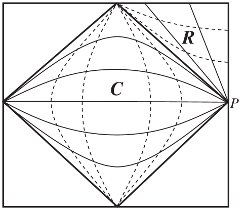
FIG. 2.: De Sitter spacetime as covered by the coordinates in equation (8). Solid lines are lines of constant $r$, and dashed lines are lines of constant $t$. If a (thin-walled) bubble nucleated with center at point $P$, then region $R$, the forward light cone of point $P$, would contain in the interior of the nucleated bubble. In models of open inflation, region $R$ would contain our observable universe at some time $t$ inside the light cone corresponding to $t=0$.

The two most important of these regions for our purposes here are region $C$, a large, compact subspace, and region $R$, an open hyperboloid bordering region $C$. These are related to the embedding coordinates by

$$\;z^{0} = \cos t_{c}\sinh r_{c}=\sinh t_{r}\cosh r_{r},$$ (6)

$$\;z^{4} = \sin t_{c}=\cosh t_{r},$$ (7)

$$\vec{z}\; = \cos t_{c}\cosh r_{c}\vec{\Omega}=\sinh t_{r}\sinh r_{r}\vec{\Omega}.$$ (8)

These coordinates lie in the ranges

$$-\frac{\pi}{2}\leq t_{c}\leq\frac{\pi}{2}\>\>,\>\>-\infty<r_{c}<\infty\>\>{\rm and}\;\>\>0\leq t_{r}\>\>,\>\>0\leq r_{r},$$ (9)

and are related by the analytic continuation $t_{r}=it_{c}-{i\pi\over 2}$ and $r_{r}=r_{c}+{i\pi\over 2}$. The corresponding metrics are

$$ds_{c}^{2} = dt_{c}^{2}+\cos^{2}t_{c}\left[-dr_{c}^{2}+\cosh^{2}r_{c}d\Omega^{2}\right],$$ (10)

$$ds_{r}^{2} = -dt_{r}^{2}+\sinh^{2}t_{r}\left[dr_{r}^{2}+\sinh^{2}r_{r}d\Omega^{2}\right].$$ (11)

Note that $r_{c}$ plays the role of ‘time’ within region $C$.

The forward light cone of the point $P$ in Figure 2 is the center of the nucleated bubble in models of open inflation, so that region $R$ contains the spatially-open universe we may be in today. Region $C$ is of interest because surfaces of fixed time, $r_{c}={\rm constant}$, correspond to Cauchy surfaces for de Sitter space. Quantizing on a Cauchy surface in $C$ thus specifies all of the “initial data” for the system, including the initial conditions for the spatially-open universe inside region $R$.

The equation of motion for a scalar field of mass $M$ in this space is

$$\left(\Box-M^{2}\right)\phi(x)=\left((\sqrt{-g})^{-1}\partial_{\mu}\left[(\sqrt{-g})g^{\mu\nu}\partial_{\nu}\right]-M^{2}\right)\phi(x)=0,$$ (12)

and separation of variables gives a family of solutions $\phi_{k\ell m}(x)$. To quantize, $\phi$ and its canonically conjugate momentum $\Pi$ are promoted to Heisenberg operators, and expanded as

$$\hat{\phi}(x)=\sum_{k\ell m}\left[\phi_{k\ell m}(x)\hat{a}_{k\ell m}+\overline{\phi}_{k\ell m}(x)\hat{a}^{\dagger}_{k\ell m}\right]$$ (13)

and similarly for $\hat{\Pi}$. The creation and annihilation operators satisfy $[\hat{a}_{k\ell m},\>\hat{a}^{\dagger}_{k^{\prime}\ell^{\prime}m^{\prime}}]=\delta(k-k^{\prime})\delta_{\ell^{\prime}\ell}\delta_{m^{\prime}m}$ with the other commutators vanishing. Here an overline denotes complex conjugation, $\sum_{k\ell m}$ is a placeholder for the appropriate measure, and the choice of vacuum state satisfying $\hat{a}_{k\ell m}|0\rangle=0$ for all $(k,\ell,m)$ provides a division into positive and negative frequency modes. The fixed-time canonical commutation relations, $[\hat{\phi}(x),\hat{\Pi}(x^{\prime})]=i\delta^{3}(\vec{x}-\vec{x}^{\prime})$ then imply that

$$(\phi_{k\ell m},\>\phi_{k^{\prime}\ell^{\prime}m^{\prime}}) = \delta\left(k-k^{\prime}\right)\delta_{\ell^{\prime}\ell}\delta_{m^{\prime}m}\>\>,\>\>(\phi_{k\ell m},\>\overline{\phi}_{k^{\prime}\ell^{\prime}m^{\prime}})=0\>\>,$$ (14)

$$(\overline{\phi}_{k\ell m},\>\overline{\phi}_{k^{\prime}\ell^{\prime}m^{\prime}}) = -\delta\left(k-k^{\prime}\right)\delta_{\ell^{\prime}\ell}\delta_{m^{\prime}m},$$ (15)

where the Klein-Gordon inner product is defined by

$$(\phi_{k\ell m},\>\phi_{k^{\prime}\ell^{\prime}m^{\prime}})\equiv-\int_{\Sigma}\left(\phi_{k\ell m}\>{\mathop{\partial_{\mu}}\limits^{\leftrightarrow}}\>\overline{\phi}_{k^{\prime}\ell^{\prime}m^{\prime}}\right)\sqrt{-g_{\Sigma}}\>n^{\mu}\>d\Sigma\;.$$ (16)

Here $\Sigma$ is a (spacelike) Cauchy surface and $n^{\mu}$ is a future-directed unit vector normal to this surface. (The extra factor of $i$ which multiplies the righthand side of equation (16) in [1] is absent here because of our different sign convention for the metric.) This inner product is independent of Cauchy surface, and more generally is independent of the choice of $\Sigma$, as long as the fields fall off sufficiently quickly on the time-like boundaries.

The physically-motivated choice of initial vacuum state in models of inflation is the Bunch-Davies vacuum [22], which respects the symmetries of de Sitter space and reduces to the Minkowski space vacuum at early times and over short distances. For the flat slicing, the Bunch-Davies positive-frequency modes are

$$\phi_{k\ell m}(x_{f})=\frac{k}{\sqrt{2}}\exp\left[i\frac{\pi}{2}\left(\nu+\frac{1}{2}\right)\right]\frac{(-\eta)^{1/2}}{a(\eta)}H_{\nu}^{(1)}(-k\eta)j_{\ell}(kr_{f})Y_{\ell m}(\Omega),$$ (17)

where $\nu\equiv\sqrt{{9\over 4}-M^{2}}$, $H_{\nu}^{(1)}(z)$ is a Hankel function of the first kind, $j_{\ell}(z)$ is a spherical Bessel function, and $Y_{\ell m}(\Omega)$ is the usual spherical harmonic. The measure in equation (13) for the expansion in flat modes $\phi_{k\ell m}$ is $\sum_{k\ell m}=\int_{0}^{\infty}dk\sum_{\ell=0}^{\infty}\sum_{m=-\ell}^{\ell}$.

For the hyperbolic slicing with the metric $ds_{c}^{2}$ of equation (11), the positive-frequency solutions to the equations of motion are [4, 8, 23]

$$u_{p\ell m}(x)=\frac{\chi_{p}(t_{c})}{a(t_{c})}f_{pl}(r_{c})Y_{\ell m}(\Omega),$$ (18)

where

$$\chi_{p}(t_{c}) = \alpha_{p}(\nu^{\prime})P^{-ip}_{\nu^{\prime}}(\sin t_{c})+\beta_{p}(\nu^{\prime})P^{ip}_{\nu^{\prime}}(\sin t_{c})\;,$$ (19)

$$f_{p\ell}(r_{c}) = \frac{P^{-\ell-1/2}_{ip-1/2}(i\sinh r_{c})}{\sqrt{i\cosh r_{c}}},$$ (20)

and

$$\nu^{\prime}\equiv\nu-{1\over 2}=\sqrt{{9\over 4}-M^{2}}-{1\over 2}\;.$$ (21)

Here $P^{\mu}_{\nu}(z)$ is an associated Legendre function of the first kind, while the specific forms of $\alpha_{p},\beta_{p}$ will not be needed. Within region $C$, the $f_{p\ell}(r_{c})$ play the role of positive-frequency solutions, and the $\chi_{p}(t_{c})$ are spatial eigenfunctions; when continued into region $R$, these roles are reversed.

A Friedmann-Robertson-Walker metric with spatial curvature $K$ and cosmic scale factor $a(t)$ has a physical curvature length scale $a(t)/|K|$. For a flat universe the comoving curvature length scale thus runs off to infinity, whereas in a spatially closed or open metric, the comoving curvature length scale is $+1$. Eigenvalues of the (region $R$) spatial Laplacian in this background are $-(k/a)^{2}$, where $(k/a)$ is the inverse of a physical length: $k/a=1/x_{\rm phys}$, with $0\leq k^{2}<\infty$. Defining $p^{2}\equiv k^{2}-1$, $p^{2}>0$ for subcurvature modes, and $-1<p^{2}\leq 0$ for supercurvature modes. The continuum of subcurvature modes $0\leq p\leq\infty$ is sufficient to describe a Gaussian random field in region $R$, see [7] for detailed discussion. In addition, for $p^{2}<0$, inner products of the form (16) on fixed-time (non-Cauchy) surfaces within region $R$ diverge, and so all supercurvature modes naively appear to be unnormalizable. Studying quantization and completeness more appropriately on a fixed time $r_{c}$ Cauchy surface in region $C$, it was found in [8] that for $M^{2}<2H^{2}$ (restoring the Hubble radius, $H^{-1}$), supercurvature modes are normalizable in vacuum for a discrete value of $p$. In addition, it was shown there that this value of $p$ must be included to obtain the correct Wightman function for the Bunch-Davies vacuum. (See also [9].)

This discrete normalizable supercurvature mode can be understood as follows [8, 23]. Its presence is suggested by an analogy between these supercurvature modes and bound states in a potential. The only dependence on $M$ in the wavefunctions is in the ‘spatial’ (in region $C$) eigenfunctions $\chi_{p}(t_{c})$. Defining $\sin t_{c}\equiv\tanh u$, the equation of motion for $\chi_{p}$ becomes

$$\left[-\frac{d^{2}}{du^{2}}+U(u)\right]\chi_{p} = p^{2}\chi_{p}\;,$$ (22)

$$U(u) \equiv \frac{M^{2}-2}{\cosh^{2}u}.$$ (23)

This is a one-dimensional Schrödinger-like equation with the potential $U(u)$ and energy $p^{2}$. As noted in [13, 14, 23], the potential $U(u)$ vanishes as $u\rightarrow\pm\infty$, revealing that in this limit there exists a continuous spectrum of modes with $p^{2}\geq 0$. But over finite intervals of $u$, if the mass of the field satisfies $M^{2}<2$, the potential $U(u)$ has a valley and the modes $\chi_{p}$ behave as discrete bound states with $p^{2}<0$. As DeWitt has shown, such discrete states in a field’s spectrum are generic for fields quantized on compact subspaces. [24]

The inner product on this space is proportional to

$$\int_{-\infty}^{\infty}du\>\chi_{p}(\tanh u)\overline{\chi}_{p^{\prime}}(\tanh u)\;,$$ (24)

so for normalizability, $\chi_{p}(\tanh u)$ must be bounded as $u\to\pm\infty$. (A similar argument is found in the appendix of [8].) A supercurvature mode has $p^{2}<0$ and $p^{2}+1\geq 0$, so define $p=i\Lambda$, with $0\leq\Lambda\leq 1$, and $\Lambda$ real. The asymptotics of $\chi_{p}$ near $\tanh u\rightarrow\pm 1$ yields (cf. [23]):

$$\Gamma(1\mp ip)P^{\pm ip}_{\nu^{\prime}}(\tanh u)\sim e^{\pm ipu}\>\>,\>\>u\rightarrow\infty.$$ (25)

This is finite only for $P^{+ip}_{\nu^{\prime}}$ since $ip=-\Lambda<0$, thus $\beta_{p}=0$ for the supercurvature modes. The limit of $P^{ip}_{\nu^{\prime}}(\tanh u)$ as $u\to-\infty$ is [23]

$$\Gamma(1+\Lambda)P^{-\Lambda}_{\nu^{\prime}}(\tanh u)\sim\frac{\Gamma(1+\Lambda)\Gamma(\Lambda)}{\Gamma(1+{\nu^{\prime}}+\Lambda)\Gamma(\Lambda-{\nu^{\prime}})}e^{\Lambda|u|}+\frac{\Gamma(1+\Lambda)\Gamma(-\Lambda)}{\Gamma(-{\nu^{\prime}})\Gamma(1+{\nu^{\prime}})}e^{-\Lambda|u|}\>,\>u\rightarrow-\infty.$$ (26)

As $0<\Lambda\leq 1$ is non-negative and $0\leq{\rm Re}\;{\nu^{\prime}}\leq 1$, the coefficient of $e^{\Lambda|u|}$ vanishes only if $\Lambda={\nu^{\prime}}$, producing an isolated value of $p$ which is normalizable. (Note that for subcurvature modes, with $p$ real and non-negative, the solution $\chi_{p}(t_{c})$ simply oscillates at both endpoints and so remains finite.)

The Klein Gordon normalized supercurvature modes are then

$$u_{\Lambda\ell m}(x_{c}) = N_{\Lambda\ell m}(-i\cos t_{c})^{{\nu^{\prime}}-1}\frac{P^{-\ell-1/2}_{-\Lambda-1/2}(i\sinh r_{c})}{\sqrt{i\cosh r_{c}}}Y_{\ell m}(\Omega),$$ (27)

$$N_{\Lambda\ell m} \equiv \left[\frac{\Gamma({\nu^{\prime}}+1/2)\Gamma(-{\nu^{\prime}}+\ell+1)\Gamma({\nu^{\prime}}+\ell+1)}{2\sqrt{\pi}\Gamma({\nu^{\prime}})}\right]^{1/2}\;.$$ (28)

The scalar field in region $C$ is expanded as [8]

$$\hat{\phi}(x_{c}) = \int_{0}^{\infty}dp\sum_{\ell,m}\left[u_{p\ell m}(x_{c})\hat{a}_{p\ell m}+{\rm H.c.}\right]+\sum_{\ell,m}\left[u_{\Lambda\ell m}(x_{c})\hat{a}_{\Lambda\ell m}+{\rm H.c.}\right]$$ (29)

$$\equiv \hat{\phi}_{(p)}(x_{c})+\hat{\phi}_{(\Lambda)}(x_{c}),$$ (30)

where “H.c” denotes the Hermitian conjugate, and $\sum_{\ell,m}\equiv\sum_{\ell=0}^{\infty}\sum_{m=-\ell}^{\ell}$. Once quantized, these modes may be continued into region $R$. In the presence of a bubble wall [14], rather than in the vacuum, the value of $\Lambda$ may change and a supercurvature mode may appear even for $M^{2}>2$, depending on the details of the model. The normalizability conditions may be solved for numerically. In the absence of gravity, there is also a supercurvature mode for the fluctuations of the bubble wall itself, which appears to become singular once gravity is included [26].

III Overlap of Supercurvature with Flat Modes for a Massless Field

We now re-express these supercurvature modes $u_{\Lambda=1\,\ell m}$ in terms of the spatially-flat modes $\phi_{k\ell m}$ for a massless scalar field. There are two things to consider, however, before proceeding to the calculation. First, for $M=0$, the $\ell=0$ supercurvature mode of equation (28) is constant. Consequently its Klein-Gordon inner product is zero and its norm (proportional to the square root of the inverse of this norm) diverges as $\Gamma^{1/2}(\ell=0)$. Including this state naively in the Wightman function sum over states will thus diverge as well. It is known that the Wightman function for a massless, minimally-coupled scalar field in de Sitter spacetime is infrared divergent [10, 11], and in this particular slicing, the specific state $u_{\Lambda=1,00}$ appears to be the lone source of the divergence.
The $r_{c}$-dependent portion of the equations of motion in region $C$, are exactly like a $(2,1)$-dimensional spacetime with scale factor $a(r_{c})=\cosh r_{c}$, For positive frequency modes,

$$\left[\frac{1}{a^{2}(r_{c})}\frac{\partial}{\partial r_{c}}\left(a^{2}(r_{c})\frac{\partial}{\partial r_{c}}\right)+\left(1+p^{2}\right)+\frac{\ell(\ell+1)}{a^{2}(r_{c})}\right]\{f_{pl}(r_{c})Y_{\ell m}(\Omega)\}=0\;$$ (31)

and the ‘frequency’ $\omega_{r_{c}}$ associated with the time-coordinate may then be written

$$\omega_{r_{c}}^{2}=(1+p^{2})+\frac{\ell(\ell+1)}{a^{2}(r_{c})},$$ (32)

the analogue of $\omega^{2}=M^{2}+k^{2}/a^{2}(t)$. This $\omega_{r_{c}}$ vanishes only for $p=i$ and $\ell=0$, indicating a zero mode corresponding to the symmetry $\phi\rightarrow\phi+{\rm constant}$. This zero mode should be replaced by a collective coordinate. [11, 18, 27] Zero modes have also been identified in the context of two field models in [15]. In the following, we address only the finite modes $(\ell>0)$ for the massless, minimally-coupled case.

The only Cauchy surface for the entire de Sitter spacetime in region $F$ is the limiting curve $\eta\to 0$, corresponding to $t_{r}\to\infty$. This is in contrast with region $C$ where any ‘time’ $r_{c}={\rm constant}$ surface is a Cauchy surface. However, all of region $R$, containing our open observable universe in models of open inflation, is contained within region $F$. Because our aim is to provide a useful heuristic relation between the unusual supercurvature modes and the more familiar spatially-flat modes, we will thus work in this section at fixed time within region $F$. Verifying these results, Appendix B contains a parallel calculation for all odd $\ell$ and $\ell=2$ along the proper Cauchy surface $r_{c}=0$. In Appendix C the overlap for $\ell=1$ is found on the boundary of $F$, corresponding to Cauchy surface $\eta=0$.

The Klein-Gordon inner product in region $F$ is

$$(u,\>v)=-ia^{2}(\eta)\int_{0}^{\infty}dr_{f}\>r_{f}^{2}\int d\Omega\left[u\left(\partial_{\eta}\overline{v}\right)-\left(\partial_{\eta}u\right)\overline{v}\right]_{\Sigma}.$$ (33)

This can be evaluated along any fixed-$\eta$ surface $\Sigma$, and, if the fields fall off sufficiently quickly on the time-like boundaries, will be independent of the specific choice of $\eta$, even though such fixed-$\eta$ surfaces are not Cauchy surfaces for the entire spacetime. The modes $\phi_{k\ell m}(x_{f})$ and $\overline{\phi}_{k\ell m}(x_{f})$ satisfy the inner product relations of equation (15) along such fixed-$\eta$ surfaces within region $F$, and form a complete set of orthonormalized modes within region $F$; thus they may be used to expand any normalizable function within region $F$. The massless supercurvature mode $u_{\Lambda=1,\ell^{\prime}m^{\prime}}$ is normalizable on fixed $\eta$ surfaces with $-1\leq\eta\leq 0$, as shown in Appendix A. Its norm being independent of $\eta$ suggests that its falloff is fast enough to make the inner products independent of $\eta$ as well. Thus we expect we can express the massless supercurvature mode $u_{\Lambda=1,\ell^{\prime}m^{\prime}}(x_{r}(x_{f}))$ in terms of the flat basis functions as

$$u_{\Lambda=1,\ell^{\prime}m^{\prime}}(x_{r}(x_{f}))=\int_{0}^{\infty}dk\sum_{\ell,m}\left[\alpha_{k\ell m}\>\phi_{k\ell m}(x_{f})+\beta_{k\ell m}\>\overline{\phi}_{k\ell m}(x_{f})\right],$$ (34)

with $\alpha_{k\ell m}$ and $\beta_{k\ell m}$ constant complex coefficients,

$$\alpha_{k\ell m}=\left(u_{\Lambda=1,\ell m},\>\phi_{k\ell m}\right)\>\>,\>\>\beta_{k\ell m}=-\left(u_{\Lambda=1,\ell m},\>\overline{\phi}_{k\ell m}\right),$$ (35)

even for a fixed $\eta$ (non-Cauchy) surface.

For $M=0$, the spatially-flat basis modes (equation (17)) reduce to

$$\phi_{k\ell m}(x_{f}) = \frac{i}{\sqrt{\pi k}}(1+ik\eta)e^{-ik\eta}j_{\ell}(kr_{f})Y_{\ell m}(\Omega)$$ (36)

$$\equiv \frac{i}{\sqrt{\pi k}}F_{k\ell}(\eta,r_{f})Y_{\ell m}(\Omega),$$ (37)

and the normalized supercurvature modes for the massless case are

$$u_{\Lambda=1,\ell m}(x_{r}) = \frac{1}{2}\sqrt{\Gamma(\ell)\Gamma(\ell+2)}\>\frac{P^{-\ell-1/2}_{-3/2}(\cosh r_{r})}{\sqrt{\sinh r_{r}}}\>Y_{\ell m}(\Omega)$$ (38)

$$\equiv \frac{1}{2}\sqrt{\Gamma(\ell)\Gamma(\ell+2)}\>S_{\ell}(r_{r})\>Y_{\ell m}(\Omega)$$ (39)

within region $R$. Using the embedding coordinates $z^{\mu}$ of the five-dimensional Minkowski space to relate the coordinates $x_{f}$ and $x_{r}$ (see equations (4) and (8)) yields

$$\cosh r_{r}=\frac{g}{\sqrt{g^{2}-1}}\>\>,\>\>\sinh r_{r}=\frac{1}{\sqrt{g^{2}-1}}\;,$$ (40)

where

$$g=g(\eta,r_{f})\equiv\frac{1}{2r_{f}}\left(1+r_{f}^{2}-\eta^{2}\right).$$ (41)

The coordinate $g$ is convenient because of the identities (see [25], equations 8.2.7 and 8.6.7):

$$P^{-\alpha-1/2}_{-\beta-1/2}\left(\frac{z}{\sqrt{z^{2}-1}}\right) = \sqrt{\frac{2}{\pi}}\frac{(z^{2}-1)^{1/4}\>e^{-i\beta\pi}\>Q^{\beta}_{\alpha}(z)}{\Gamma(\alpha+\beta+1)},$$ (42)

$$Q_{\ell}^{1}(z) = \sqrt{z^{2}-1}\>\frac{dQ_{\ell}(z)}{dz},$$ (43)

where $Re\>[z]>0$. Taking $g=z$ and noting that $0\leq r_{f}\leq\infty$ in the inner product means that we want fixed $\eta$ surfaces with $-1\leq\eta\leq 0$. When $z^{2}=g^{2}<1$, the argument of $P^{-\alpha-1/2}_{-\beta-1/2}$ becomes complex and hence the righthand side should be understood with $z$ having a small imaginary part. Unless $\eta=0$, fixing $\eta$ and letting $r_{f}$ range over its values $0\leq r_{f}\leq\infty$ will include some values of $g^{2}<1$.

With the identities (43) above,

$$S_{\ell}(r_{r})=\frac{P^{-\ell-1/2}_{-3/2}(\cosh r_{r})}{\sqrt{\sinh r_{r}}}=-\sqrt{\frac{2}{\pi}}\frac{1}{\Gamma(\ell+2)}\left(g^{2}-1\right)\>\partial_{g}Q_{\ell}(g),$$ (44)

and the overlap in equation (35) is then

$$\alpha_{k\ell m} = -{\cal C}_{k\ell}(-\eta)^{-2}e^{ik\eta}\int_{0}^{\infty}dr_{f}\>r_{f}^{2}\>j_{\ell}(kr_{f})\left[k^{2}\eta\>S_{\ell}(r_{r}(x_{f}))-(1-ik\eta)\partial_{\eta}S_{\ell}(r_{r}(x_{f}))\right]_{\Sigma},$$ (45)

$${\cal C}_{k\ell} \equiv \frac{1}{2}\left[\frac{\Gamma(\ell)\Gamma(\ell+2)}{\pi k}\right]^{1/2}.$$ (46)

Note that the constant coefficients ${\cal C}_{k\ell}$ are purely real. Similarly,

$$\beta_{k\ell m}={\cal C}_{k\ell}(-\eta)^{-2}e^{-ik\eta}(-1)^{m}\delta_{m,-m^{\prime}}\left[k^{2}\eta-(1+ik\eta)\partial_{\eta}\right]\int_{0}^{\infty}dr_{f}\left[r_{f}^{2}\>j_{\ell}(kr_{f})S_{\ell}(r_{r})\right]_{\Sigma}.$$ (47)

As both $\phi(x_{f}),u(x_{r})$ correspond to positive frequency for the Bunch-Davies vacuum, $\beta_{k\ell m}=0$ for all $k$, $\ell$, and $m$, giving

$$\partial_{\eta}I_{\ell}(k)_{|\Sigma} = \frac{k^{2}\eta}{(1+ik\eta)}\>I_{\ell}(k)_{|\Sigma},$$ (48)

$$I_{\ell}(k)_{|\Sigma} \equiv \int_{0}^{\infty}dr_{f}\left[r_{f}^{2}\>j_{\ell}(kr_{f})S_{\ell}(r_{r})\right]_{\Sigma},$$ (49)

or

$$\alpha_{k\ell m}=-2i{\cal C}_{k\ell}k^{3}\frac{e^{ik\eta}}{(1+ik\eta)}I_{\ell}(k)_{|\Sigma}.$$ (50)

Equation (49) may be used to demonstrate explicitly that $\partial_{\eta}\alpha_{k\ell m}=0$ identically, allowing a choice of any convenient value of $\eta$ to evaluate $I_{\ell}(k)$. We choose $\eta=-1$ in this section; the case $\eta=0$ and $\ell=1$ is in Appendix C.

Along the surface $\eta=-1$, $g_{*}=r_{f}/2$ and

$$I_{\ell}(k)_{|\Sigma}=-8\sqrt{\frac{2}{\pi}}\frac{1}{\Gamma(\ell+2)}\int_{0}^{\infty}dg_{*}\>g_{*}^{2}\left(g_{*}^{2}-1\right)\>j_{\ell}(2kg_{*})\frac{dQ_{\ell}(g_{*})}{dg_{*}},$$ (51)

where the $*$ indicates that a particular value of $\eta$ has been chosen for this evaluation. For several small values of $\ell$, repeated integration by parts gives the general form (dropping the subscript $*$ )

$$\int dg\>g^{2}\left(g^{2}-1\right)j_{\ell}(2kg)\partial_{g}Q_{\ell}(g) = a_{1}\>\cos(2kg)+a_{2}\>\sin(2kg)$$ (52)

$$+ a_{3}\left({\rm ci}\>[2k(1+g)]-{\rm ci}\>[2k(1-g)]\right)$$ (53)

$$+ a_{4}\left({\rm Si}\>[2k(1+g)]-{\rm Si}\>[2k(1-g)]\right)$$ (54)

$$+ a_{5}\>{\rm Si}\>[2kg],$$ (55)

where ${\rm ci}\>(z)\equiv-\int_{z}^{\infty}dt\>\frac{\cos t}{t}$, ${\rm Si}\>(z)\equiv\int_{0}^{z}dt\>\frac{\sin t}{t}$, and generally $a_{i}=a_{i}(g,k)$. For $\ell=1$, the nonzero coefficients are

$$a_{1} = \frac{g}{2k^{3}}+\frac{1}{8k^{5}}\ln\left(\frac{g+1}{g-1}\right)\left[1+k^{2}-2k^{2}g^{2}\right],$$ (56)

$$a_{2} = \frac{(k^{2}g^{2}-2)}{4k^{4}}+\frac{1}{8k^{4}}\ln\left(\frac{g+1}{g-1}\right)\left[2g+k^{2}g\left(1-g^{2}\right)\right],$$ (57)

$$a_{3} = \frac{1}{8k^{5}}\left[(k^{2}-1)\>\cos(2k)-2k\>\sin(2k)\right],$$ (58)

$$a_{4} = \frac{1}{8k^{5}}\left[2k\>\cos(2k)+(k^{2}-1)\>\sin(2k)\right].$$ (59)

Using [25, 28], as $g\rightarrow\infty$, $a_{1}\rightarrow 0$ and $a_{2}\rightarrow(6k^{2})^{-1}$ and thus

$$\int_{0}^{\infty}dg\>g^{2}\left(g^{2}-1\right)j_{1}(2kg)\partial_{g}Q_{1}(g)=\frac{1}{6k^{2}}\sin(2kg)_{g\rightarrow\infty}+\frac{\pi(1-ik)e^{ik}}{4k^{5}}\left[k\>\cos(k)-\sin(k)\right].$$ (60)

Based on comparison with the explicit calculation of this definite integral along different surfaces (see Appendix B), we drop the first term, as its limiting value oscillates at $g\rightarrow\infty$. Then the coefficient of expansion $\alpha_{k,\ell=1,m}$ becomes

$$\alpha_{k,\ell=1,m}=-2i\>k^{-1/2}\>j_{1}(k).$$ (61)

Repeating the same analysis for $\ell=2,3$, for which $a_{1}$ and $a_{2}$ both vanish identically as $g\rightarrow\infty$, yields

$$\alpha_{k,\ell=2,m} = -2i\sqrt{3}\>k^{-1/2}\>j_{2}(k),$$ (62)

$$\alpha_{k,\ell=3,m} = -2i\sqrt{6}\>k^{-1/2}\>j_{3}(k).$$ (63)

These first three expansion coefficients are plotted in Figure 3.

FIG. 3.: The first three expansion coefficients, $i\alpha_{k\ell m}$ for $\ell=1,\>2,\>3$, plotted against wavenumber $k$ of the modes in the spatially-flat slicing, $x_{f}$.

These coefficients are finite in both the $k\rightarrow 0$ and $k\rightarrow\infty$ limits,

$${\displaystyle\lim_{k\rightarrow 0}}\>k^{-1/2}\>j_{\ell}(k) \sim {\rm constant}\>k^{\ell-1/2}\to 0\;\;\>({\rm for}\>\>\ell>0)$$ (64)

$${\displaystyle\lim_{k\rightarrow\infty}}\>k^{-1/2}\>j_{\ell}(k) \sim {\rm constant}\>k^{-3/2}\>\sin\left(k-{\pi\ell\over 2}\right)\to 0$$ (65)

by the asymptotics of spherical Bessel functions (e.g. [25], equations 10.1.4, and 9.2.5).

Equations (61,63) suggest that the general form for the overlap of the supercurvature modes with the flat basis functions is proportional to $j_{\ell}(k)k^{-1/2}$. This can be tested by seeing if these postulated $\alpha_{k\ell m}$ reconstruct the supercurvature mode, i.e.

$$u_{\Lambda=1,\ell m}(x_{r})=\int_{0}^{\infty}dk\>\alpha_{k\ell m}\>\phi_{k\ell m}\;.$$ (66)

The most convenient choice of $\eta$ for this integral is the surface $\eta=0$, since in this case the $k$ dependence in $\phi_{\ell m}$ is proportional to $j_{\ell}(kr_{f})k^{-1/2}$. Writing $\alpha_{k\ell m}={\cal D}_{\ell}\>k^{-1/2}\>j_{\ell}(k)$ and substituting into equation (66), we have

$$\frac{1}{2}\sqrt{\Gamma(\ell)\Gamma(\ell+2)}\>S_{\ell}(r_{r}(\eta=0))=^{?}\frac{i}{\sqrt{\pi}}\>{\cal D}_{\ell}\int_{0}^{\infty}dk\>\frac{j_{\ell}(kr_{f})j_{\ell}(k)}{k}.$$ (67)

For the left hand side of this equation, using equation (41) and setting $\eta=0$,

$$S_{\ell}(r_{r}(\eta=0))=\sqrt{\frac{1-r_{f}^{2}}{2r_{f}}}\>P^{-\ell-1/2}_{-3/2}\left(\frac{1+r_{f}^{2}}{1-r_{f}^{2}}\right).$$ (68)

Region $R$ corresponds to $z^{4}\geq 1$, which requires $r_{f}^{2}\leq 1$ as $\eta\to 0$.

The right hand side of equation (67) can be integrated to give ([25], equation 11.4.34):

$$\int_{0}^{\infty}dk\>\frac{j_{\ell}(kr_{f})j_{\ell}(k)}{k}=\frac{\sqrt{\pi}}{4}\frac{r_{f}^{\ell}\>\Gamma(\ell)}{\Gamma(\ell+3/2)}\>F\left(\ell,-1/2;\ell+3/2;r_{f}^{2}\right),$$ (69)

where $F(a,b;c;z)$ is the hypergeometric function. By using $F(a,b;c;z)=F(b,a;c;z)$, the representation of $P^{\mu}_{\nu}(z)$ in terms of hypergeometric functions ([28], equation 8.772.3), and $P^{\mu}_{\nu}(z)=P^{\mu}_{-\nu-1}(z)$, the righthand side of equation (67) becomes

$$\frac{\sqrt{\pi}}{4}\frac{r_{f}^{\ell}\>\Gamma(\ell)}{\Gamma(\ell+3/2)}\Gamma(\ell+3/2)\>r_{f}^{-\ell-1/2}\sqrt{1-r_{f}^{2}}\>P^{-\ell-1/2}_{-3/2}\left(\frac{1+r_{f}^{2}}{1-r_{f}^{2}}\right)=$$ (70)

$$\frac{\sqrt{\pi}}{4}\Gamma(\ell)\sqrt{\frac{1-r_{f}^{2}}{r_{f}}}\>P^{-\ell-1/2}_{-3/2}\left(\frac{1+r_{f}^{2}}{1-r_{f}^{2}}\right).$$ (71)

Thus the $r_{f}$ dependence on both sides of equation (67) matches exactly, and the constant ${\cal D}_{\ell}$ may be read off:

$${\cal D}_{\ell}=-i\sqrt{2\ell(\ell+1)}.$$ (72)

This coefficient reproduces the specific $\alpha_{k\ell m}$ calculated earlier for $\ell=1,\>2,\>3$ along the surface $\eta=-1$. Resumming the equation for $r_{f}>1$ would correspond to region $L$ in de Sitter space.

Thus we conclude that the constant coefficients $\alpha_{k\ell m}$ which relate the normalized supercurvature modes $u_{\Lambda\ell m}$ and the spatially-flat basis modes $\phi_{k\ell m}$ are:

$$\alpha_{k\ell m}=-i\sqrt{2\ell(\ell+1)}\>k^{-1/2}\>j_{\ell}(k).$$ (73)

This is the main result of this paper.

Taking the limit $r_{f}\rightarrow 1$ in equation (69), and using the identity ([28], equation 9.122.1):

$$F(\alpha,\beta,\gamma;1)=\frac{\Gamma(\gamma)\Gamma(\gamma-\alpha-\beta)}{\Gamma(\gamma-\alpha)\Gamma(\gamma-\beta)}\;,$$ (74)

it is easy to verify in addition that

$$\int_{0}^{\infty}dk\>|\alpha_{k\ell m}|^{2}=2\ell(\ell+1)\int_{0}^{\infty}dk\>\frac{j_{\ell}(k)j_{\ell}(k)}{k}=1.$$ (75)

IV Conclusion

In conclusion, we have given the explicit form for the overlap between the flat basis functions (37) and the massless supercurvature modes. As a result, the supercurvature modes within that patch of de Sitter space which would contain our open observable universe can be written

$$u_{\Lambda=1\,\ell m}(x_{r}(x_{f}))=-i\sqrt{2\ell(\ell+1)}\int_{0}^{\infty}dk\>k^{-1/2}\>j_{\ell}(k)\>\phi_{k\ell m}(x_{f}).$$ (76)

The long-wavelength supercurvature modes are distributed over the spatially-flat basis modes, oscillating over flat-space comoving wavenumber $k$ with decreasing amplitude. More quantitatively, the spherical bessel functions $j_{\ell}(k)$ have their first and largest maximum ([25] 10.1.59) near $k\sim(\ell+\frac{1}{2})[1+O(\ell^{-2/3})]$ with the approximation improving as $\ell$ increases, but the damping envelope going as $k^{-1/2}$ lowers this peak for higher $\ell$. It may be possible to use the description [15] of $M^{2}\neq 0$ supercurvature modes as small perturbations of the massless supercurvature modes to extend the above to small $M^{2}$.

This expression for the supercurvature mode on fixed $\eta$ surfaces, extending into region $R$, may be useful for understanding the effects of supercurvature modes during reheating. Unlike the event of bubble nucleation, reheating occurs in the future of region $C$ and hence descriptions using fixed time $r_{c}$ surfaces are not appropriate. Rather, it is important to understand the dynamics of these modes within region $R$, corresponding to our observable, open universe. Having an expression for the normalizable supercurvature modes on slicings extending into region $R$ is a step in separating long wavelength properties of these modes from issues related to their non-normalizability at fixed time $t_{r}$ in region $R$.

We showed by comparing Cauchy and non-Cauchy surface calculations that in some cases non-Cauchy surface calculations of norms (in the appendix) and overlaps (in the text) agree for supercurvature modes, up to an identifiable boundary term. These non-Cauchy surfaces (fixed time in the flat coordinates) extend into the open universe and thus could be used (with caution) to calculate other properties. The complementary calculations along different surfaces were required to verify that the non-Cauchy surface representation was indeed correct.

In addition, we identify one specific supercurvature mode as responsible for the well-known infrared divergence for massless scalar fields in de Sitter space. Not only does this mode have divergent norm; it is demonstrated here to be a dynamical zero-mode. This identification is a necessary first step toward its eventual replacement with an appropriate collective coordinate, similar to what has been done in closed coordinates[11]. Something similar has been done in [15] in the context of two field models and quasi-open inflation, here it is found more generally as a property of the massless supercurvature modes.

V Appendices

A Normalization of supercurvature mode at fixed time $-1\leq\eta\leq 0$

In region $F$ the supercurvature mode can be written as (using equation 40)

$$S_{\ell}(r_{r}(g))=\frac{P^{-\ell-1/2}_{-3/2}(\cosh r_{r})}{\sqrt{\sinh r_{r}}}=(g^{2}-1)^{1/4}\>P^{-\ell-1/2}_{-3/2}\left(\frac{g}{\sqrt{g^{2}-1}}\right)$$ (77)

which can be used to extend out of region $R$, to where $g\leq 1$. We will consider only $-1\leq\eta\leq 0$ for convenience.

The inner product for fixed time $\eta$ is

$$(S_{\ell},\>S_{\ell})=-ia^{2}(\eta)\int_{0}^{\infty}dr_{f}\>r_{f}^{2}\int d\Omega\left[S_{\ell}\left(\partial_{\eta}\overline{S}_{\ell}\right)-\left(\partial_{\eta}S_{\ell}\right)\overline{S}_{\ell}\right]_{\Sigma}.$$ (78)

The integral over $\Omega$ gives a delta function and will be suppressed.

For $g\geq 1$, $S_{\ell}=\overline{S}_{\ell}$ because both the associated Legendre function and its argument are real, and so the integrand disappears. For fixed $\eta$, $g^{2}=1$ corresponds to

$$(1-r_{f})^{2}=\eta^{2}\Rightarrow r_{f}=1\pm\eta\;.$$ (79)

With $-1\leq\eta\leq 0$, the integral is

$$(S_{\ell},\>S_{\ell})=i\frac{1}{\eta}\int_{1+\eta}^{1-\eta}dr_{f}\>r_{f}\left[S_{\ell}\left(\partial_{g}\overline{S}_{\ell}\right)-\left(\partial_{g}S_{\ell}\right)\overline{S}_{\ell}\right]_{\Sigma}.$$ (80)

where we have substituted as well $\partial_{\eta}f(g)=-(\eta/r_{f})\partial_{g}f(g)$ and $a^{2}(\eta)=\eta^{-2}$. In the region of integration, we also have $\overline{S_{\ell}(g)}=S_{\ell}(-g)$. Inside the integral, the terms where the derivatives act on $(g^{2}-1)^{1/4}$ and its complex conjugate cancel out. Defining $y=g/\sqrt{g^{2}-1}$,

$$S_{\ell}\left(\partial_{\eta}\overline{S}_{\ell}\right)-\left(\partial_{\eta}S_{\ell}\right)\overline{S}_{\ell} = |g^{2}-1|^{1/2}\>\frac{dy}{dg}\left[P^{-\ell-1/2}_{-3/2}(y)\left(\partial_{y}P^{-\ell-1/2}_{-3/2}(-y)\right)\right.$$ (81)

$$- \left.\left(\partial_{y}P^{-\ell-1/2}_{-3/2}(y)\right)P^{-\ell-1/2}_{-3/2}(-y)\right]$$ (82)

So we are left with the wronskian of $P^{-\ell-1/2}_{-3/2}(y)$ and $P^{-\ell-1/2}_{-3/2}(-y)$ times $dy(g)/dg$. We can now use ([28], equations 8.736.2, 8.334.3, 8.335.1, and [25], equation 8.1.8)

$$P^{\mu}_{\nu}(y)\frac{d}{dy}P^{\mu}_{\nu}(-y)-\frac{d}{dy}P^{\mu}_{\nu}(y)P^{\mu}_{\nu}(-y) = -\frac{2}{\pi}\sin[(\mu+\nu)\pi]e^{-\mu\pi i}[P^{\mu}_{\nu}(y)\frac{d}{dy}Q^{\mu}_{\nu}(y)-\frac{d}{dy}P^{\mu}_{\nu}(y)Q^{\mu}_{\nu}(y)]$$ (83)

$$= -\frac{2}{\pi}\sin[(\nu+\mu)\pi]\frac{2^{2\mu}\Gamma(\frac{\mu+\nu+2}{2})\Gamma(\frac{\mu+\nu+1}{2})}{(1-y^{2})\Gamma(\frac{-\mu+\nu+2}{2})\Gamma(\frac{-\mu+\nu+1}{2})}$$ (84)

$$= -\frac{1}{2^{2\ell}\pi}\sin[-(\ell+2)\pi]\frac{\Gamma(\frac{-\ell}{2})\Gamma(\frac{-\ell-1}{2})}{(1-y^{2})\Gamma(\frac{\ell+1}{2})\Gamma(\frac{\ell}{2})}$$ (85)

$$= -\frac{2}{(1-y^{2})\pi}\sin[-(\ell+2)\pi]\frac{\Gamma(-\ell-1)}{\Gamma(\ell)}$$ (86)

$$= \frac{2}{(1-y^{2})}\frac{1}{\Gamma(\ell)\Gamma(\ell+2)}\;.$$ (87)

Including

$$\frac{d}{dg}y(g)=-\frac{1}{(g^{2}-1)^{3/2}}\;,$$ (88)

using $|g^{2}-1|^{1/2}/(g^{2}-1)^{1/2}=i$, and substituting the above, the inner product becomes

$$\frac{i}{\eta}\int_{1+\eta}^{1-\eta}dr_{f}\>r_{f}\left[S_{\ell}\left(\partial_{g}\overline{S}_{\ell}\right)-\left(\partial_{g}S_{\ell}\right)\overline{S}_{\ell}\right]_{\Sigma} = -\frac{2}{\Gamma(\ell)\Gamma(\ell+2)}\frac{1}{\eta}\int_{1+\eta}^{1-\eta}dr_{f}\>r_{f}$$ (89)

$$= -\frac{2}{\Gamma(\ell)\Gamma(\ell+2)}\frac{1}{\eta}\left[\frac{(1-\eta)^{2}}{2}-\frac{(1+\eta)^{2}}{2}\right]$$ (90)

$$= \frac{4}{\Gamma(\ell)\Gamma(\ell+2)}$$ (91)

which is independent of $\eta$ as promised. This also shows that the supercurvature modes are properly normalized for fixed time surfaces $-1\leq\eta\leq 0$ in region $F$. This suggests that at spatial infinity in the flat coordinates the supercurvature modes have sufficiently fast falloff to correspond to their inner product on a Cauchy surface. (This is not true for fixed time surfaces in region $R$ for example, as the supercurvature modes diverge at spatial infinity.)

B Overlap along $r_{c}=0$, for $\ell$ odd and $\ell=2$

In region $C$ the inner product (equation (16)) is

$$(u,v)=-i\cosh^{2}r_{c}\int_{-\pi/2}^{\pi/2}dt_{c}\cos t_{c}\int d\Omega\left({\partial u\over\partial r_{c}}\overline{v}-u{\partial\overline{v}\over\partial r_{c}}\right)$$ (92)

and will be taken on the Cauchy surface $r_{c}=0$. From their definitions, equations (4) and (8), the spatially-flat coordinates and the region $C$ coordinates are related via

$$r_{f} = \frac{\cos t_{c}\cosh r_{c}}{\sin t_{c}+\cos t_{c}\sinh r_{c}}$$ (93)

$$\eta = -\frac{1}{\sin t_{c}+\cos t_{c}\sinh r_{c}}\;,$$ (94)

with $t_{c}>0$. For $t_{c}<0$ we need the analytic continuation of the basis function

$$\phi_{k\ell m}(x_{f}(r_{c},t_{c}))=\frac{i}{\sqrt{\pi k}}\left(1+ik\eta(r_{c},t_{c})\right)e^{-ik\eta(r_{c},t_{c})}j_{\ell}(kr_{f}(r_{c},t_{c}))Y_{\ell m}(\Omega).$$ (95)

As this basis function has no branch cuts as a function of $r_{f}(r_{c},t_{c}),\eta(r_{c},t_{c})$, the continuation to $t_{c}<0$ is straightforward and the same for both positive and negative frequency mode functions.

Using $\phi_{k\ell m}(x)$ to denote both the function in region $F$ and its analytic continuation into region $t_{c}<0$, the inner product $\alpha_{k\ell m}$ between $u_{\Lambda=1\,\ell m}$ and $\phi$ is

$$(u_{\Lambda=1\,\ell m},\phi_{k\ell^{\prime}m^{\prime}}) = -i\int_{-\pi/2}^{\pi/2}dt_{c}\cos t_{c}\int d\Omega$$ (96)

$$\times \left[u_{\ell m}(r_{c},\Omega)\left(\partial_{r_{c}}\overline{\phi}_{k\ell^{\prime}m^{\prime}}(\eta,r_{f},\Omega)\right)-\left(\partial_{r_{c}}u_{\ell m}(r_{c},\Omega)\right)\overline{\phi}_{k\ell^{\prime}m^{\prime}}\right]|_{r_{c}=0}\;.$$ (97)

For ease of calculation, we take

$$\phi_{k\ell m}(x) = \frac{i}{\sqrt{\pi k}}F_{k\ell}(x)Y_{\ell m}(\Omega)$$ (98)

$$u_{\Lambda=1\,\ell m}(x_{c}) = \frac{1}{2}\sqrt{\Gamma(\ell)\Gamma(\ell+2)}\>S_{\ell}(r_{c})Y_{\ell m}(\Omega)$$ (99)

The integral over $d\Omega$ is immediate, giving $\delta_{mm^{\prime}}\delta_{\ell\ell^{\prime}}$, and we suppress these delta functions in the following. Pulling out normalization factors, the inner product becomes

$$\alpha_{k\ell m}=-A(\ell,k)\int_{-\pi/2}^{\pi/2}dt_{c}\cos t_{c}\left[S_{\ell}(r_{c})\left(\partial_{r_{c}}\overline{F}_{k\ell}(\eta,r_{f})\right)-\left(\partial_{r_{c}}S_{\ell}(r_{c})\right)\overline{F}_{k\ell}(\eta,r_{f})\right]|_{r_{c}=0}\;,$$ (100)

where $A(\ell,k)\equiv\frac{1}{2}\sqrt{\ell(\ell+1)}\Gamma(\ell)/\sqrt{\pi k}$.

For $M=0$, $S_{\ell}(r_{c})$ is independent of space $t_{c}$ and can be pulled out of the integral to give

$$(u_{\Lambda=1\,\ell m},\phi_{k\ell m})=-A(\ell,k)\{S_{\ell}(r_{c})\partial_{r_{c}}-\partial_{r_{c}}S_{\ell}(r_{c})\}\int_{-\pi/2}^{\pi/2}dt_{c}\cos t_{c}\overline{F}_{k\ell}(\eta,r_{f})|_{r_{c}=0}\;.$$ (101)

Taking the limit $r_{c}\to 0$ (and remembering that $P^{-\ell-1/2}_{-3/2}$ has imaginary argument) one has ([25], equation 8.1.4)

$$S_{\ell}(0) = \frac{P^{-\ell-1/2}_{-3/2}(i\sinh r_{c})}{\sqrt{i\cosh r_{c}}}|_{r_{c}=0}=e^{-i\pi/4}e^{\pi i(\ell/2+1/4)}\frac{2^{-\ell-1/2}\sqrt{\pi}}{\Gamma({\ell+1\over 2})\Gamma({\ell+3\over 2})}$$ (102)

$$\equiv e^{\pi i\ell/2}B(\ell)$$ (103)

and

$$\partial_{r_{c}}S_{\ell}(r_{c})|_{r_{c}=0} = \partial_{r_{c}}\left[\frac{P^{-\ell-1/2}_{-3/2}(i\sinh r_{c})}{\sqrt{i\cosh r_{c}}}\right]_{r_{c}=0}$$ (104)

$$= \frac{\ell P^{-\ell-1/2}_{-1/2}(i\sinh r_{c})}{(i\cosh r_{c})^{3/2}}|_{r_{c}=0}=\frac{e^{-3i\pi/4}e^{\pi i(\ell/2+1/4)}\ell\>2^{-\ell-1/2}\sqrt{\pi}}{(\Gamma({\ell+2\over 2}))^{2}}$$ (105)

$$\equiv e^{\pi i(\ell/2-1/2)}C(\ell)\;.$$ (106)

The inner product now becomes

$$\alpha_{k\ell m}=-i^{\ell}A(\ell,k)\{B(\ell)\partial_{r_{c}}+iC(\ell)\}\int_{-\pi/2}^{\pi/2}dt_{c}\cos t_{c}\overline{F}_{k\ell}(\eta,r_{f})|_{r_{c}=0}\;,$$ (107)

where $A(\ell),B(\ell),C(\ell)$ are all real.

Again, both $u_{\Lambda=1\,\ell m}$ and $\phi_{k\ell m}$ are positive-frequency mode functions for the Bunch-Davies vacuum, so that $\beta_{k\ell m}$ (defined in equation (35)) vanishes:

$$0 = (u_{\Lambda=1\,\ell m},\overline{\phi}_{k\ell^{\prime}m^{\prime}})$$ (108)

$$= -i^{\ell}A(\ell,k)(-1)^{m+1}\delta_{m^{\prime},-m}\{B(\ell)\partial_{r_{c}}+iC(\ell)\}\int_{-\pi/2}^{\pi/2}dt_{c}\cos t_{c}F_{k\ell}(\eta,r_{f})|_{r_{c}=0}\;,$$ (109)

The complex conjugate of this equation implies

$$B(\ell)\partial_{r_{c}}\int_{-\pi/2}^{\pi/2}dt_{c}\cos t_{c}\overline{F}_{k\ell}(\eta,r_{f})|_{r_{c}=0}=iC(\ell)\int_{-\pi/2}^{\pi/2}dt_{c}\cos t_{c}\overline{F}_{k\ell}(\eta,r_{f})|_{r_{c}=0}\;.$$ (110)

Defining

$$\overline{\cal I}_{\ell}(k)\equiv\int_{0}^{\pi/2}dt_{c}\cos t_{c}\overline{F}_{k\ell}(\eta,r_{f})|_{r_{c}=0}\;$$ (111)

and using that $j_{\ell}(kr)=(-1)^{\ell}j_{\ell}(-kr)$ is real,

$$\overline{F}_{k\ell}(x_{f}(-t_{c}))|_{r_{c}=0} = \left(1-i\frac{k}{\sin(-t_{c})}\right)e^{i\frac{k}{\sin(-t_{c})}}j_{\ell}(k\cot(-t_{c}))$$ (112)

$$= \left(1+i\frac{k}{\sin(t_{c})}\right)e^{-i\frac{k}{\sin(t_{c})}}(-1)^{\ell}j_{\ell}(k\cot(t_{c}))$$ (113)

$$= (-1)^{\ell}F_{k\ell}(x_{f}(t_{c}))|_{r_{c}=0}\;.$$ (114)

Thus we can write

$$\partial_{r_{c}}\int_{-\pi/2}^{\pi/2}dt_{c}\cos t_{c}\overline{F}_{k\ell}(\eta,r_{f})|_{r_{c}=0}=i\frac{C(\ell)}{B(\ell)}(\overline{\cal I}_{\ell}(k)+(-1)^{\ell}{\cal I}_{\ell}(k))\;.$$ (115)

Substituting in, the full inner product is thus

$$(u_{\Lambda=1\,\ell m},\phi_{k\ell m}) = -2i^{\ell+1}C(\ell)A(\ell,k)(\overline{\cal I}_{\ell}(k)+(-1)^{\ell}{\cal I}_{\ell}(k))$$ (116)

$$= -i^{\ell+1}\frac{\ell\>2^{-\ell-1/2}\sqrt{\pi}}{(\Gamma({\ell+2\over 2}))^{2}}\sqrt{\ell(\ell+1)}\frac{\Gamma(\ell)}{\sqrt{\pi k}}(\overline{\cal I}_{\ell}(k)+(-1)^{\ell}{\cal I}_{\ell}(k))$$ (117)

$$= -\frac{i^{\ell+1}}{\sqrt{k}}\frac{2^{-\ell-1/2}\>\ell\>\sqrt{\ell(\ell+1)}\Gamma(\ell)}{(\Gamma({\ell+2\over 2}))^{2}}(\overline{\cal I}_{\ell}(k)+(-1)^{\ell}{\cal I}_{\ell}(k)).$$ (119)

The calculation of the inner product thus requires the integral

$${\cal I}_{\ell}(k)=\int_{0}^{\pi/2}dt_{c}\cos t_{c}(1+ik\eta)e^{-ik\eta}j_{\ell}(kr_{f})|_{r_{c}=0}\;.$$ (120)

Changing coordinates and expressing $\eta,t_{c}$ in terms of $r_{f}$ (there is only one free coordinate as $r_{c}$ has been fixed to zero), using

$$\eta=-\sqrt{r_{f}^{2}+1}\;,\;\;\tan t_{c}=\frac{1}{r_{f}},$$ (121)

gives

$${\cal I}_{\ell}(k)=\int_{0}^{\infty}dr_{f}\frac{r_{f}}{(r_{f}^{2}+1)^{3/2}}\left(1-ik\sqrt{r_{f}^{2}+1}\right)e^{ik\sqrt{r_{f}^{2}+1}}j_{\ell}(kr_{f})\;.$$ (122)

To proceed, note

$$\frac{r_{f}}{(r_{f}^{2}+1)^{3/2}}\left(1-ik\sqrt{r_{f}^{2}+1}\right)e^{ik\sqrt{r_{f}^{2}+1}}=-\partial_{r_{f}}(\frac{e^{ik\sqrt{r_{f}^{2}+1}}}{\sqrt{r_{f}^{2}+1}})\;.$$ (123)

For $\ell$ odd, we need the imaginary part of ${\cal I}_{\ell}(k)$ and so can use ([25], equation 10.1.45)

$$\frac{i\sin{k\sqrt{r_{f}^{2}+1}}}{k\sqrt{r_{f}^{2}+1}}=i\sum_{n=0}^{\infty}(2n+1)j_{n}(kr_{f})j_{n}(k)P_{n}(0)$$ (124)

Consequently, for $\ell$ odd the integral of interest is

$${\rm Im}\;{\cal I}_{\ell,odd}(k)=-ik\sum_{n=0}^{\infty}(2n+1)j_{n}(k)P_{n}(0)\int_{0}^{\infty}dr_{f}\partial_{r_{f}}(j_{n}(kr_{f}))j_{\ell}(kr_{f})$$ (125)

Using Mathematica,

$$\int_{0}^{\infty}dr\partial_{r}j_{n}(kr_{f})j_{\ell}(kr_{f}) = \frac{\ell(\ell+1)-n(n+1)}{(\ell-n-1)(\ell-n+1)(\ell+n)(2+\ell+n)}\cos[\pi\frac{\ell-n}{2}]$$ (126)

$$(\ell\;{\rm odd})\; = \frac{\ell(\ell+1)-n(n+1)}{(\ell-n-1)(\ell-n+1)(\ell+n)(2+\ell+n)}\sin\frac{\pi\ell}{2}\sin\frac{\pi n}{2}$$ (127)

where it appears that $n$ odd is required as well. However, looking at the sum (equation 125), we see this term is multiplied by $P_{n}(0)$ which vanishes for $n$ odd. So the only possibility for a nonzero term is if the denominator in this expression vanishes, that is if $\ell=n\pm 1$. Substituting in these values and the definition of the Legendre polynomials we get

$${\rm Im}\;{\cal I}_{\ell,odd}(k) = -ik\frac{-\ell}{2\ell+1}\frac{\pi}{2}P_{\ell-1}(0)(j_{\ell-1}(k)+j_{\ell+1}(k))$$ (128)

$$= i\ell\frac{\pi}{2}P_{\ell-1}(0)j_{\ell}(k)$$ (129)

Including the prefactors (equation (119)) and after some algebra with $\Gamma$ functions one gets that the overlap for $\ell$ odd is

$$\alpha_{k\ell m}=-i\sqrt{2\ell(\ell+1)}k^{-1/2}j_{\ell}(k)\;\;,\ell\;{\rm odd}$$ (130)

agreeing with equation (73).

For $\ell$ even the calculation is more involved because the identity required in this case is ([25], equation 10.1.46)

$$\frac{\cos{k\sqrt{r_{f}^{2}+1}}}{k\sqrt{r_{f}^{2}+1}}=\begin{array}[]{ll}-\sum_{n=0}^{\infty}(2n+1)y_{n}(k)j_{n}(kr_{f})P_{n}(0)\;,&\;r_{f}<1\\ &\\ -\sum_{n=0}^{\infty}(2n+1)y_{n}(kr_{f})j_{n}(k)P_{n}(0)\;,&\;r_{f}>1\;.\end{array}$$ (131)

so that the range of integration in ${\cal I}_{\ell}(k)$ is split from $0\leq r_{f}\leq 1$ and $1\leq r_{f}\leq\infty$. As the resummation over $\alpha_{k\ell m}\phi_{k\ell m}$ in equation (67) works equally well for $\ell$ odd and even, it does not seem enlightening to pursue the calculation for even $\ell$ in all generality here.

We can check a specific case, $\ell=2$, by integrating by parts and using the definition of $j_{2}(kr_{f})$,

$$j_{2}(k{r_{f}})=(k{r_{f}})^{2}\left(-{1\over k^{2}{r_{f}}}\partial_{r_{f}}\right)^{2}{\sin k{r_{f}}\over k{r_{f}}}\;.$$ (132)

to get

$${\cal I}_{2}(k) = \int_{0}^{\infty}dr_{f}\frac{r_{f}\left(1-ik\sqrt{r_{f}^{2}+1}\right)}{(r_{f}^{2}+1)^{3/2}}e^{ik\sqrt{r_{f}^{2}+1}}(kr_{f})^{2}\left(-\frac{1}{k^{2}r_{f}}\partial_{r_{f}}\right)^{2}\frac{\sin kr_{f}}{kr_{f}}$$ (133)

$$= -\lim_{r_{f}\to 0}k^{-3}\frac{r_{f}\left(1-ik\sqrt{r_{f}^{2}+1}\right)}{(r_{f}^{2}+1)^{3/2}}e^{ik\sqrt{r_{f}^{2}+1}}\partial_{r_{f}}\frac{\sin kr_{f}}{r_{f}}$$ (134)

$$- k^{-3}\frac{1}{r_{f}^{2}}\partial_{r_{f}}\left[\frac{r_{f}^{2}\left(1-ik\sqrt{r_{f}^{2}+1}\right)}{(r_{f}^{2}+1)^{3/2}}e^{ik\sqrt{r_{f}^{2}+1}}\right]{\sin kr_{f}}|^{\infty}_{0}$$ (135)

$$+ k^{-3}\int_{0}^{\infty}dr_{f}\frac{\sin kr_{f}}{r_{f}}\partial_{r_{f}}\left(\frac{1}{r_{f}}\partial_{r_{f}}\left[\frac{r_{f}^{2}\left(1-ik\sqrt{r_{f}^{2}+1}\right)}{(r_{f}^{2}+1)^{3/2}}e^{ik\sqrt{r_{f}^{2}+1}}\right]\right)\;.$$ (136)

The only nonzero boundary term is the second one, at $r_{f}=0$, which can be read off, as it is only nonzero when the derivatives act on $r_{f}$ rather than on $\sqrt{r_{f}^{2}+1}$. Substituting $r_{f}\to\mp(x-x^{-1})/2$ and using Mathematica gives

$${\cal I}_{2}(k)={6i(e^{ik}-1)\over k^{3}}+{6e^{ik}\over k^{2}}-i{(1+2e^{ik})\over k}\;.$$ (137)

Combining the integral with the prefactors (eqn. (119)), and taking the real part gives

$$\alpha_{k,\ell=2,m}=-i2\sqrt{\frac{3}{k}}\frac{1}{k^{3}}\left[3\sin k-3k\cos k-k^{2}\sin k\right]=-2i\sqrt{3}\>k^{-1/2}\>j_{2}(k),$$ (138)

again in agreement with equation (73).

C Overlap along $\eta=0$, for $\ell=1$

Here we discuss the integral (equation (49))

$$I_{\ell}(k)_{|\Sigma}=\int_{0}^{\infty}dr_{f}\left[r_{f}^{2}\>j_{\ell}(kr_{f})S_{\ell}(r_{r})\right]_{\Sigma}$$ (139)

evaluated on the surface in region $F$ corresponding to $\eta=0$. For $\eta=0$, $g=(1+r_{f}^{2})/(2r_{f})$ and so

$$I_{\ell}(k)|_{\Sigma}=\int_{0}^{\infty}d{r_{f}}{r_{f}}^{2}j_{\ell}(k{r_{f}})(g^{2}-1)\partial_{g}Q_{\ell}(g)$$ (140)

becomes for $\ell=1$

$$I_{1}(k)|_{\eta=0}=-\sqrt{\frac{2}{\pi}}\frac{1}{\Gamma(3)}\int_{0}^{\infty}d{r_{f}}\>{r_{f}}^{2}\left[\frac{\sin k{r_{f}}}{(k{r_{f}})^{2}}-\frac{\cos k{r_{f}}}{k{r_{f}}}\right]\left(\frac{(1-{r_{f}}^{2})^{2}}{8{r_{f}}^{2}}\ln\left(\frac{(1+{r_{f}})^{2}}{(1-{r_{f}})^{2}}\right)-\frac{1+{r_{f}}^{2}}{2{r_{f}}}\right)$$ (141)

This can be rewritten as

$$I_{1}(k)|_{\eta=0}=-\sqrt{\frac{1}{2\pi}}\int_{0}^{\infty}d{r_{f}}\left[\frac{\sin k{r_{f}}}{(k{r_{f}})^{2}}-\frac{\cos k{r_{f}}}{k{r_{f}}}\right]\left(\frac{(1-{r_{f}}^{2})^{2}}{4}\ln\left|\frac{1+{r_{f}}}{1-{r_{f}}}\right|-{r_{f}}\frac{1+{r_{f}}^{2}}{2}\right)$$ (142)

and integrated using Mathematica by considering

$$\int_{0}^{1}d{r_{f}}\left[\frac{\sin k{r_{f}}}{(k{r_{f}})^{2}}-\frac{\cos k{r_{f}}}{k{r_{f}}}\right]\left(\frac{(1-{r_{f}}^{2})^{2}}{4}\ln\left(\frac{1+{r_{f}}}{1-{r_{f}}}\right)-{r_{f}}\frac{1+{r_{f}}^{2}}{2}\right)$$ (143)

$$+\int_{1}^{\infty}d{r_{f}}\left[\frac{\sin k{r_{f}}}{(k{r_{f}})^{2}}-\frac{\cos k{r_{f}}}{k{r_{f}}}\right]\left(\frac{(1-{r_{f}}^{2})^{2}}{4}\ln\left(\frac{1+{r_{f}}}{-1+{r_{f}}}\right)-{r_{f}}\frac{1+{r_{f}}^{2}}{2}\right)$$ (144)

to get

$$I_{1}(k) = -\sqrt{\frac{1}{2\pi}}\{\lim_{{r_{f}}\to\infty}{4\over 3k^{2}}\sin k{r_{f}}+\frac{2}{k^{5}}\left[-({\rm ci}(\infty)-{\rm ci}(-\infty))(\cos(k)+k\sin k)\right.$$ (146)

$$+ \left.({\rm Si}(\infty)-{\rm Si}(-\infty))(-k\cos k+\sin k)\right]+\frac{2i\pi}{k^{5}}(\cos k+k\sin k)\}$$ (147)

$$= -\sqrt{\frac{1}{2\pi}}\left(\lim_{{r_{f}}\to\infty}{4\over 3k^{2}}\sin k{r_{f}}+-\frac{2\pi}{k^{5}}(\sin k-k\cos k)\right).$$ (148)

This gives

$$\alpha_{k,\ell=1,m}=i\frac{k^{3}}{\sqrt{\pi k}}\left(\lim_{{r_{f}}\to\infty}{4\over 3k^{2}}\sin k{r_{f}}+-\frac{2\pi}{k^{5}}(\sin k-k\cos k)\right)=-2ik^{-1/2}\>j_{1}(k),$$ (149)

where the oscillating first term has been dropped as it has the wrong asymptotics as $k\to\infty$. (If $\lim_{r_{f}\to\infty}\sin kr_{f}$ was finite rather than the giving zero in this limit, the overlap would diverge as $k\to\infty$.) With this, $\alpha_{k\ell m}$ again agrees with the results found above.

REFERENCES

- [1] N. D. Birrell and P. C. W. Davies, Quantum Fields in Curved Space (Cambridge University Press, New York, 1982).
- [2] S. A. Fulling, Aspects of Quantum Field Theory in Curved Spacetime (Cambridge University Press, New York, 1989).
- [3] A. H. Guth, Phys. Rev. D 23, 347 (1981). See also E. W. Kolb and M. S. Turner, The Early Universe (Addison-Wesley, New York, 1990); A. D. Linde, Particle Physics and Inflationary Cosmology (Harwood, Chur, 1990).
- [4] M. Bucher, A. Goldhaber, and N. Turok, Phys. Rev. D 52, 3314 (1995); Nucl. Phys. Proc. Suppl. 43 (1995) 173 .
- [5] K. Yamamoto, M. Sasaki, and T. Tanaka, Astrophys. J. 455, 412 (1993); A. D. Linde, Phys. Lett. B351, 99 (1995); A. D. Linde and A. Mezhlumian, Phys. Rev. D 52, 6789 (1995).
- [6] S. Coleman and F. de Luccia, Phys. Rev. D 21, 3305 (1980); J. R. Gott, Nature 295, 304 (1982); J. R. Gott and T. S. Statler, Phys. Lett. B136, 157 (1984).
- [7] D. H. Lyth and A. Woszczyna, Phys. Rev. D 52, 3338 (1995); J. Garcia-Bellido, A. R. Liddle, D. H. Lyth, and D. Wands, Phys. Rev. D 52, 6750 (1995).
- [8] M. Sasaki, T. Tanaka, and K. Yamamoto, Phys. Rev. D 51, 2979 (1995).
- [9] U. Moschella and R. Schaeffer, “Quantum Fluctuations in an Open Universe,” preprint gr-qc/9707007.
- [10] A. D. Linde, Phys. Lett. B116, 335 (1982); A. A. Starobinsky, Phys. Lett. B117, 175 (1982); A. Vilenkin and L. H. Ford, Phys. Rev. D 26, 1231 (1982); B. Allen, Phys. Rev. D 32, 3136 (1985); L. H. Ford and A. Vilenkin, Phys. Rev. D 33, 2833 (1986); B. Allen and A. Folacci, Phys. Rev. D 35, 3771 (1987); D. Polarski, Phys. Rev. D 43, 1892 (1991).
- [11] K. Kirsten and J. Garriga, Phys. Rev. D 48, 567 (1993).
- [12] A. D. Linde and A. Mezhlumian in reference 5 above, J. Garcia-Bellido, Phys. Rev. D 54, 2473 (1996)
- [13] J. Garriga, Phys. Rev. D 54, 4764 (1996).
- [14] K. Yamamoto, M. Sasaki, and T. Tanaka, Phys. Rev. 54, 5031 (1996); M. Sasaki, T. Tanaka, Phys.Rev. D 54 4705 (1996).
- [15] J. Garcia-Bellido, J. Garriga, X. Montes, “Quasi-Open Inflation,” hep-ph/9711214.
- [16] D. I. Kaiser, in preparation.
- [17] L. Kofman, A. Linde, and A. A. Starobinsky, Phys. Rev. Lett. 73, 3195 (1994); Y. Shtanov, J. Traschen, and R. Brandenberger, Phys. Rev. D 51, 5438 (1995); D. Boyanovsky et al., Phys. Rev. D 51, 4419 (1995), 52, 6805 (1995), and 54, 7570 (1996); M. Yoshimura, Prog. Theo. Phys. 94, 8873 (1995); D. I. Kaiser, Phys. Rev. D 53, 1776 (1996).
- [18] J. D. Cohn and D. I. Kaiser, in preparation.
- [19] V. Mukhanov, H. Feldman, and R. Brandenberger, Phys. Rep. 215, 203 (1992); V. Mukhanov, L. Abramo, and R. Brandenberger, Phys. Rev. Lett. 78, 1624 (1997) and Phys. Rev. D 56, 3248 (1997); See also M. Sasaki, T. Tanaka, “Super-Horizon Scale Dynamics of Multi-Scalar Inflation,” gr-qc/9801017.
- [20] B. Allen, Phys. Rev. D 51, 3136 (1985).
- [21] S. W. Hawking and G. F. R. Ellis, Large-Scale Structure of Spacetime (Cambridge University Press, New York, 1973).
- [22] T. S. Bunch and P. C. W. Davies, Proc. Roy. Soc. A 360, 117 (1978); T. S. Bunch and P. C. W. Davies, J. Phys. A 11, 1315 (1978). See also R. H. Brandenberger, Nucl. Phys. B245, 328 (1984); A. H. Guth and S.-Y. Pi, Phys. Rev. D 32, 1899 (1985).
- [23] M. Bucher and N. Turok, Phys. Rev. D 52, 5538 (1995).
- [24] B. S. DeWitt, in Relativity, Groups, and Topology II, Les Houches 1983, ed. B. S. DeWitt and R. Stora (North-Holland, New York, 1984).
- [25] M. Abramowitz and I. Stegun, Handbook of Mathematical Functions (Dover, New York, 1965).
- [26] See for example T. Hamazaki, M. Sasaki, T. Tanaka, K. Yamamoto, Phys. Rev. D 53, 2045 (1996); J. Garcia-Bellido, Phys. Rev. D 54, 2473 (1996); J. Garriga, Phys. Rev. D 54 4764 (1996); J. Garriga, X. Montes, M. Sasaki, T. Tanaka, “Canonical Quantization of Cosmological Perturbations in the One Bubble Open Universe,” astro-ph/9706229.
- [27] R. Rajaraman, Solitons and Instantons (North-Holland, New York, 1982).
- [28] I. S. Gradshteyn, I. M. Ryzhik, Table of Integrals, Series and Products, Fourth Edition (Academic Press, Inc., San Diego, 1980).