Abstract

Smolin has pointed out that the spin network formulation of quantum gravity will not necessarily possess the long range correlations needed for a proper classical limit; typically, the action of the scalar constraint is too local. Thiemann’s length operator is used to argue for a further restriction on the action of the scalar constraint: it should not introduce new edges of color unity into a spin network, but should rather change preexisting edges by $\rm\pm$ one unit of color. Smolin has proposed a specific ansatz for a correlated scalar constraint. This ansatz does not introduce color unity edges, but the [scalar, scalar] commutator is shown to be anomalous. In general, it will be hard to avoid anomalies, once correlation is introduced into the constraint; but it is argued that the scalar constraint may not need to be anomaly-free when acting on the kinematic basis.
PACS categories: 04.60, 04.30

I Introduction

The recently proposed spin network formulation of quantum gravity [1, 2, 3] is very appealing, because it is similar to Wilson loop approaches [4] which have been used very succesfully in quantum chromodynamics. Wilson loops are inherently non-local, and even though it is possible to construct non-local objects within the traditional approach utilizing quantized local fields, the spin network approach has focused attention on the non-local structures which seem to be needed to satisfy the constraints of quantum gravity.

Although local fields are used in the initial construction of spin network states and operators, the final result does not involve local fields. The physical meaning of a given state is encoded in the SU(2) “colors” assigned to a network of edges (one-dimensional curves embedded in three-dimensional space); and in the way in which these edges are connected together at vertices where edges meet. The operators of the theory alter the edges and vertices in specified ways, without explicitly invoking local fields.

In a Dirac constrained quantization framework, the spatial diffeomorphism constraints are relatively easy to satisfy, using spin networks, because information encoded in the edge colors and vertex connectivities is not sensitive to the way the edge curves are coordinatized in the underlying three-dimensional spatial manifold. Also, research into spin networks has led to greatly increased understanding of how to regulate quantum operators [5, 6, 7]. With hindsight, this understanding could have been achieved within the framework of standard quantum field theories. (The key is to consider only operators which respect spatial diffeomorphism invariance. In the language of differential geometry, the key is to smear n-forms over n-surfaces [8].) However, this insight into regularization was not achieved in the traditional framework, and the new approach should be given the credit for stimulating a great deal of new thinking.

There are disadvantages to an approach based on spin networks, rather than local fields. Smolin [9] has pointed out that any approach which downplays the continuum and relies on discrete structures (spin networks; Regge calculus) will not automatically posess the long range correlated behavior needed for a satisfactory classical limit. In the Regge calculus approach, long-range behavior emerges from discrete dynamics only when Newton’s constant and the cosmological constant are tuned to critical values such that a correlation length diverges in the limit of small edge lengths [10].

In the spin network approach, one does not approach the continuum by varying a length. One recovers the classical limit, and the classical fields, by demanding that edge lengths are small compared to the length scale over which the underlying fields vary appreciably.

In this limit, consider the scalar constraint, which is the hardest constraint to satisfy and the hardest constraint to understand intuitively. The classical limit does not determine the spin network scalar constraint uniquely: the literature contains two different spin network operators [11, 12, 13] which reduce to the same Dirac scalar constraint in the limit of small edge lengths. In this situation, one falls back on simplicity as a criterion to choose among the possibilities; but, as emphasized by Smolin, the spin network scalar constraints proposed up to now are too local in character to give rise to long range correlations. More precisely, the scalar constraint produces both local and non-local effects, but the latter do not give rise to long range correlations. Local effects: when the scalar constraint acts at a vertex, the constraint typically changes the color of each edge as well as the connectivity of the vertex, that is, the way in which the SU(2) quantum numbers of the edges are coupled together to form an SU(2) scalar. This action is completely local (confined to a single point, the vertex). Non-local effects: if the edges radiating from a given spin network vertex are visualized as a set of spokes radiating from a hub, then the constraint adds an edge of color unity which connects a pair of edges meeting at the vertex, so that (if the constraint acts several times) the wheel begins to look like a spider’s web. Thiemann calls these connecting edges of color unity “extraordinary edges” [11]. This action is non-local because the extraordinary edges are attached to the spokes at a finite distance from the vertex. The non-local action produces no correlation, because, if one moves out along an edge from the original vertex to a neighboring vertex, the colors and connectivity at the neighboring vertex have not changed: the neighboring vertex has no way of “knowing” that anything has happened at the original vertex. This situation is illustrated in figures 1 and 2, which show a portion of a spin network before and after the scalar constraint acts at the upper vertex.

Figure 1: A spin network, before action of the scalar constraint

Figure 2: Spin network of fig. 1, after scalar constraint has acted at upper vertex

(The spin network shown in the figures is a bit special, in that all vertices are trivalent, with only three edges meeting at each vertex; this does not affect the argument.) The scalar constraint has changed the colors at the vertex where it has acted (local action), and has altered the diagram at some distance from the vertex by adding an extraordinary edge (non-local action); but if one moves out along the left-hand edge starting from the top vertex and ending at the bottom left-hand vertex, the latter vertex has not been changed. The action is non-local, but nevertheless uncorrelated.

Assuming the scalar constraint is Hermitean, there will also be matrix elements which remove one extraordinary edge; and a state in the kernel of the constraint presumably would be an infinite series of states having ever increasing numbers of such edges. However, no matter how many extraordinary edges the state contains, if A and B are two nearest neighbor vertices (connected by an edge) then whether or not the constraint is satisfied at vertex A depends entirely on how the edges are arranged at A; the arrangement at vertex B is irrelevant. This does not resemble classical gravity, where what is going on at the sun is supposed to affect what is happening at the earth. Presumably in order to introduce correlations one must make the scalar constraint less local in character.

The present paper has four parts. The first part, at the end of this introduction, gives another argument, based on Thiemann’s recently introduced length operator [14], that the (non-local, but uncorrelated) spin network scalar constraints constructed up to now are not physically plausible because they dramatically distort length relationships within the spin network. The second part, in section II of this paper, explores what seems to be the simplest way of introducing correlation without distorting lengths: expand a certain color unity loop occuring in the definition of the scalar constraint, so that the loop fills an entire triangle of the spin network, not just a portion of the triangle.

The third part of the paper, in section III, considers a specific recipe for a correlated scalar constraint, one essentially identical to the recipe proposed by Smolin, and shows that this specific choice has a scalar-scalar commutator which is anomalous. The last part of the paper, in section IV, discusses attempts to determine the scalar constraint by constructing a four-dimensional spin network formalism.

Note that the usual, uncorrelated choices for the scalar constraint are anomaly-free, almost trivially so. The usual choices for the scalar constraint C act on one vertex at a time, so that C may be written as a linear sum of operators, one for each vertex A, B, $\rm\cdots$ in the spin network.

$$C=C_{A}+C_{B}+\cdots.$$ (1)

In the scalar-scalar commutator C occurs smeared by arbitrary scalar functions M and N.

$$\rm\displaystyle[\int MC,\int NC] \rm\displaystyle= \rm\displaystyle[M_{A}C_{A}+M_{B}C_{B}+\cdots,N_{A}C_{A}+N_{B}C_{B}+\cdots]$$ (2)

$$\rm\displaystyle= \rm\displaystyle(M_{A}N_{B}-M_{B}N_{A})[C_{A},C_{B}]+\cdots.$$

$\rm M_{A}$ is the value of the smearing function at vertex A, etc. The scalar-scalar commutator becomes a series of cross terms $\rm[C_{A},C_{B}]$ which vanish because the action of C at vertices A and B is not correlated. (The scalar-scalar commutator must vanish, not just equal the spatial diffeomorphism constraint, because the commutator is acting on the spin network basis, which is in the kernel of the diffeomorphism constraint.) Once the constraint is made correlated, the vanishing of $\rm[C_{A},C_{B}]$ is no longer automatic. Requiring the constraint operator to be anomaly-free does not restrict an uncorrelated constraint, but should strongly determine any correlated constraint.

Although I spend some time in section III to show that the specific recipe considered there is anomalous, it is not altogether clear to me that freedom from anomalies is a reasonable criterion to impose. In the classical theory, the commutator algebra must be anomaly-free, in order for the theory to possess full diffeomorphism invariance [15]. Intuitively, the various three-dimensional time slices can be “stacked’ so as to form a manifold with four-dimensional, not just three-dimensional diffeomorphism invariance. It might seem natural to demand an anomaly-free commutator in the spin network case; but the spin network states form a basis which is only kinematical, not physical. (Each member of a kinematical basis is annihilated by the Gauss SU(2) internal rotation constraints and the spatial diffeomorphism constraints, but is not necessarily annihilated by the scalar constraint. The physical basis is that subset of the kinematical basis which is also annihilated by the scalar constraint.) Since the kinematical states are not physical, in general, there are no observational consequences even if the commutator is anomalous. (For example, in a path integral, the unphysical states are excluded from the path integration by appropriate functional delta functions, so that the unphysical states do not even occur as virtual states.) Further, on the physical subset, where there might be observational consequences, the commutator [C,C] is trivially non-anomalous, since each factor of C separately annihilates the state. Additionally, the spin network representation in effect replaces the continuum with a one-dimensional subset of edges and vertices. Perhaps one should not be surprised if full diffeomorphism invariance becomes difficult to implement in this situation.

I give up the requirement of anomaly-free commutators with some reluctance, because the specific recipe for introducing correlations discussed here is not unique. (One alternative possiblilty is discussed in section II.) It is desirable to impose freedom from anomalies, in order to determine the scalar constraint as fully as possible. If this requirement is not imposed, then at present it is not clear what physical requirement fully determines the scalar constraint.

Currently Thiemann’s expression for the scalar constraint seems to be the one most widely accepted [11]. The Thiemann form makes extensive use of the volume operator, because that operator is invariant under spatial diffeomorphisms and therefore is relatively easy to regulate. However, in other respects the Thiemann constraint is very hard to work with. It is the sum of an Euclidean constraint, which involves one volume operator, plus a “kinetic” term, which involves three volume operators; and the volume operator itself is quite complex. Accordingly, in section II, when demonstrating the presence of anomalies, I will not try immediately to generalize Thiemann’s constraint to a more correlated version. Instead, I will work with a generalization of the Rovelli-Smolin constraint [12, 13], essentially the generalization suggested by Smolin [9]. This means I will have to pretend that the analytic factor in the matrix element can be regularized in a diffeomorphism invariant way, whereas in fact no one knows how to regulate this factor. (By “analytic factor’ I mean every factor in the matrix element except the group theoretic factor contributed by the SU(2) dependence of the vertex.) Nevertheless, the calculation with the Rovelli-Smolin form should not be misleading, since the Rovelli-Smolin and Thiemann forms share certain crucial elements in common (in particular, the presence of color unity loops in the expression for the constraint operator). Once the Rovelli-Smolin form has been discussed in detail, in section II, it is straightforward to show how to introduce correlations into the Thiemann form of the constraint. The discussion of anomalies in section III also uses the Rovelli-Smolin form, but again this should not be misleading, because the anomaly is generated by the group theoretic factor, not by the lack of diffeomorphism invariance in the regulator.

I now discuss Thiemann’s length operator briefly, then use it to argue that any scalar constraint operator which introduces color unity edges will signifigantly distort length relationships within the spin network. The Thiemann length operator is one of three operators recently proposed to measure geometrical properties (length, area, and volume) of a spin network [5, 8, 14, 16, 17] . All three operators are spatially diffeomorphic invariant, so that any non-invariant structures introduced to regulate these operators drop out of final results. I will assume that all three operators are consistent with Euclidean geometry, and with each other. For example, suppose one measures the volume of a spin network tetrahedron using the volume operator, then measures the length of each side of the tetrahedron using the length operator. From Euclidean geometry, the volume is also given by a determinant constructed from the lengths. For consistency, the volume measured directly should equal the volume computed from the lengths. There is no particular reason to expect consistency, except for spin networks which approximate classical states. (Eventually, one may even be able to determine classical states by demanding that the geometric operators are consistent, when acting on these states.) For the argument which follows, I will assume that all lines in the spin network, except the extraordinary lines added by the scalar constraint, have color much greater than unity, so that the state can be assumed to be classical, the geometric operators are consistent, and it is reasonable to use intuition based on Euclidean geometry.

Further, I will assume all vertices are trivalent (three edges meet at each vertex); or at least, the network contains a subset which is entirely trivalent, because the spectrum of the length operator has been computed for such vertices. The restriction to trivalent vertices is probably not essential. Figure 1 shows such a trivalent subset consisting of six edges. The labels a through f are the colors of the edges; all colors are assumed to be order n, $\rm n\gg 1$. Figure 2 shows the same subset after the scalar constraint has acted once at the upper vertex and inserted an extraordinary edge. In figure 2 and succeeding figures, the notation $\rm b^{\prime}$ stands for b $\rm\pm$ 1; similarly $\rm c^{\prime}$ = c $\rm\pm$ 1, etc.; the action of the scalar constraint changes figure 1 into a weighted sum over the various possibilities for $\rm b^{\prime}$ and $\rm c^{\prime}$. In figure 2 I have suppressed a summation over $\rm b^{\prime}$ and $\rm c^{\prime}$ as well as the weighting coefficients.

I have drawn the upper half of the triangle as squeezed to a much smaller area, because the length operator predicts this is what happens to the triangle: the color unity line is short, and is inserted near the midpoints of edges b and c, rather than near the vertex. The lines labeled b and $\rm b^{\prime}$ = b $\rm\pm~{}1$, for example, both have lengths of order $\rm l_{p}$ n, $\rm l_{p}$ the Planck length; while the color unity line has length of order $\rm l_{p}\sqrt{n}$, very short compared to all the other lines in the diagram. This is intuitively a very implausible result. In the classical limit one thinks of the scalar constraint as almost commuting with other operators, such as the length operator. This implies the scalar operator should produce only a very small fluctuation in the geometry of the state, typically changing lengths by order $\rm l_{p}$, and therefore areas by $\rm\Delta A$/A = order 1/n.

I now verify in detail the statements made above about the lengths of edges in figure 2. If an edge joins two trivalent vertices, then Thiemann has shown that the squared length of the edge is a sum of two contributions, one from each vertex. For example, for edge b in figure 2,

$$L^{2}(b)=\lambda^{2}(b;e,d)+\lambda^{2}(b;b\pm 1,1),$$ (3)

where

$$\rm\displaystyle(4/l_{p}^{2})\lambda^{2}(c;a,b)=$$

$$\rm\displaystyle\;\frac{2c+1}{2c+1/2}[(a+b+c+1)(a+b-c)(-a+b+c+1/2)(a-b+c+1/2)]^{1/2}$$

$$\rm\displaystyle\;+\frac{2c}{2c+1/2}[(a+b+c+1/2)(a+b-c+1/2)(-a+b+c)(a-b+c)]^{1/2}.$$ (4)

The formula eq. (4) is very complicated in general, but in the limit that a, b, and c are large,

$$\lambda^{2}(c:a,b)\mbox{$\rm\rightarrow$}l_{p}^{2}A(a,b,c),$$ (5)

where A is the area of the triangle with sides (a/2, b/2, c/2). In the limit that one of the edges a, b, or c is an extraordinary edge, eq. (5) is not quantitatively accurate, but does give the correct order of magnitude of $\rm\lambda^{2}$. Thus the contribution to $\rm L^{2}$ from a vertex with all three edges of order $\rm n\gg 1$ is order $\rm l_{p}^{2}n^{2}$; while the contribution to $\rm L^{2}$ from a vertex with one extraordinary edge is order $\rm l_{p}^{2}n$. In figure 2 $\rm L^{2}(b)$ is the sum of a contribution of order $\rm l_{p}^{2}n^{2}$ from the vertex at the lower end of b, plus a negligible contribution of order $\rm l_{p}^{2}n$ from the vertex with the extraordinary edge at the upper end of b. Similarly for the edge $\rm b^{\prime}$ = b $\rm\pm$ 1; therefore the two edges b and $\rm b^{\prime}$ in figure 2 both have lengths of order $\rm l_{p}n$, and the vertex with the extraordinary edge occurs at the approximate midpoint of the side. The extraordinary edge itself is much shorter, since both vertices contribute order $\rm l_{p}^{2}n$ to $\rm L^{2}$, threrefore order $\rm l_{p}\sqrt{n}$ to L. This completes the demonstration that lenght relationships are strongly distorted when a color unity line is added to a spin network.

II Correlations

From the discussion in the Introduction, any scalar constraint recipe which introduces color unity edges into a diagram will distort lengths. Also, if the color of an edge is not modified along its entire length, the constraint will affect only the vertex at one end of the edge, and there will be no correlation. The obvious solution to both these problems is to push the color unity edge in figure 2 all the way to the bottom of the triangle, until it coincides with edge d; then recouple so that the color one edge disappears, and the bottom edge has color $\rm d~{}\pm~{}1$. This is the qualitative idea, expressed in graphic terms.

To become more quantitative, one must revert to the underlying local field theory, construct the operators and the states in terms of local fields, then infer the corresponding spin network operators and states, for both the correlated and uncorrelated version of the scalar constraint operator. The earlier steps in this procedure have been discussed at length in the literature [1, 2, 8, 18] , and I will repeat those discussions only enough to recall a few key steps in the procedure. Also, I will not try to rederive the SU(2) recoupling factors which occur at some steps.

There is universal agreement as to the field theoretic meaning of the spin network state: a holonomy matrix h is associated with each edge of color c in a spin network.

$$h(\gamma)=Pexp[i\int ds\dot{\gamma}_{a}(s)A^{A}_{a}S_{A}],$$ (6)

where P denotes path ordering, $\rm\dot{\gamma}_{a}$ is the tangent vector to the edge, the integration is over the entire edge, the $\rm A^{A}_{a}$ are the connections for the rotational (SU(2)) subgroup of the local Lorentz group, and the $\rm S_{A}$ are the generators of SU(2) for the irreducible representation having color c. An explicit factor i is needed because I take the generators $\rm S_{A}$ to be Hermitean.

Associated with each vertex is an SU(2) 3J symbol which couples the (suppressed) $\rm S_{Z}$ indices on the h’s to a total spin zero. (There will be more than one 3J symbol if the vertex is higher than trivalent.)

There is less agreement as to the field theoretic meaning of the operators, since the classical limit does not determine the operators uniquely. I work primarily with the Rovelli-Smolin prescription for the scalar constraint, which is

$$C_{RS}=-Tr[\mbox{$\rm\tilde{{\rm E}}^{[a}_{A}$}(x_{1})\sigma_{A}h_{ab}([x_{1},x_{2}])\mbox{$\rm\tilde{{\rm E}}^{b]}_{B}$}(x_{2})\sigma_{B}h_{ab}([x_{2},x_{1}])],$$ (7)

where $\rm\tilde{{\rm E}}^{a}_{A}$ is the densitized inverse triad, the momentum variable conjugate to $\rm{\rm A}^{A}_{a}$, and the two $\rm h_{ab}$ together form a small closed loop in the ab plane. Of course the small loop serves to point split what would otherwise be a poorly defined product of $\rm\tilde{\rm E}$ field operators, and the holonomies h must be inserted to keep the construction SU(2) invariant; but in addition the loop holonomies supply a factor of $\rm F_{ab}$ needed for the classical limit, F the field strength constructed from the connection $\rm{\rm A}^{A}_{a}$. If $\rm h_{ab}([x_{1},x_{2}])$ is a very short segment of loop, so that most of the area of the loop is enclosed by $\rm h_{ab}([x_{2},x_{1}])$, then in the classical limit where the fields are varying slowly over the area of the loop,

$$\rm\displaystyle h_{ab}([x_{1},x_{2}]) \rm\displaystyle\approx \rm\displaystyle 1;$$

$$\rm\displaystyle h_{ab}([x_{2},x_{1}]) \rm\displaystyle\approx \rm\displaystyle 1+iF^{C}_{ab}\sigma_{C}(area)/2;$$

$$\rm\displaystyle C_{RS} \rm\displaystyle\approx \rm\displaystyle\mbox{$\rm\tilde{{\rm E}}^{a}_{A}$}\mbox{$\rm\tilde{{\rm E}}^{b}_{B}$}F^{C}_{ab}\epsilon_{ABC}(area),$$ (8)

where (area) is the total area enclosed by the loop. Assuming all the loops $\rm h_{ab}$ are given the same area, independent of ab, one can divide out the area factor and arrive at (almost) the usual classical scalar constraint. ($\rm C_{RS}$ has the wrong density weight to yield a diffeomorphism invariant when integrated over $\rm d^{3}x$. As mentioned earlier, this non-invariance leads to difficulties when the constraint is regulated.)

Now continuing to work in the field theoretic language, allow $\rm C_{RS}$, eq. (7), to act on the state. Since the $\rm\tilde{\rm E}$ are canonically conjugate to the A fields, $\rm\tilde{{\rm E}}^{a}_{A}$ acts on (or “grasps” ) each holonomy in the state like a functional derivative $\rm\delta/\delta\mbox{$\rm{\rm A}^{A}_{a}$}$, and brings down a group-theoretic factor of $\rm S_{A}$ from the exponential of the holonomy. The $\rm S_{A}$ is multiplied by $\rm\sigma_{A}$ from the scalar constraint, times analytic factors which I ignore. Because the tensors $\rm S_{A}$ and $\rm\sigma_{A}$ each carry two suppressed matrix indices in addition to the color two index A, S and $\rm\sigma$ are essentially 3J symbols which couple two color c lines to form a color two line (in the case of S) or two color unity lines to form a color two line (in the case of $\rm\sigma$).

Finally, translate this action back into the language of spin networks: each grasp by an $\rm\tilde{\rm E}$ introduces two vertices into the spin network (the two 3J symbols corresponding to $\rm S_{A}$ and $\rm\sigma_{A}$), while the $\rm h_{ab}([x_{2},x_{1}])$ in the scalar constraint introduces a small loop of color unity. Figure 3 shows the spin network which results when $\rm C_{RS}$ acts at the upper vertex of figure 1.

Figure 3: Action of constraint on upper vertex of fig. 1

Note $\rm\tilde{\rm E}$ ($\rm x_{1}$) and $\rm\tilde{\rm E}$ ($\rm x_{2}$) must grasp two different edges in figure 3, because the antisymmetry of the scalar constraint in the indices ab kills terms where the two $\rm\tilde{\rm E}$ grasp the same edge. Also $\rm x_{1}$ and $\rm x_{2}$ are close together, which means the two grasps must occur close to a vertex, as shown in the figure. In fact all five vertices at the top of figure occur at exactly the same location. They are drawn slightly separated for clarity, but there is no holonomy on any of the edges connecting any of the five vertices. (The small color unity line at the top of the diagram carries the holonomy $\rm h_{ab}([x_{1},x_{2}])$, which is approximately unity.) SU(2) recoupling theory may be used to rearrange the 3J symbols, therefore, until the diagram resembles figure 2. (I am still working with an uncorrelated constraint and have not yet constructed the correlated constraint.) To obtain figure 2, one recouples the four colors connected to the color two line on the left (colors 1, 1, b, b), as well as the four colors connected to the color two line on the right (colors 1, 1, c, c); the result is figure 4.

Figure 4: Fig. 3 after two recouplings

The spin network of figure 4 should be multiplied by two 6J symbols from the recoupling of the b and c lines; I suppress these for the moment. The five vertices at the top of figure 4 are still at the same point, but one can in effect shift the two lowest of these vertices downward in space by shifting an holonomy onto the $\rm b^{\prime}$ and $\rm c^{\prime}$ lines: factor the two holonomies on the color unity and color b lines and slide one factor from each line upward to form an holonomy on the color $\rm b^{\prime}$ line; do the same for the color $\rm c^{\prime}$ line. In this way one shifts the two lowest vertices downward to the midpoints of the b and c lines. If now one recouples to remove the small triangle with sides b,c,1, the result, the uncorrelated scalar constraint action, is the spin network of figure 2.

It is straightforward to modify the above procedure to produce a correlated constraint: do not factor the b and unity holonomies; slide both holonomies entirely upward onto the $\rm b^{\prime}$ edge, so that the lower (b,1,$\rm b^{\prime}$) vertex moves all the way down the b side, to the lower left vertex of the original triangle. Perform a similar maneuver on the c side. The result is shown in figure 5.

Figure 5: Action of a correlated Rovelli-Smolin constraint on upper vertex of fig. 1

If one wishes, one can now remove the color unity line entirely from the diagram. Recouple the color d and color unity edges at the b end (or at the c end; it does not matter) as shown in figure 6.

Figure 6: A recoupling which removes the color unity line

Slide the holonomies from the color d and color unity lines onto the color $\rm d^{\prime}$ = d $\rm\pm~{}1$ line; this in effect moves the right-hand (d, 1, $\rm d^{\prime}$) vertex all the way to the right and replaces the original pair of holonomies by a single holonomy having color d $\rm\pm 1$. There will still be color unity lines in two small triangles at each end of the new color d $\rm\pm~{}1$ line; these triangles can be removed by a further recoupling.

The correlated version of the constraint will have the same classical limit as the uncorrelated version, provided the second line of eq. (8) continues to hold. That is, the fields must be slowly varying over the entire area of the triangle bcd, not just over the upper half of the triangle.

One must also ask about the (area) which formerly was merely an overall constant to be divided out of the scalar constraint, last line of eq. (8). This (area) equals the area enclosed by the color unity loop, now the entire area of the triangle. This area is no longer necessarily infinitesimal and can vary from triangle to triangle. One can continue to divide it out: compute the area of each triangle by using the Thiemann length operator to compute the length of the sides; then use standard trigonometry to compute the area from the lengths; then (write the scalar constraint as a sum of terms, one for each area, and) divide each term in the scalar constraint by the area. The resultant formula is very ugly. I will argue that worrying about this factor amounts to taking the Rovelli-Smolin example too seriously, since the Thiemann recipe for the scalar constraint does not suffer from this problem. Moreover, the area factor probably should not be divided out, since the scalar constraint always occurs multiplied by $\rm d^{3}x$. Writing $\rm d^{3}x$ = d(area) d(length), one sees that a factor of area belongs in the constraint. The real problem is not how to remove the area, but how to include a length.

Clearly the Rovelli-Smolin constraint does not have a wonderful analytic factor; but it does have a group-theoretic factor which is relatively simple, yet sufficiently complex to be informative. Both the Thiemann and the Rovelli-Smolin constraints contain $\rm\tilde{\rm E}$ operators which “grasp’ the state, introducing vertices with color two lines into the spin network; and both constraints contain an holonomy which introduces a color unity loop into a triangle of the spin network. Following Smolin, I have introduced correlation by expanding the color unity loop to fill the entire triangle. The same procedure works for the Thiemann case. The Thiemann constraint is a sum of two Euclidean scalar constraint operators, plus a kinetic term. The Euclidean operators are

$$\rm\displaystyle C_{E1} \rm\displaystyle= \rm\displaystyle const.\epsilon^{abc}Tr\{(h_{bc}-h_{cb})h_{a}[h_{a}^{-1},V]\};$$

$$\rm\displaystyle C_{E2} \rm\displaystyle= \rm\displaystyle const.\epsilon^{abc}Tr\{h_{a}[h_{a}^{-1},V](h_{bc}-h_{cb})\}.$$ (9)

$\rm h_{bc}$ and $\rm h_{cb}$ are color unity loops of opposite orientation lying in the bc plane. (Orientation counts since the indices on h are not traced over.) In the classical limit these loops produce the factor of field strength F, hence are entirely analogous to the color unity loop of the Rovelli-Smolin example. The third holonomy, $\rm h_{a}$, is a straight line segment parallel to external edge a, hence $\rm h_{a}$ introduces no length distortions, since it does not join two sides. Consequently, there is no obvious need to move it, when constructing the correlated version of the constraint, and I leave it alone. (Its commutator with the volume operator V is needed to turn the three-grasp operator V into a two-grasp operator, essentially the $\rm\tilde{{\rm E}}^{a}_{A}$ $\rm\tilde{{\rm E}}^{b}_{B}$ factor in the classical limit, eq. (8).)

I will not write down the kinetic operator, because it is very complex; but the important point is that there are no loops. It involves three commutators of the form [operator, $\rm h_{a}$], where again, $\rm h_{a}$ is a straight line segment parallel to an external edge, hence introduces no length distortions. Even though the kinetic term contains no loops, it will be correlated. Two of the three operators needed for the kinetic term are formed by taking commutators of the volume operator with $\rm C_{E}$; hence $\rm C_{E}$ induces correlated behavior in the kinetic term.

I have also considered another procedure for introducing correlation: rather than increase the size of the loop, increase the distance between the grasps. In the $\rm C_{RS}$ example, I took the two grasps to occur at essentially the same point, which is why one of the holonomies in eqs. (7) and (8) reduces to the unit matrix. With a little more work, one can move the grasps a finite distance apart, away from a vertex to the middle of edges, so that neither holonomy is a unit matrix, yet the constraint continues to have the correct classical limit. Moving the grasps a finite distance apart tends to introduce lines of color unity into the middle of the triangle, however. Since these lines introduce unacceptable length distortions, one must move them (by reshaping them until they are parallel to the sides, then recoupling, then sliding holonomies, as before) until the color unity lines reach edges or vertices of the triangle and can be recoupled away. By this point the color unity lines are back at the vertices, and one might as well have started out by grasping at vertices. One has obtained nothing new.

It is possible to get something genuinely new by changing the recouplings which led from figure 3 to figure 4: recouple the four colors (b,b,1,1) as shown in figure 7; and similarly, recouple the four colors (c,c,1,1).

Figure 7: An alternative recoupling of the b line

(The recoupling of figure 7 will be recognized as a standard way of rewriting a color two line as a product of two color unity lines.) The single spin network diagram expands into four diagrams. All four have two parallel color unity lines crossing the top of the triangle; when these lines reach edge b or c, the two lines either cross or do not cross. One parallel line comes from the $\rm h_{ab}([x_{1},x_{2}])$ holonomy in eqs. (7) and (8) (the upper, slightly shorter line in each of the four diagrams); the other line comes from the $\rm h_{ab}([x_{2},x_{1}])$ holonomy (the lower, longer line). Now one must get rid of these two color unity lines, first pulling them from the middle of the diagram until they are parallel to the edges. If one always pulls the lower line downward, upper line upward, then this duplicates the motion which was used previously, and one obtains nothing new (although the final spin networks will look superficially different because they have been recoupled differently). To obtain something new, move vertices rather than lines. There are two (b,$\rm b-1$,1) vertices on the b line, and similarly for the c line. Move the two top vertices upward, and the two bottom vertices downward. Some of the color unity lines now begin at the top vertex and end at a bottom vertex. It is easy to see that this gives something new, because one can route the lines from top to bottom along the sides in such a way that there is no diagram with sides (b+1, c+1). I will not pursue this variant further, because the lack of a final (b+1,c+1) state is, if anything, a little too good to be true. One expects the scalar constraint to be as complex as possible. However, this variant teaches an important lesson: the prescription advocated here (expand the spin unity line to fill the entire triangle) does not lead to a unique final spin network.

III Anomalies

In order to check for anomalies, one needs the group-theoretic factors which arise when the scalar constraint acts on a spin network. Fortunately, the same factors occur repeatedly. Consider the factors which arise when the scalar constraint acts on the spin network of figure 1 to produce figure 5. These factors are

$$bc\left\{\begin{array}[]{ccc}b&b&b\pm 1\\ 1&1&2\end{array}\right\}\left\{\begin{array}[]{ccc}c&c&c\pm 1\\ 1&1&2\end{array}\right\}\left\{\begin{array}[]{ccc}b&b\pm 1&a\\ c\pm 1&c&1\end{array}\right\}\theta(b,c,a)/\Delta_{a}.$$ (10)

The first factors, bc, I will call “grasp ’ factors, because they arise when the $\rm\tilde{\rm E}$ operators in the scalar constraint initially grasp the b and c lines. One can think of the b line as made up of b parallel color unity lines, and the factor of b arises from b identical diagrams where the $\rm\tilde{\rm E}$ grasps each color unity line in turn; similarly for the factor c. The next two curly brackets in eq. (10) are the 6J symbols which arise when the four edges (b,b,1,1) and (c,c,1,1) are recoupled. This is the recoupling which changes figure 3 into figure 4. I will call these 6J symbols “color two recoupling factors” , since initially the b and l lines are connected by a color two line. The product of the final 6J symbol, the $\rm\theta$ function, and the $\rm\Delta_{a}$ function may be denoted collectively the “triangle” factor, since these three factors arise when the small triangle with sides (b,c,1) is removed from the upper vertex in figure 4, to yield the simpler upper vertex shown in figure 2 or figure 5. $\rm\theta(b,c,a)$ is essentially the square of a 3J symbol, while $\rm\Delta_{a}=(-1)^{a}(a+1)$.

Only one other group theoretic factor is needed, a “color zero recoupling factor” which arises when at a later step the two lines at the bottom of figure 5 are recoupled to give figure 6:

$$\Delta_{d\pm 1}/\theta(d,1,d\pm 1).$$ (11)

This may be called “color zero” recoupling, because the initial two parallel lines d and 1 are not linked by any color.

General formulas for the 6J and $\rm\theta$ functions have been worked out by Kaufmann and Lins [19], and specific numerical values have been tabulated by De Pietri and Rovelli [17]. Persons trained in traditional recoupling theory may be slightly puzzled by the 6J recoupling factors given in eqs. (10) and (11): the “3J” and “6J” symbols used here possess the same symmetries as the traditional 3J and 6J symbols, but are normalized differently [19, 17].

For the final spin network state of highest weight ($\rm b~{}\pm~{}1=b~{}+~{}1$, and similarly all other $\rm\pm 1=+1$), the factors in eqs. (10) and (11) are especially simple:

$$\rm\displaystyle\left\{\begin{array}[]{ccc}b&b&b+1\\ 1&1&2\end{array}\right\} \rm\displaystyle= \rm\displaystyle 1/2;$$ (14)

$$\rm\displaystyle\left\{\begin{array}[]{ccc}b&b+1&a\\ c+1&c&1\end{array}\right\}\theta(b,c,a)/\Delta_{a} \rm\displaystyle= \rm\displaystyle 1;$$ (17)

$$\rm\displaystyle\Delta_{d+1}/\theta(d,1,d+1) \rm\displaystyle= \rm\displaystyle 1.$$ (18)

The recoupling and triangle factors are just constants; only the grasp factors are functions of the color arguments. This simplicity suggests the following strategy for discovering anomalies. When the [scalar,scalar] [C,C] commutator acts upon a spin network such as that of figure 8, the result is a linear combination of spin networks with modified edges $\rm b~{}\pm~{}1$, $\rm c~{}\pm~{}1,\cdots$; and perhaps some edges with $\rm d~{}\pm~{}2,\cdots$, since two scalar constraints act on the network and can increase or decrease the same color twice.

Figure 8: A two-triangle subset of a spin network

Consider a term in the linear combination such as figure 9, in which all colors have been increased, never decreased. This spin network will be multiplied by the simplest group theoretic factor, and whether or not the factor vanishes should be relatively easy to determine.

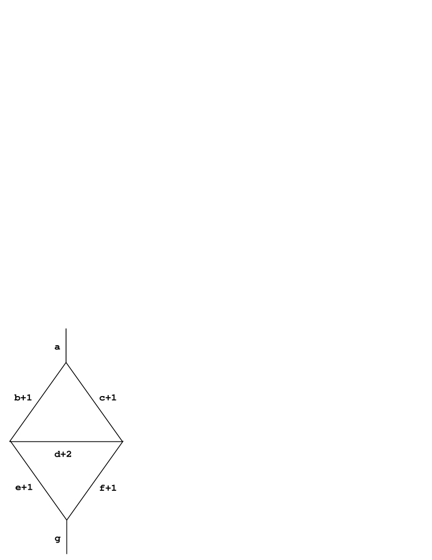
Figure 9: A final state such that all colors have increased

Having chosen a definite final state from all those occuring in [C,C], the next step is to choose how the constraints are smeared (how the Lagrange multipliers are evaluated). I will consider two procedures: vertex smearing and area smearing. Vertex smearing is the procedure used at eqs. (1) and (2): multiply the constraint by the value of the smearing function (Lagrange multiplier) at the vertex which is grasped. In eq. (2), for example, $\rm M_{A}$ is the value of the smearing function at vertex A, and $\rm C_{A}$ is the sum of all terms in the scalar constraint which grasp some pair of edges ending at A. Now that the small loop is extended over an entire triangle, however, perhaps a more appropriate procedure is to use area smearing: multiply the constraint by the average value of M on the triangle, for instance by $\rm M_{bcd}=(M_{B}+M_{C}+M_{D})/3$, for a triangle with sides bcd and vertices BCD. The commutator, eq. (2), would be replaced by

$$[\int MC,\int NC]=(M_{bcd}N_{def}-M_{def}N_{bcd})[C_{bcd},C_{def}]+\cdots,$$ (19)

where $\rm C_{bcd}$ is the sum of all terms in the scalar constraint which grasp a pair of edges in the triangle bcd. Since the functions M and N are arbitrary, the commutator must vanish term by term. Each $\rm[C_{A},C_{B}]=0$ for vertex smearing; and each $\rm[C_{bcd},C_{def}]=0$ for area smearing.

Vertex smearing is easier to check, since $\rm C_{A}$ contains fewer terms than $\rm C_{bcd}$; therefore check vertex smearing first. Let vertex A be the topmost vertex in figure 7; let vertex B be the leftmost vertex, where edges bde meet. Since I want only those grasps which lead to the final state of figure 9, I need to consider only the term in $\rm C_{A}$ which grasps sides bc, and only the term in $\rm C_{B}$ which grasps sides de. The result is

$$[C_{A},C_{B}](figure~{}8)=\cdots+(figure~{}9)[bcde-(d+1)ebc](1/2)^{4}.$$ (20)

The $\rm(1/2)^{4}$ comes from the four color two recoupling factors; all color zero recoupling factors and triangle factors are unity. Only the grasp factors (in the square bracket) are non-zero. They do not cancel, and the commutator is anomalous. It is easy to see why this happens. When the grasp across lines de occurs first ($\rm C_{A}C_{B}$ term in the commutator) the grasp factor is de; whereas when the grasp across lines de occurs second ($\rm-C_{B}C_{A}$ term in the commutator) the grasp factor is (d+1)e, because the prior action of $\rm C_{A}$ has changed the color of edge d to d+1. Obviously this grasp anomaly is likely to occur whenever there is correlation: whenever the action of C at one location (vertex or triangle) changes the colors of the lines at another location. For the general final state there will be recoupling and triangle anomalies as well as grasp anomalies. Once correlation is introduced, anomalies are the rule, rather than the exception.

Now consider area smearing. Consider the $\rm[C_{bcd},C_{def}]$ term. $\rm C_{bcd}$ is a sum of three terms, since the scalar constraint can grasp edges bc, cd, or db. All three grasps can change the b, c, and d sides of figure 8 upward by one unit. Similarly, all three grasps in in $\rm C_{def}$ can change the d, e, and f sides upward by one unit; hence all six terms making up $\rm C_{bcd}$ and $\rm C_{def}$ will lead to the final state of figure 9, and all terms must be kept. Fortunately, again, only grasp factors are non-trivial. The final result is

$$\rm\displaystyle[C_{bcd},C_{def}](figure~{}8)=\cdots$$

$$\rm\displaystyle\;+(figure~{}9)\{[bc+b(d+1)+c(d+1)][ef+ed+fd]$$

$$\rm\displaystyle\;-[ef+e(d+1)+f(d+1)][bc+bd+cd]\}(1/2)^{4}.$$ (21)

This expression is anomalous also.

As discussed in the introduction, it is not entirely clear that imposing freedom from anomalies is a reasonable thing to do. However, one might wish to impose the requirement that the anomalous terms in the commutator are small, in the classical limit, because in the classical, continuum theory a very wide range of fields may be used to carry representations of the diffeomorphism group, including fields which do not satisfy the scalar constraint. Presumably anomalous terms are “small’ if the commutator [C,C] has small matrix elements compared to matrix elements of $\rm C^{2}$, in the limit that all colors a, b, c, $\rm\cdots$ are order n, $\rm n\gg 1$. From eq. (20) or eq. (21), this requirement is satisfied, since

$$[C,C]/C^{2}=O(1/n).$$ (22)

IV Four-dimensional approaches and further discussion

Reisenberger and Rovelli [20] have suggested that a kind of 3+1 dimensional “crossing symmetry” could be used to fix some of the arbitrariness in the scalar constraint. They construct a proper time coordinate T and propagate a spin network from proper time 0 to T using a path integral formalism. Each path is weighted by an exponential $\rm exp[-i\int_{0}^{T}dT^{\prime}H]$, where H is the usual gravitational Hamiltonian, a sum of constraints . They expand the exponential in powers of H, and visualize the action of each power of H on the spin network as follows. (The diagrams are drawn in 2+1 rather than 3+1 dimensional spacetime for ease of visualization, and the vertical direction is the proper time direction T.) Stack figure 2 vertically above figure 1. Figure 1 represents a portion of the spin network at T = 0, before H has acted; figure 2 represents the same spin network at proper time T after H has acted. Connect figures 1 and 2 by three approximately vertical lines. All three lines begin at the “a” vertex of figure 1. One line connects the “a” vertex of figure 1 to the “a” vertex of figure 2; the other two lines connect the “a” vertex of figure 1 to the two new vertices at the ends of the color unity line in figure 2. The action of the scalar constraint therefore introduces a tetrahedron into spacetime: the bottom vertex is the “a” vertex of figure 1; the three vertical edges are the world-line of this vertex and the world lines of the two new vertices introduced by H; the top face is the spin network triangle with edges $\rm(b^{\prime},c^{\prime},1)$ in figure 2. For later reference note that the three vertical edges of this tetrahedron are qualitatively different from the three horizontal edges $\rm(b^{\prime},c^{\prime},1)$. The vertical edges are world-lines of vertices; they are not colored; they are not edges of any spin network.

Any time slice (horizontal slice) through the middle of the tetrahedron will separate it into a “past”, ccontaining one vertex, and a “future”, containing three vertices. Reisenberger and Rovelli call this a (1,3) transition. They argue that 3+1 diffeomorphism invariance should allow one to rotate the tetrahedron in 3+1 dimensional space, or equivalently time-slice the tetrahedron at any angle. This is what they mean by “crossing symmetry”. In particular, consider a slice which would put two vertices in the past and two in the future: by crossing symmetry, H should allow not only (1,3) transitions, but also (2,2) transitions. (In a (2,2) transition the number of vertices does not change, but the way the vertices are coupled does change.)

A (2,2) slice is qualitatively different from a (1,3) slice, however. The (1,3) time slice cuts only the vertical, world line edges of the tetrahedron; the (2,2) slice cuts both world line edges and spin network edges. In short, the tetrahedron is not really 4-D symmetric: its sides are not all equivalent.

Markopoulou and Smolin [21] have proposed a four-dimensional spin network formalism in which the fundamental tetrahedrons are more fully symmetric, because all edges are colored. Markopoulou and Smolin do not use their formalism to determine the form of the scalar constraint. Indeed it would be contrary to their philosophy to do so. In their approach, the classical Einstein-Hilbert action emerges at the end of a long renormalization group calculation. One starts from a microscopic action (as yet unspecified, but presumably highly symmetric). If the initial action is in the right universality class, then the renormalization group calculation yields correlated behavior over macroscopic scales, as required by the classical theory.

Sections I-III of this paper discusses three-dimensional spin networks; but the results of those sections should carry over readily to the 3+1 dimensional approaches just discussed. Presumably the initial microscopic Markopoulou-Smolin action should be chosen so as to affect more than one vertex at a time, insert no edges of color unity. and obey a crossing symmetry (following Reisenberger and Rovelli) .

In order to obtain correlation and eliminate length distortions, I have required that the color unity loop added by the scalar constraint should be pushed outward from the vertex where the constraint initially acts, until the loop fills an entire triangle of the spin network. Consequently the constraint will not change the number of vertices in the spin network (although it can change the number of lines). For example, the uncorrelated scalar constraint action shown in figure 2 has added two new vertices, whereas the correlated action shown in figure 5 adds no new vertices (after recouplings which remove the color unity lines).

To see how the constraint could add a new edge, set d = 0 in figure 2 (no edge present initially). The two bottom vertices are now divalent, but that can be remedied, if desired, by adding new external lines; the valence will not matter. As before, let the constraint act at the top vertex, push the loop down the sides of the triangle, and recouple so as to fill the entire triangle (as in figures three through five, now with d = 0). The d = 0 edge is replaced by $\rm d^{\prime}$ = 1; a new edge has been added.

One could demand that the procedure be modified so that not even a new edge is added. For example, suppose the triangle with edges bcd in figure 2 were part of the larger spin network shown in figure 8. Again set d = 0 and let the scalar constraint act at the upper vertex, but do not stop when the color unity loop has filled the upper half triangle of figure 8; continue to push this color unity loop until it fills the entire diamond. After recouplings such that $\rm b\mbox{$\rm\rightarrow$}b^{\prime},e\mbox{$\rm\rightarrow$}e^{\prime},...$, there is neither a new vertex nor a new edge.

There is some rationale for stopping when the loop has filled only the upper half of the diamond, however: if one thinks of the spin network as triangulating the space, then for pairs of edges which share a common vertex, such as the pair (b,c) in figure 8, there should be a third edge which connects the ends of b and c away from the vertex, so as to form a triangle; otherwise the structure is not rigid, in general. One could say that the network of figure 8 with d = 0 really has a horizontal edge across the middle of the diamond; the edge just happens to have the special color value zero. Put another way, the scalar constraint should leave the number of vertices fixed, while adding enough edges to form a rigid structure. This idea is appealing in its simplicity, but sometimes an idea can be too simple for its own good. Further thought is needed.

Acknowledgements

I would like to thank Lee Smolin for helpful discussions, and Lee Smolin and Abhay Ashtekar for their hospitality while I was a visitor at the Center for Gravitational Physics and Geometry.

References

- [1] C. Rovelli L. Smolin , Spin networks and quantum gravity, Phys. Rev. D55 6099 (1997).
- [2] A. Ashtekar, J. Lewandowski, D. Marolf, J. Mourão, and T. Thiemann, J. Math Phys. (N.Y.) 36 6456 (1995)
- [3] J. Baez, in Knots and Quantum Gravity Oxford University Press, Oxford, 1994.
- [4] for applications of loops to gauge theories in general, see R. Gambini and A. Trias Phys. Rev. D22 1380 (1980); Nucl. Phys. B278 436 (1986)
- [5] C. Rovelli and L. Smolin Nucl. Phys. B442 593 (1995); A. Ashtekar C. Rovelli and L. Smolin Phys. Rev. Lett. 69 237 (1992)
- [6] R. Loll Phys. Rev. Lett. 75 3048 (1995)
- [7] L. Smolin, in Quantum gravity and cosmology edited by J. Pérez-Mercader et. al. , World Scientific, Singapore (1992)
- [8] ; A. Ashtekar and J. Lewandowski, “Quantum theory of geometry II: volume operators”, gr-qc 9711031.
- [9] L. Smolin, “The classical limit and the form of the Hamiltonian constraint in nonperturbative quantum gravity”, gr-qc 9609034
- [10] M.E. Agishtein and A.A. Migdal, Nucl. Phys. B385 395 (1982); J. Ambjorn, J. Jerkiewicz, and Y. Watabiki, J. Math. Phys. 36 6299 (1995)
- [11] T. Thiemann Physics Letters B388 257 (1996); “Quantum spin dynamics” I and II, gr-qc 9606089-90.
- [12] C. Rovelli and L. Smolin Phys. Rev. Lett. 72 446 (1994)
- [13] C. Rovelli, J. Math. Phys (N.Y.) 36 6529 (1995)
- [14] T. Thiemann, “A length operator for canonical quantum gravity”, gr-qc 9606092
- [15] Hojman S.A. Kuchař K. Teitelboim C. 1976 Ann.Phys. (NY) 96 88
- [16] for area and volume operators: C. Rovelli and L. Smolin, Nucl. Phys. B442 593 (1995); A. Ashtekar and J. Lewandowski Class. Quantum Grav. 14 A55 (1997)
- [17] for volume operators: R. De Pietri and C. Rovelli Phys. Rev. D54 2664 (1996); T. Thiemann,“Closed formula for the matrix elements of the volume operator..”, gr-qc 9606091; A. Ashtekar and J. Lewandowski, J. Geom. Phys. 17 191(1995). For a lattice formulation see R. Loll, Nucl. Phys. B460143 (1996). and
- [18] C. Rovelli, L. Smolin Nucl. Phys. B331 80 (1990)
- [19] Louis H. Kauffman and Sóstenes L. Lins, Temperley-Lieb Recoupling Theory and Invariants of 3-Manifolds Princeton University Press, Princeton, New Jersey, 1994
- [20] M. P. Reiseberger and C. Rovelli, Phys. Rev D56 3490 (1997)
- [21] F. Markopoulou and L. Smolin, “Causal evolution of spin networks”, gr-qc 9702025.