The singularity in supercritical collapse of a spherical scalar field

Abstract

We study the singularity created in the supercritical collapse of a spherical massless scalar field. We first model the geometry and the scalar field to be homogeneous, and find a generic solution (in terms of a formal series expansion) describing a spacelike singularity which is monotonic, scalar polynomial and strong. We confront the predictions of this analytical model with the pointwise behavior of fully-nonlinear and inhomogeneous numerical simulations, and find full compliance. We also study the phenomenology of the spatial structure of the singularity numerically. At asymptotically late advanced time the singularity approaches the Schwarzschild singularity, in addition to discrete points at finite advanced times, where the singularity is Schwarzschild-like. At other points the singularity is different from Schwarzschild due to the nonlinear scalar field.

PACS number(s): 04.70.Bw, 04.20.Dw

]

I Introduction

The spherically-symmetric collapse of a scalar field has been studied extensively in the last few years. It was shown that when one changes the value of a parameter which characterizes regular initial data (while freezing the other parameters), there exists a critical value of the parameter beyond which an apparent horizon (and consequently a black hole) forms. For parameters smaller than the critical ones, no stable configurations form, and the field disperses to infinity [1, 2]. Despite the significant advance gained recently in the understanding of dynamical gravitational collapse, the spacetime interior to the apparent horizon has received little attention. In particular, the nature of the spacetime singularity predicted to form inside the black hole in supercritical collapse, remained unresolved.

The linearized scalar-field perturbations of the interior of the Schwarzschild spacetime have been known for two decades now[3]. This leads naturally to the following questions: To what extent is the spacetime singularity in nonlinear collapse similar to the linearly perturbed Schwarzschild singularity? As the backreaction of the scalar field is expected to change the Schwarzschild singularity, what are the features and properties of this singularity? The goal of this paper is to study these questions within the model of the fully nonlinear collapse of a minimally-coupled, self-gravitating, spherically-symmetric, massless, real scalar field. We shall construct a simple analytical model to describe the singularity which evolves in this model, and confront it with fully-nonlinear numerical simulations.

The organization of this paper is as follows. In Section II we present the analytical model and its main conclusions. We find a generic solution for the pointwise behavior at the singularity. This singularity is spacelike, scalar polynomial, and strong. In Section III we describe the numerical simulations and compare these simulations with the predictions of the analytical model. We find full compliance between the analytic results and the numerical simulations. We also study numerically the spatial structure of the singularity. We make some concluding remarks in Section IV.

II Analytical model

The linear perturbation analysis of the interior of the Schwarzschild spacetime with a massless scalar field predicts the scalar field to diverge like $\ln r$ along radial $t={\rm const}$ lines [3]. Here, $r$ is the radial Schwarzschild coordinate defined such that circles of radius $r$ have circumference $2\pi r$ ($r$ is timelike inside the black hole) and $t$ is normal to $r$ ($t$ is spacelike inside the black hole). (There is a gauge freedom in $t$—see below.) Therefore, near the singularity at $r=0$ one would no longer expect the linear solution to be valid. Rather, one would expect the backreaction on the metric to be significant. Consequently, in order to describe the singularity in this model one would need to solve the fully nonlinear Einstein-Klein-Gordon equations. Moreover, in the case of dynamical collapse the formation of the singularity is a nonlinear effect, and no linear perturbation analysis can be made in the first place.

The analytical solution of the full Einstein-Klein-Gordon equations turns out to be very difficult even in spherical symmetry. However, the analysis of linearized perturbations of the Schwarzschild singularity [3] finds that at large values of $t$ the interior regions tend to a state which depends only on $r$. For any finite $r$ near the singularity the linear spherical scalar field vanishes like $t^{-3}$ at large $t$. One would expect, therefore, the deviations from Schwarzschild to be small at $t\to\infty$ (at finite $r$). It looks reasonable, therefore, to look for a simplified analytical model where dynamical variables depend only on $r$ also in the nonlinear case, at least for large $t$.

Let us consider the general homogeneous spherically-symmetric line-element

$$\,ds^{2}=h(r)\,dt^{2}+f(r)\,dr^{2}+r^{2}\,d\Omega^{2},$$ (1)

where $\,d\Omega^{2}=\,d\theta^{2}+\sin^{2}\theta\,d\phi^{2}$ is the metric on the unit 2-sphere. The field equations are given by

$$\left(f^{\prime}r+f^{2}-f\right)/\left(fr^{2}\right)=\Phi^{\prime 2}$$ (2)

$$\left(h^{\prime}r-hf+h\right)/\left(hr^{2}\right)=\Phi^{\prime 2}$$ (3)

$$\left[\left(h^{2}\right)^{\prime}\,\left(f-\frac{1}{2}rf^{\prime}\right)+2rf\,\left(hh^{\prime\prime}-\frac{1}{2}h^{\prime 2}\right)-2f^{\prime}h^{2}\right]$$ (4)

$$/\left(4rfh^{2}\right)=-\Phi^{\prime 2}$$ (5)

and by the Klein-Gordon equation $\nabla_{\mu}\nabla^{\mu}\Phi=0$ for the scalar field $\Phi$. Here, a prime denotes differentiation with respect to $r$. Because of the spherical symmetry and the homogeneity, the Klein-Gordon equation is readily integrated to

$$\Phi^{\prime}(r)=d\;\sqrt{\left|f/\left(hr^{4}\right)\right|},$$ (6)

where $d\neq 0$ is an integration constant, which will be shown below to be arbitrary, and to describe a pure gauge mode. We next use Eq. (6) to eliminate the scalar field from Eqs. (2)–(5). We obtain

$$f^{\prime}r+f^{2}-f+d^{2}\frac{f^{2}}{hr^{2}}=0$$ (7)

$$h^{\prime}r-hf+h+d^{2}\frac{f}{r^{2}}=0$$ (8)

$$h^{\prime\prime}-\frac{h^{\prime 2}}{2h}+\frac{1}{r}\left(h^{\prime}-h\frac{f^{\prime}}{f}\right)-\frac{h^{\prime}f^{\prime}}{2f}-2d^{2}\frac{f}{r^{4}}=0.$$ (9)

We assume a formal series expansion for $f,h$, and seek a generic solution for a spacelike singularity. We find that

$$f(r)= - \left(\beta+1\right)Cr^{\beta+2}-\frac{\left(\beta+1\right)^{2}\left(3\beta+4\right)}{\left(\beta+2\right)^{2}}C^{2}r^{2\beta+4}$$ (10)

$$+ O\left(r^{3\beta+6}\right)$$ (11)

$$h(r)=d^{2}Cr^{\beta}+d^{2}\frac{\beta\left(\beta+1\right)}{\left(\beta+2\right)^{2}}C^{2}r^{2\beta+2}+O\left(r^{3\beta+4}\right)$$ (12)

$$\Phi(r) = \sqrt{\beta+1}\,\ln r+\frac{\sqrt{\beta+1}\,\left(5\beta^{2}+12\beta+6\right)}{\left(\beta+2\right)^{3}}Cr^{\beta+2}$$ (13)

$$+ O\left(r^{2\beta+4}\right).$$ (14)

Here, $\beta\geq-1$ and $C>0$ are free parameters. This solution suggests the the complete formal series expansion is of the form

$$\left[\begin{array}[]{c}f(r)\\ h(r)\end{array}\right]=\left(\begin{array}[]{c}1\\ d^{2}/r^{2}\end{array}\right)\sum_{n=1}^{\infty}\left[\begin{array}[]{c}a_{n}^{f}\left(\beta,C\right)\\ a_{n}^{h}\left(\beta,C\right)\end{array}\right]\,r^{(\beta+2)n}.$$ (15)

It can be shown that the expansion coefficients $a_{n}^{f,h}$ can be found uniquely for any $n$ [4]. For the scalar field we find

$$\Phi(r)=\sqrt{\beta+1}\,\ln r+\sum_{n=1}^{\infty}a_{n}^{\Phi}\left(\beta,C\right)\,r^{(\beta+2)n}.$$ (16)

We note that because the Klein-Gordon equation is linear in the scalar field $\Phi$, whereas the Einstein equations (2)–(5) are quadratic in $\Phi$, the overall sign in Eq. (14) is arbitrary.

We next discuss the genericity of the solution. The notion of a general solution for a system of nonlinear differential equations is not unambiguous. However, one can count the number of free parameters in the solution, and compare it with the expected number. If these two numbers are equal, than the solution is generic, in the sense that it captures a volume of non-zero measure in solution space. From the physical point of view one would expect two free parameters (one because of Birkhoff’s theorem and one due to the scalar field). Apparently, our solution above has three free parameters, namely, $d^{2},C,\beta$. However, the parameter $d^{2}$ reflects a pure gauge mode. That is, one has the freedom to re-scale the coordinate $t$ by $t\to t^{\prime}=T(t)$. In such a gauge transformation $d^{2}$ is changed (and in general the parameter $d^{2}$ can be replaced by any smooth function of $t$) without changing the physical content of the solution. (The parameter $d^{2}$ remains a constant parameter which does not depend on $t$ for the class of transformations $t\to t^{\prime}=pt+q$ for constant $p$ and $q$.) Thus, the scalar field (16) and curvature scalars below are independent of $d^{2}$. Consequently, our solution depends on two physical degrees of freedom ($\beta$ and $C$), and is therefore generic.

The curvature can be described, say, by curvature scalars. We find that to the leading order in $r$

$$R=-\frac{2}{C}\,r^{-(\beta+4)}$$ (17)

$$R_{\mu\nu}R^{\mu\nu}=\frac{4}{C^{2}}\,r^{-(2\beta+8)}$$ (18)

$$R_{\mu\nu\rho\sigma}R^{\mu\nu\rho\sigma}=4\frac{2\beta^{2}+2\beta+3}{\left(\beta+1\right)^{2}C^{2}}\,r^{-(2\beta+8)}.$$ (19)

Here, $R$ is the Ricci scalar, $R_{\mu\nu}$ is the Ricci tensor, and $R_{\mu\nu\rho\sigma}$ is the Riemann-Christoffel tensor. From these expressions the singularity is clearly scalar polynomial. We next show that it is strong in the Tipler sense [5], namely, any extended physical object will unavoidably by crushed to zero volume upon hitting the singularity. Let us denote by $x^{0}$ the coordinate tangent to the worldline of an object infalling along a radial $t={\rm const}$ worldline, and by $\tau$ its proper time, set such that $\tau=0$ at $r=0$. Then, the $(00)$ tetrad component of the Ricci tensor, to the leading order in $\tau$, is given by

$$R_{(0)(0)}(\tau)=8\,\frac{\beta+1}{(\beta+4)^{2}}\,\tau^{-2}.$$ (20)

By Ref. [6], Eq. (20) implies that the singularity is strong in the Tipler sense, as

$$\int_{\tau_{0}}^{\tau}\,d\tau^{\prime}\int_{\tau_{0}}^{\tau^{\prime}}\,d\tau^{\prime\prime}R_{(0)(0)}(\tau^{\prime\prime})$$ (21)

diverges logarithmically at $\tau=0$.

Finally, let us define a ‘tortoise’ coordinate $r_{*}$ by $g_{r_{*}r_{*}}=-g_{tt}$. Then, null coordinates are defined by $t=(v-u)/2$ and $r_{*}=(v+u)/2$, with ingoing $v$ and outgoing $u$. For a certain outgoing ray $u=u_{0}\equiv\rm{const}$ which runs into the spacelike singularity, the latter is hit at some finite value of advanced time $v=v_{*}$ (see Fig. 1). (Future null infinity is located at $v=\infty$.) We then find, to the leading order in $v_{*}-v$, that

$$r(u_{0},v)=\left[d^{2}/(\beta+1)\right]^{1/4}\;(v_{*}-v)^{1/2}.$$ (22)

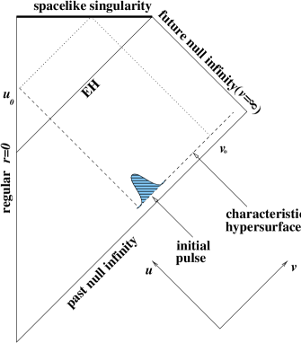
FIG. 1.: The Penrose diagram of the simulated spacetime. Prior to the characteristic hypersurface the geometry is Minkowskian. Due to the supercritical initial pulse a black hole is formed. For an outgoing null ray at $u_{0}$ the spacelike singularity is hit at $v=v_{*}$. Future null infinity is at $v=\infty$.

We note that as this model is homogeneous (the metric functions and the scalar field depend only on $r$), it actually describes just the pointwise behavior of the singularity. In general, the singularity is expected to depend not only on $r$ but also on $t$. This dependence on $t$ cannot be captured by our homogeneous model. The inhomogeneities will be studied therefore numerically.

III Numerical simulations

A Initial data

We constructed a numerical code based on double-null coordinates and on free evolution of the dynamical variables [7]. The code is stable and converges with second order (see below). We specify regular initial data on the characteristic hypersurface, which is located at $u=u_{i}$ and $v=v_{i}$ (see Fig. 1). Prior to the initial pulse the geometry is Minkowskian. Then, due to the nonlinear scalar field, the geometry is changed, and an apparent horizon forms. At late advanced time ($v\to\infty$) the apparent horizon coincides with the event horizon (EH), and the black hole approaches asymptotically the (external) Schwarzschild black hole [7].

The details of the collapse model, the formulation of the characteristic problem, and the description of the code are given in Ref. [7]. Here, we shall describe them very briefly. The null coordinates $u,v$ are defined such that $v=r$ and $u=(r-r_{0})/r_{u0}$ on the characteristic hypersurface, where $r_{0}=r(u_{i},v_{i})$. (Note that this coordinate $v$ is not identical to the coordinate $v$ in Eq. (22).) The initial data we specify are the following. The scalar field vanishes everywhere on the characteristic hypersurface, except for the compact interval $v_{1}<v<v_{2}$, where the scalar field has the form $\Phi(u_{i},v)=A\sin^{2}[\pi(v-v_{1})/(v_{2}-v_{1})]$. The rest of the initial data are chosen such that the constraint equations are satisfied on the characteristic hypersurface. The parameter which we vary is the amplitude $A$ in $\Phi(u_{i},v)$. For small values of $A$ the initial data are subcritical, and no black hole forms. For large values of $A$, however, the initial data are supercritical, and a black hole forms. We shall discuss below only the latter case, namely, the internal structure of the black hole which forms in supercritical collapse. In the simulations described below the free parameters in the initial data are chosen to be $r_{0}=10$, $r_{u0}=-1/4$, $v_{1}=10$, $v_{2}=16$, and $A=0.29$. (These initial data correspond to a Minkowskian geometry for $v<v_{1}$ or $u<u_{i}$.) These initial data result with a black hole with final mass $M_{f}\approx 4.02$. The value of $M_{f}$ can be easily determined from the value of $r$ at the apparent horizon: $r$ at the apparent horizon is just twice the mass of the black hole. Figure 2 displays the mass of the black hole as a function of advanced time $v$. For $v<11.4$ the domain of integration does not intersect the apparent horizon, and therefore the mass of the black hole is not shown. (We note that because our code does not include the origin, we cannot find the apparent horizon of black holes with infinitesimal mass.) We find results similar to those reported below also for other values of supercritical initial-data parameters. (We have also studied the case of nonlinear perturbations of a pre-existing Schwarzschild black hole, by specifying the appropriate initial data. In this case we find that the properties of the singularity are similar to those found in supercritical collapse. In the latter case, however, the dynamical evolution of the spacetime geometry brings out the nonlinear aspects in a sharper way, and therefore we shall describe here only this latter case.)

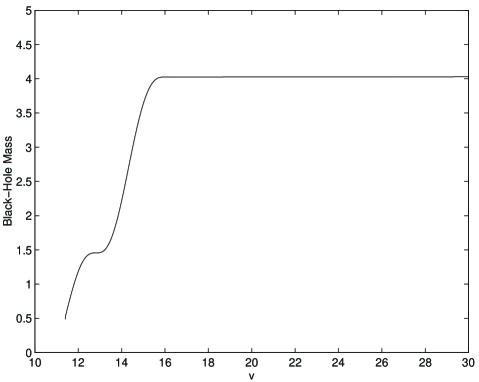
FIG. 2.: Black hole mass as function of advanced time $v$. The mass is evaluated by means of the value of $r$ at the apparent horizon.

The only changes we introduced in the code which is described in Ref. [7] are related to a careful approach to $r=0$: First, with uniform spacings of the grid in advanced time one would hit the singularity within a finite integration time and subsequently the code would crash. (However, one still needs to preserve the dynamical refinement of the mesh in retarded time.) We resolve this difficulty by checking the expected distance (in advanced time) to the singularity on the last outgoing null ray of the grid for each advanced-time step by means of the above analytical results (11) and (12). We then change the advanced-time step accordingly, such that crashing into the singularity is avoided, and in principle the code can run forever. (In practice, because of the floating-point arithmetic limits of the machine the approach to the singularity is limited. However, one can approach $r=0$ sufficiently close to infer the asymptotic behavior from the simulation.) Second, one would like to study the fields approaching different points along the singularity. Namely, for different values of $v_{*}$. This can be done in the following way. In Ref. [7] we introduce a procedure called “chopping”, which is nothing but excision of the domain of integration slightly beyond the apparent horizon. Here, as we are interested in approaching the spacelike singularity at $r=0$, this procedure is performed only up to some finite value of advanced time $v_{c}$. The later $v_{c}$, the larger $v_{*}$, and the closer we arrive to the vertex point in the spacetime diagram 1 which is at $v_{*}\to\infty$. This way we can arrive at different points along the spacelike singularity, and study the spatial dependence of the fields at the singularity.

B Numerical simulations of the black hole interior

We perform numerical simulations of the interior of the created black hole. Let us first confront the predictions of the homogeneous model described in Sec. II with the pointwise behavior at the singularity as obtained from the fully-nonlinear and inhomogeneous numerical simulations. Then, we shall also study the phenomenology of the spatial structure of the singularity numerically.

1 The pointwise behavior

We first discuss the behavior of the metric functions near the singularity. In double null coordinates the metric function $g_{uv}$ is expected from Eq. (12) to behave near the singularity like $g_{uv}\propto r^{\beta}$ to leading order in $r$, because $g_{tt}=2(\,\partial u/\,\partial t)(\,\partial v/\,\partial t)g_{uv}$, and $\,\partial v/\,\partial t=1=-\,\partial u/\,\partial t$. (The gauge freedom in $t$ is manifested just in a multiplicative factor, and not in the exponent $\beta$ which concerns us here.) Figure 3 (A) displays $F=-2g_{uv}$ along an outgoing null ray at $u=u_{0}$, as a function of $r$. The straight line in Fig. 3 (A) indicates a power-law behavior. The asymptotic power-law behavior is checked more carefully in Fig. 3 (B), which shows the local power index of $F$ as a function of $r$. This local power index is nothing but the exponent $\beta$ in Eq. (12). As $\beta$ approaches asymptotically a constant value, the power-law behavior is verified.

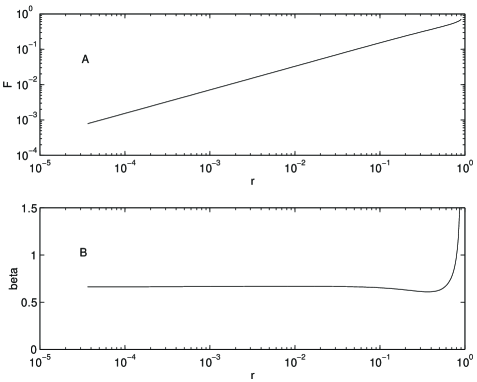
FIG. 3.: The behavior of the metric function $g_{uv}$ along an outgoing null ray: (A) $F=-2g_{uv}$ as a function of $r$. (B) the behavior of the local power index of $F$ as a function of $r$.

The behavior of the metric function $r(u,v)$ is shown in Fig. 4 (A), which displays the distance from the singularity in terms of advanced time $v_{*}-v$, as a function of $r$ along the same outgoing null ray as in Fig. 3 (at $u=u_{0}$). Again, the straight line indicates a power-law behavior, whose local index is displayed in Fig. 4 (B). From Eq. (22) this power-law index is expected to approach asymptotically a value of $2$. This is indeed found numerically, within a numerical error of $5\times 10^{-3}$.

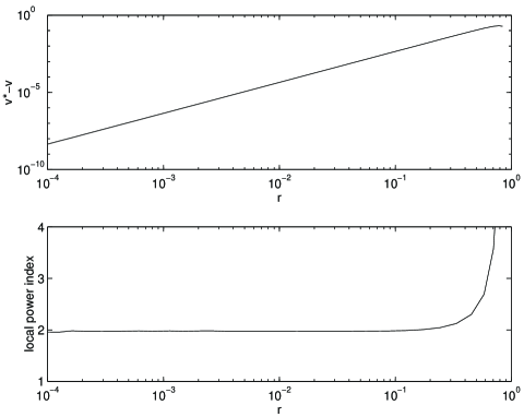
FIG. 4.: (A) $v_{*}-v$ as a function of $r$. (B) The local power index in (A) as a function of $r$.

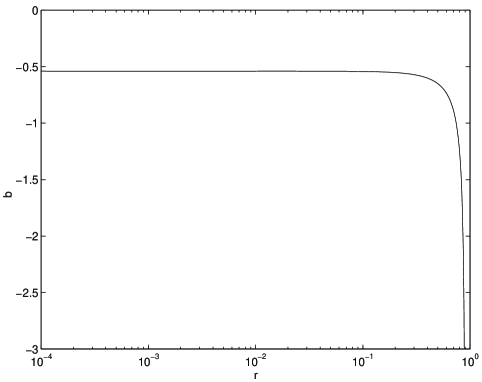
FIG. 5.: The value of $b=-1/(2r_{,u}r_{,v}r^{2})$ as a function of $r$.

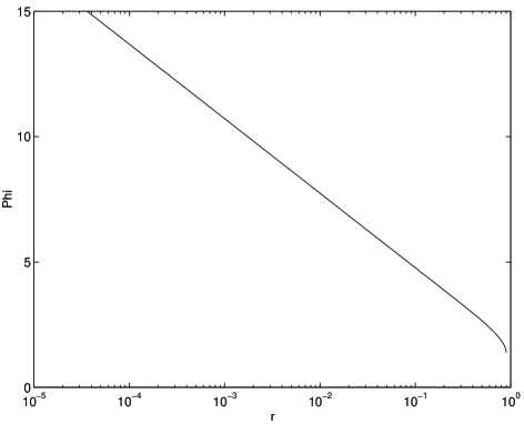
FIG. 6.: The scalar field $\Phi$ as a function of $r$.

Another prediction of the homogeneous model related to the metric functions is that $g_{rr}/g_{uv}\propto r^{2}$, to the leading order in $r$. Let us now find the analogue of this relation in the inhomogeneous case, and compare the homogeneous and inhomogeneous cases numerically. First, in Schwarzschild coordinates $g^{\mu\nu}\,\nabla_{\mu}r\,\nabla_{\nu}r$ is readily shown to equal $g^{rr}$. In double-null coordinates, $g^{\mu\nu}\,\nabla_{\mu}r\,\nabla_{\nu}r=2g^{uv}r_{,u}r_{,v}=-(4/F)r_{,u}r_{,v}$, where $F(u,v)=-2g_{uv}(u,v)$. Combining these two expressions, one obtaines $g_{rr}(u,v)=-F/(4r_{,u}r_{,v})$. Consequently, we find that $g_{rr}/g_{uv}=-1/(2r_{,u}r_{,v})$. Figure 5 shows $b=-1/(2r_{,u}r_{,v}r^{2})$ along the same outgoing null ray at $u_{0}$, as a function of $r$. This ratio approaches asymptotically a constant value, which confirms this prediction of the homogeneous model. (The gauge freedom in $t$, which is translated here into a gauge freedom in both $u$ and $v$, changes here just the value of this constant.)

The behavior of the scalar field $\Phi$ along $u=u_{0}$ is shown in Fig. 6. The straight line here indicates a logarithmic divergence of $\Phi$, as implied by Eq. (14).

The stability and convergence of the code are demonstrated in Figs. 7 and 8. Figure 7 shows a magnified portion of Fig. 3 and Fig. 8 shows a magnified portion of Fig.  6 for different values of the grid parameter $N$, namely, for $N=20,40$, and $80$, where $N$ is the (initial) number of grid points per a unit interval in both the ingoing and outgoing directions. The behavior in the two figures clearly indicates stability and convergence with second order.

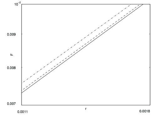
FIG. 7.: The metric function $F$ as a function of $r$ for three values of the grid parameter ($N=20,40,80$); Dashed-dotted: $N=20$, dashed: $N=40$, and solid line: $N=80$.

The homogeneous model also implies that $\beta$ appears in two places, which numerically are independent. Namely, in the exponent of $h(r)$ [given by Eq. (12)] and in the amplitude of the scalar field [given by Eq. (14)]. Figure 9 shows the relation of these two values for $\beta$ for two differrent outgoing null rays: The top panel shows the values of $\beta$ for the two null rays as determined from Eq. (12) as functions of $r$, and the bottom panel the ratio of the two expressions for $\beta$ for the two outgoing rays, again as functions of $r$. We chose here the two outgoing null rays to be such that for one of them $\beta$ is positive and for the other $\beta$ is negative. The lower panel in Fig. 9 indicates that the two expressions for $\beta$ are asymptotically equal to within one part in $10^{4}$.

The last prediction of the homogeneous model we test with the numerical simulations is the behavior of the Ricci curvature scalar given in Eq. (17). The top panel in Fig. 10 displays the behavior of the Ricci curvature scalar $R$ along the same outgoing null ray as the data in Figs. 3–8, as a function of $r$. The value of $R$ can most easily be evaluated from the right hand side of the Einstein equations: The Einstein-Klein-Gordon equations are $R_{\mu\nu}=2\Phi_{,\mu}\Phi_{,\nu}$, and the Ricci scalar is simply given by $R=2g^{\mu\nu}\Phi_{,\mu}\Phi_{,\nu}$, which in double-null coordinates and spherical symmetry reduces to

$$R=-\frac{8}{F}\Phi_{,u}\Phi_{,v}.$$ (23)

In order to evaluate the expression (17) for $R$ we need first to express $C$. This can be done by comparing our result that $g_{rr}=-F/(4r_{,u}r_{,v})$ with the leading order in $r$ expression for $f$ from (11). We find that to the leading order in $r$

$$C=\frac{1}{4}\,\frac{F}{\beta+1}\,\frac{1}{r_{,u}r_{,v}}\,r^{-(\beta+2)}.$$ (24)

The bottom panel of Fig. 10 shows the ratio of $R$ as calculated from Eq. (23) and $R$ as calculated from Eqs. (17) and (24), as a function of $r$. This ratio asymptotically deviates from unity by $3\times 10^{-4}$, despite the growth of $R$ by a factor of order $10^{20}$.

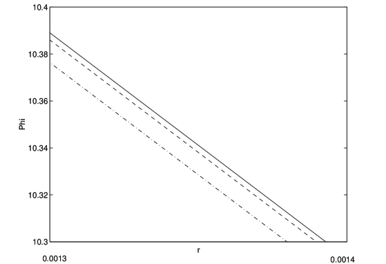
FIG. 8.: The scalar field $\Phi$ as a function of $r$ for three values of the grid parameter ($N=20,40,80$); Dashed-dotted: $N=20$, dashed: $N=40$, and solid line: $N=80$.

2 The inhomogeneous behavior

The inhomogeneous behavior near the singularity can be demonstrated by the variation of $\beta$ along the singularity. Namely, $\beta$ is no longer a parameter, but $\beta=\beta(t)$. [We would also expect $C=C(t)$.] Another issue which can be studied numerically is the overall sign issue of the scalar field. This sign is of importance, as its meaning is related to the divergence of $\Phi$ to $+\infty$ (for a minus sign) or to $-\infty$ (for a plus sign). We find that there are regions where $\Phi$ diverges to $+\infty$ and regions where $\Phi$ diverges to $-\infty$. Figure 11 (A) shows $\beta$ as a function of $v_{*}$. For low values of $v_{*}$, $\beta$ is positive. Then, $\beta$ changes its sign, arrives at a minimum at which its value is $-1$, increases again, and finally, at late $v_{*}$, approaches asymptotically the value of $-1$. Although the numerical simulations indicate that $\beta$ has at least two more local minima, because of the numerical noise it is hard to locate them accurately. This can be done, however, in terms of the scalar field. The sign of the scalar field can be determined from $c=r\Phi_{,r}$, which, to the leading order in $r$ is $\mp\sqrt{\beta+1}$. Clearly, whenever $c(v_{*})$ vanishes with a non-vanishing spatial gradient (namely, with $\,\partial c/\,\partial v_{*}\neq 0$), $\beta$ has a local minimum with a value of $-1$. From Figs. 11 (B), (C), and (D) this happens at $v_{*}=13.4$, $22.5$, and $66.4$. We note that these values of $v_{*}$ are not the same as the values of $v$ along the EH where the quasinormal modes have their extrema or vanish. However, they may be related to the quasinormal ringing, as their frequencies are similar. It is hard to quantify this and establish the hypothetical relation between the two oscillations, as we do not have enough cycles of the oscillations of $c$ on the singularity. Yet, Fig. 11 suggests that $c$ oscillates a number of times before it approaches a vanishing value for $v_{*}\to\infty$. In Fig. 11 (B), (C), and (D) the abscissae were chosen to overlap, such that one could infer the overall behavior.

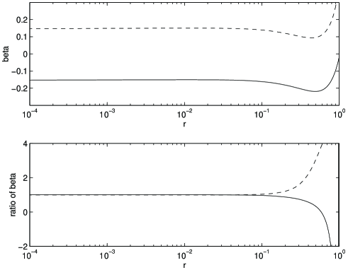
FIG. 9.: Top panel: The values of $\beta$ for two outgoing null rays as functions of $r$. Bottom panel: The ratio of $\beta$ as determined from the exponent in $g_{uv}$ and as determined from the amplitude of the scalar field $\Phi$ for the same two outgoing null rays.

We find, that for a number of discrete points at finite values of $v_{*}$, $\beta=-1$. From Eq. (14) the scalar field $\Phi$ vanishes at these points. One could therefore ask, to what extent the singularity at these points is similar to the Schwarzschild singularity. Let us assume, that in the fully inhomogeneous case the leading order for the metric functions and the scalar field are given by the same form as the leading terms in the homogeneous case, except that the free parameters are replaced by functions of $t$. (Note that higher order terms will have a different form in the inhomogeneous case.) Then, in order that the singularity will be Schwarzschild-like at these points, both the scalar field and its gradient need to vanish there. The gradient of $\Phi$ will vanish only if $\,\partial\beta/\,\partial t$ vanishes. To see if indeed $\,\partial\beta/\,\partial t=0$ at the local minima of $\beta$ let us consider the neighborhood of the first minimum of $\beta(v_{*})$. Figure 12 shows $\beta$ as a function of $v_{*}$ near this first minimum. Figure 12 suggests that indeed $\,\partial\beta/\,\partial t=0$ at the minimum, and consequently the singularity is expected to be Schwarzschild-like there, in the sense that at least the leading order for the scalar field and its gradient vanish there, and $\beta=-1$ as in Schwarzschild. Of course, one would need to consider also higher-order terms in order to study their contribution to the scalar field and to the geometry in an inhomogeneous model for a more detailed comparison of the singularity at these points and the Schwarzschild singularity.

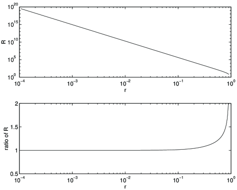
FIG. 10.: Top panel: The behavior of the Ricci scalar $R$ as a function of $r$. Bottom panel: The ratio of $R$ as determined from the fully nonlinear and inhomogeneous numerical simulations and the value of $R$ as determined from the homogeneous model as a function of $r$.

Another point to be made here is related to the limit $v_{*}\to\infty$. At this limit $\beta$ approaches a value of $-1$, and the spatial gradient of $\beta$ vanishes. This is evident from the behavior of $c$ for large $v_{*}$. Consequently, the singularity asymptotically approaches the Schwarzschild singularity at late $v_{*}$. This conclusion agrees wih the conclusion drawn from the linear analysis in Ref. [3]. However, for any finite $v_{*}$ (except for the discrete points for which the scalar field and its gradient vanish on the singularity) $\beta\neq-1$. This means that the scalar field does not vanish on the singularity, and by its backreaction on the geometry the latter is not Schwarzschild. The deviation of the geometry from Schwarzschild is expected, however, to be small for small $\beta+1$, and decrease with growing $t$. In this sense the nonlinear numerical simulations confirm (at least in this model) the dictum of Doroshkevich and Novikov [3] that “a black hole has hair neither outside nor inside.”

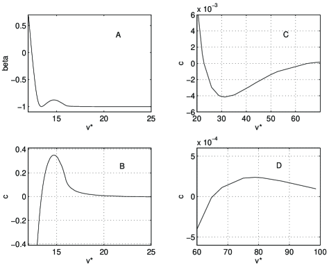
FIG. 11.: (A) $\beta$ as a function of $v_{*}$ along the spacelike singularity. (B), (C), and (D): $c=r\Phi_{,r}$ as a function of $v_{*}$ along the spacelike singularity, for different sections of the latter.

IV Concluding remarks

We remarked above that in order to study the structure of the singularity in this model without the simplifying assumption of homogeneity, one could perhaps replace the free parameters in the solution with functions of $t$. If this were indeed the case, the leading terms are expected to retain their form. However, the higher-order terms in the solution will not. This is due to the appearance of non-vanishing spatial derivatives in the Einstein-Klein-Gordon equations. The solution of the full inhomogeneous equations looks like a formidable challenge even in the special case of spherical symmetry and a scalar field.

Another point concerning the scalar field is related to its serving as a model for a dynamical physical field. The scalar field was introduced as a toy model, because it has a radiative mode in spherical symmetry. In the more realistic case of gravitational waves the field does not have radiative modes in spherical symmetry, and therefore has no non-trivial dynamics. One could ask the following. To what extent do the spherical symmetry and the scalar field capture the essential dynamics of realistic black holes with vacuum perturbations, or the dynamical collapse of spinning fields? Realistic spinning black holes are known to have a Cauchy horizon, which is expected to transform into a null weak singularity [8]. We have shown that in the model of the collapse of a spherical scalar field a spacelike singularity evolves. Will this be the case also in the collapse of gravitational waves? Although as yet there is no answer to this question, we could consider the model of the nonlinear perturbations of a spherical scalar field of a Reissner-Nordström black hole. In this model one also has a Cauchy horizon in the unperturbed spacetime, and one can show that indeed a spacelike singularity evolves [9, 10, 4, 11, 12]. It turns out that there are some important differences between the spacelike singularity we find here (with vanishing electric charge) and the spacelike singularity in the model with charge, despite the similarity of the formal series expansions. First, the parameter $\beta$, which we find here to be greater than $-1$, is restricted to positive values in the presence of charge. Second, we find in the uncharged case that in the limit $v_{*}\to\infty$ the parameter $\beta\to-1$. In the charged case $\beta$ grows very rapidly for large $v_{*}$, and it is reasonable to expect it to diverge as $v_{*}\to\infty$. This difference in the asymptotic behavior of $\beta$ can perhaps be attributed to the following. In the uncharged case as $v_{*}\to\infty$ the outgoing Eddington-like coordinate $u_{e}\to-\infty$. However, because of the presence of the Cauchy horizon in the charged case, the limit $v_{*}\to\infty$ corresponds to a finite value of $u_{e}$. The infinite range of retarded time in the uncharged case acts to infinitely redshift the fields, an effect which does not have an analogue in the charged case.

FIG. 12.: $\beta$ as a function of $v_{*}$. The circles are the data from the numerical simulations, and the solid line is a linear interpolation of these data.

Finally, one might worry about the role that the scalar field plays in this model. Scalar fields are notorious for being related to peculiar phenomena. For example, scalar fields are known to destroy the oscillatory nature of the BKL singularity [13]. Therefore, even though we find the singularity with a spherical scalar field (both in the uncharged and charged cases) to be monotonic, one perhaps could not infer from that on whether the (as yet hypothetical) spacelike singularity inside spinning black holes is monotonic or oscillatory.

REFERENCES

- [1] M. W. Choptuik, Phys. Rev. Lett. 70, 9 (1993).
- [2] For a recent review see C. Gundlach, To appear in Adv. Theor. Math. Phys. and gr-qc/9712084.
- [3] A. G. Doroshkevich and I. D. Novikov, Zh. Eksp. Teor. Fiz. 74, 3 (1978) [Sov. Phys. JETP 47, 1 (1978)].
- [4] L. M. Burko, in Internal structure of black holes and spacetime singularities, edited by L. M. Burko and A. Ori (Institute of Physics, Bristol, 1997).
- [5] F. J. Tipler, Phys. Lett. A 64, 8 (1977).
- [6] C. J. S. Clarke and A. Królak, J. Phys. Geom. 2, 127 (1985), proposition 5.
- [7] L. M. Burko and A. Ori, Phys. Rev. D 56, 7820 (1997).
- [8] A. Ori, Phys. Rev. Lett. 68, 2117 (1992).
- [9] M. L. Gnedin and N. Y. Gnedin, Class. Quantum Grav. 10, 1083 (1993).
- [10] P. R. Brady and J. D. Smith, Phys. Rev. Lett. 75, 1256 (1995).
- [11] L. M. Burko, Phys. Rev. Lett. 79, 4958 (1997).
- [12] L. M. Burko and A. Ori, in preparation.
- [13] V. A. Belinskii and I. M. Khalatnikov, Zh. Eksp. Teor. Fiz. 63, 1121 (1972) [Sov. Phys. JETP 36, 591 (1973)].