Abstract

We present two statistical tests for periodicities in the time series. We apply the two tests to the data taken from Glasgow prototype interferometer in March 1996. We find that the data contain several very narrow spectral features. We investigate whether these features can be confused with gravitational wave signals from pulsars.

Searching data for periodic signals

1 Introduction

The work presented here was motivated by an analysis of Gareth Jones [1] of the data taken from Glasgow prototype in 1996. His visual inspection of the periodogram of the data revealed presence of 3 very narrow (1 bin wide) significant spectral features.

2 Statistical tests for periodicities in the data using the discrete Fourier transform

A standard method to search the time series for periodic signals is to perform the Fourier transform (FT) of the series and examine the modulus of FT for significant values. Let $x_{n}$ be a real-valued discrete time random process given at equally spaced intervals $\Delta t$ so that the sampling frequency $f_{s}$ is equal to $1/\Delta t$. Let the number of samples of $x_{n}$ be $N$ and let us assume for simplicity that $N$ is even. The periodogram $P(f)$, $f\geq 0$, of $x_{n}$ is defined by

$$P(f)=\frac{1}{N}\left|\sum^{N-1}_{n=0}x_{n+1}\exp^{-i2\pi\frac{f}{f_{s}}n}\right|^{2}.$$ (1)

At Fourier frequencies $f_{k}=\frac{k}{N}f_{s}$, $k=0,1,...,N/2$ the quantity in the modulus is the discrete Fourier transform (DFT) of the time series (for non-negative frequencies) and can effectively be evaluated by means of the fast Fourier transform (FFT) algorithm. For the case when $x_{n}$ are uncorrelated and drawn from a Gaussian distribution with zero mean and variance $\sigma^{2}$ and consquently that random variables $P(f_{k})$ are exponentially distributed and independent, Fisher, in a celebrated paper [2], derived a mathematically exact test for the presence of a periodic signal in the data based on the statistics

$$g=\frac{\max_{1\leq k\leq N/2-1}[P(f_{k})]}{\sum^{N/2-1}_{j=1}P(f_{j})},$$ (2)

where $\max_{1\leq k\leq N/2-1}$ means maximum taken over the values of the periodogram evaluated at Fourier frequencies for $k=1,...,N/2-1$. Fisher’s test is the most powerful test against simple periodicities i.e., where the alternative hypothesis is that there exists a periodicity at only one Fourier frequency. Usually there maybe many periodic signals in the data and the number of them may be unknown. For this case Siegel [3] proposed a test based on large values of the periodogram with statistics

$$T=\sum^{N/2-1}_{k=1}\left(\frac{P(f_{k})}{\sum^{N/2-1}_{j=1}P(f_{j})}-\lambda g_{o}\right)_{+},$$ (3)

where $g_{o}$ is the critical value for Fisher’s statistics, $\lambda$ is a parameter such that $0<\lambda\leq 1$, and subscript $+$ denotes the positive part. When $\lambda=1$ Siegel’s test $T>0$ is equivalent to Fisher’s test. Siegel derived exact probability distribution for his statistics. By means of the Monte Carlo simulations he found that for $\lambda=0.6$ his test was only slightly less powerful than Fisher’s test when one periodic signal is present in the data but it was substantially more powerful when 2 or 3 periodic signals were present.

In practice none of the assumption about the time series required for Fisher’s and Siegel’s test are met. The time series may consist of non-Gaussian correlated random variables and moreover the time series may be non-stationary. For stationary processes (not necessarily Gaussian) with continuous spectral density it can be shown (under fairly mild conditions) that asymptotically (i.e. as $N\rightarrow\infty$) periodogram values are independent and exponentially distributed with probability density function (pdf) $p$ given by

$$p[P(f)]=\frac{\exp^{-\frac{P(f)}{S(f)}}}{S(f)},$$ (4)

where $S(f)$ is two-sided spectral density function [4]. The main difficulty in using the above pdf is that usually the spectral density is unknown and has to be estimated from the data itself. We can however obtain an approximate test as follows. Take $L$ blocks of $R$ consequtive values of periodogram evaluated at $M=L\times R$ Fourier frequencies. Consider the following statistics for each block l.

$$g^{\prime}_{k}=\frac{P(f_{k})/S(f_{k})}{\frac{1}{R}\sum^{lR}_{j=(l-1)R+1}P(f_{j})/S(f_{j})}.$$ (5)

Asymptotically $\max[g^{\prime}_{k}]$ has the same distribution as Fisher’s statistics with $R$ degrees of freedom. One may assume that over a certain bandwidth $B$ of $R$ Fourier bins (i.e. $B=\frac{R}{N}f_{s}$) the spectral density $S(f_{k})$ changes very little and can be replaced by a constant value. Then $S(f_{k})$ cancels out in the above formula and $g^{\prime}_{k}$ can be approximated by

$$g_{k}=\frac{P(f_{k})}{\frac{1}{R}\sum^{lR}_{j=(l-1)R+1}P(f_{j})}.$$ (6)

Therefore we propose the following test statistics $g_{A}$ and $T_{A}$ for simple and compound periodicities respectively

$$g_{A}=\max_{[1\leq l\leq L]}\{\max_{[(l-1)R+1\leq k\leq lR}[g_{k}]\}$$ (7)

$$T_{A}=\frac{1}{M}\sum_{l=1}^{L}\sum_{k=(l-1)R+1}^{lR}(g_{k}-\lambda g_{o}),$$ (8)

where $g_{o}$ is the critical value of Fisher’s statistics for $M$ points. For $\lambda=1$ the test $T_{A}>0$ is equivalent to the test test based on statistics $g_{A}$. Asymptotically normalized periodogram values $g_{k}$ for different blocks are independent random variables and using this fact one can calculate the probability distribution for $g_{A}$ and $T_{A}$. For $g_{A}$ the critical values are given by

$$g_{oA}=R\{1-[(1-(1-\alpha)^{R/M})/R]^{1/(R-1)}\}.$$ (9)

The above formula means that for $L=M/R$ blocks of $R$ points each probability of statistics $g_{A}$ exceeding threshold the $g_{oA}$ in one or more bins out of the total $M$ bins when the data is only noise is $\alpha$. In radar terminology $g_{oA}$ is called the false alarm probability. For $M<2^{24}$, $R>2^{7}$, $\alpha<0.01$ the critical values $g_{oA}$ can be approximated by $g_{oA}^{a}=-\log(\alpha/M)$ within an error of 7.5%. In turn $g_{oA}^{a}$ approximates the exact critical values for Fisher’s statistics with $M$ degrees of freedom for $M>4\times 10^{6}$ and $\alpha<0.01$ within 0.5%. Approximate critical values for statistics $T_{A}$ can be calculated from an asymptotic distribution for Siegel’s statistics for $R$ points which is non-central $\chi^{2}$ distribution with zero degrees of freedom [5] and from the fact that convolution of non-central $\chi^{2}$ distributions is a again $\chi^{2}$. Critical values can also be calculated to a reasonable approximation just from a non-cental $\chi^{2}$ distribution with zero degrees of freedom for $M$ points.

3 Glasgow data

We have applied the statistical tests described in Section 1 to the data taken from the prototype interferometric detector in Glasgow. This data was taken on 6th of March 1996 from 21:00:00 U.T. to 22:22:44 U.T. The data consisted of 19857408 samples taken at 1/4 ms intervals and quantized with a 12 bit analogue-to-digital converter with a dynamic range from -10 to 10 Volts.

From time to time the detector was out of lock and the level of the noise was very high. Even when the detector was in lock standard deviations for short blocks of data of $2^{8}$ to $2^{12}$ points varied showing that the data was not stationary. Calculation of skewness and kurtosis for short blocks of data revealed that data tended to have a longer tail for negative values than for positive ones and that its distribution tends to be flatter with respect to normal distribution showing non-Gaussian behaviour of the data. Applications of the standard spectral estimation techniques (Welch overlap method with Hanning window and Thomson multitaper method) showed that over the frequency range of 400Hz to 1.2KHz the spectral density consists of a reasonably flat part superposed with many narrow spectral features (see Figure 1).

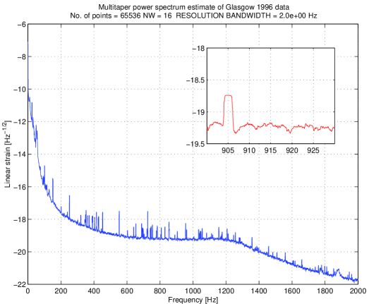
Figure 1: An estimate of two-sided spectral density of 1996 Glasgow data. The spectral feature shown in the insert is due to harmonics of the mains frequency.

The flat part corresponds to linear one-sided spectral density of around $10^{-19}$Hz^-1/2.

4 Data preparation

We have divided the data into blocks of $2^{8}$ points. We have singled out blocks of ’bad’ data by the following criterion. We have selected those blocks in which the maximum of the absolute values of the data in the block exceeded 8.5 Volts. We have then defined the window function $W_{n}$, $1\leq n\leq N$ as $0$ for each $n$ such that data sample $x_{n}$ is in the selected block of ’bad’ data and $1$ otherwise. We have also normalized the data set as follows. In each block of data we have subtracted from every point the block mean and divided by the block standard deviation. We have then multiplied the resulting sequence by the window function $W_{n}$. A similar procedure was applied in an analysis of 100 hours Garching data by Niebauer et al. [6]. Dividing the data by the block mean improves the signal-to-noise ratio (SNR) because periods of low noise make the highest contributions to overall SNR. Also the normalization reduces the slow variation of the mean and the variance of the noise thus removing some non-stationarity from the data.

5 Results of the tests for periodicity

We have calculated DFT of the whole data set (using the FFT algorithm) and we have analysed the periodogram for periodicities in the frequency range from around 450Hz to 1250Hz i.e. around $4\times 10^{6}$ Fourier bins altogether. We have divided DFT into blocks of length $R=2^{7}$ bins. We have chosen a very high significance level $\alpha$ of $10^{-6}$. We have applied a test based on the statistics $g_{A}$ in the following way: we have calculated the threshold form the Eq. (9) for $\alpha=10^{-6}$ and we have registered all the values of the normalized periodoram $g_{k}$ that crossed this threshold. The test yielded 14 significant events. The first 6 of them are shown in Figure 2.

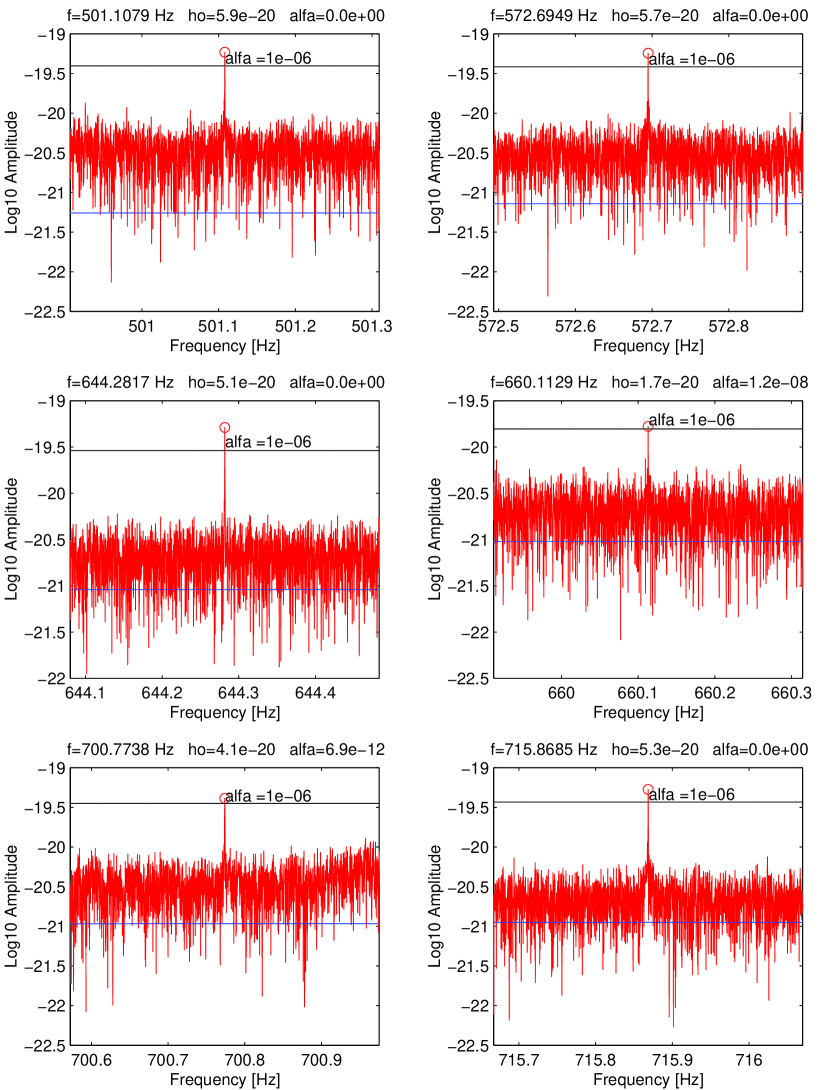
Figure 2: Narrow spectral features in the 1996 Glasgow data.

They were all narrow lines, 1 to 2 bins wide. We have also found that all these lines were harmonics of the following set of frequencies: $h_{1}=60.0103$Hz, $h_{2}=70.0774$Hz, $h_{3}=71.5869$Hz. On top of each frame in Figure 1 we have given the frequency $f$ of the detected spectral feature, the dimensionless amplitude $h_{o}$, the significance level $\alpha$ of the event calculated from Eq. (9) ($\alpha=0$ means that it is smaller than machine accuracy $\sim 2.2\times 10^{-16}$). If the spectral feature corresponds to a monochromatic signal form outside the detector then $h_{o}$ is the maximum-likelihood estimator of its amplitude. The upper line is the threshold corresponding to $10^{-6}$ significance level. The lower line is what we call ”pulsar line”. For the detector located in Glasgow it corresponds to the maximum amplitude of the gravitational wave of a pulsar at twice the pulsar spin frequency assuming ellipticity of $10^{-4}$, distance 40pc from the Earth, and moment of inertia of $10^{45}$gcm² w.r.t. the rotation axis. We consider this as the strongest pulsar signal possible with our current understanding of pulsar distribution in the galaxy and their physics. The results of Siegel’s test revealed 27 events: 7 more harmonics of the frequencies given above. One harmonic of frequency $h_{4}=72.8174$Hz (only one more harmonic of that frequency was found for much lower significance level of $5\times 10^{-2}$ with $g_{A}$ test), 2 narrow features riding on top of wide spectral features of bandwidth $~{}0.1$Hz, and three narrow, 1 bin wide lines of frequencies 510.4761Hz, 511.1870Hz, and 1210.5961Hz that could not be related to any harmonics. The amplitudes of the last three features were $35,30,26$ times above the pulsar line respectively. Two of the frequencies found by Jones [1] where 8th and 11th harmonics of the frequency $h_{1}$ given above, the third one $f_{G3}=675.0879$Hz was none of the frequencies reported above. Nevertheless we confirmed its existence in the data with a very low significance $\alpha=0.44$.

Comparision of the results of the two tests shows that the test based on the statistics $T_{A}$ is considerably more powerful in detecting periodicities in the spectrum than the test based on the statistics $g_{A}$. We have repeated the above analysis for various length of the data blocks and another criterion of tagging the bad data based on the magnitude of the variance in the block and also for various length $R$ of DFT blocks and the results of the above analyis have not changed substancially.

6 Conclusions

Our conclusion is that none of the spectral features detected by us could be confused with pulsar signals. Firstly we would not expect a gravitational wave from a pulsar to show in the Fourier domain as a series of harmonics. We can expect significant power around once and twice the pulsar spin frequency with harmonics of a much smaller amplitude. Secondly the amplitudes of all the spectral features including narrow single frequencies are much higher than for any possible gravitaional wave from a pulsar. Finally we point out that given only a finite number of samples of the data and no further information it is impossible to distinguish strict periodic components from peaks of arbitrary small width in the continuous spectrum [7]. The spectral lines that we detected are due to a periodic deterministic signal in the data if we know that the maximum width of the spectral features in the continuous part of the spectrum is greater than $R$ Fourier bins.

- [1] Jones G. S. 1996, Internal and informal report concerning Fourier analysis of data produced by the Glasgow laser interferometer in March 1996.
- [2] Fisher R. A., 1929, Proc. Royal Soc. Lond., Series A, 125, 54.
- [3] Siegel A. F., 1980, J. of Am. Stat. Association, 75, 345.
- [4] Percival D. B. and Walden A. T., Spectral analysis for physical applications, Cambridge University Press, Cambridge 1993, p.222.
- [5] Siegel A. F., 1979, Biometrika, 66, 381.
- [6] Niebauer T. M. et al., Phys. Rev. D 47, 3106 (1993).
- [7] Priestley M. B., Spectral analysis and time series, Academic Press 1981, p.619.