Gravitational-wave versus binary-pulsar
tests of strong-field gravity

Abstract

Binary systems comprising at least one neutron star contain strong gravitational field regions and thereby provide a testing ground for strong-field gravity. Two types of data can be used to test the law of gravity in compact binaries: binary pulsar observations, or forthcoming gravitational-wave observations of inspiralling binaries. We compare the probing power of these two types of observations within a generic two-parameter family of tensor-scalar gravitational theories. Our analysis generalizes previous work (by us) on binary-pulsar tests by using a sample of realistic equations of state for nuclear matter (instead of a polytrope), and goes beyond a previous study (by C.M. Will) of gravitational-wave tests by considering more general tensor-scalar theories than the one-parameter Jordan-Fierz-Brans-Dicke one. Finite-size effects in tensor-scalar gravity are also discussed.

I Introduction

The detection of gravitational waves by kilometric-size laser-interferometer systems such as LIGO in the US and VIRGO in Europe will initiate a new era in astronomy. One of the most promising sources of gravitational waves is the inspiralling compact binary, a binary system made of neutron stars or black holes whose orbit decays under gravitational radiation reaction. The observation of these systems will provide important astrophysical information, e.g. masses of neutron stars, and direct distance measurements up to hundreds of Mpc [2]. It is also said that detecting gravitational waves from inspiralling binaries should provide rich tests of the law of relativistic gravity in situations comprising strong-field regions (like near a neutron star or a black hole). However, present binary-pulsar experiments already provide us with deep and accurate tests of strong-field gravity [3, 4, 5]. It is therefore interesting to compare and contrast the probing power of present (and foreseeable) pulsar tests with that of future gravity-wave observations.

A convenient quantitative way of doing this comparison is to work within a multi-parameter family of physically motivated (and physically consistent) theories of gravity which differ from Einstein’s theory in their radiative and strong-field predictions. The most natural framework of this type is the general class of tensor-scalar theories in which gravity is mediated both by a tensor field $g_{\mu\nu}^{*}$ (“Einstein metric”) and by a scalar field $\varphi$. These theories contain one arbitrary “coupling function” $A(\varphi)$ defining the conformal factor relating the pure spin-2 Einstein metric $g_{\mu\nu}^{*}$ to the “physical metric” $\widetilde{g}_{\mu\nu}=A^{2}(\varphi)\,g_{\mu\nu}^{*}$ measured by laboratory clocks and rods. The usual Jordan-Fierz-Brans-Dicke theory [6, 7, 8] is the one parameter class of theories defined by a coupling function $A(\varphi)=\exp(\alpha_{0}\,\varphi)$. [The coupling strength $\alpha_{0}$ is related to the often used parameter $\omega$ by $\alpha_{0}^{2}=(2\omega+3)^{-1}$.] Will [9] has studied the quantitative constraints on the coupling parameter $\alpha_{0}$ of Jordan-Fierz-Brans-Dicke theories that could be brought by gravitational-wave observations. His result is that in most cases the bounds coming from gravity-wave observations will be comparable to presently known bounds coming from solar-system experiments (namely, $\alpha_{0}^{2}<10^{-3}$). This result of Ref. [9] seems to suggest that gravitational-wave-based strong-field tests of gravity do not go really beyond the solar-system weak-field tests of gravity. We wish, however, to emphasize that this seemingly pessimistic conclusion is mainly due to having restricted one’s attention to the special, one-parameter Jordan-Fierz-Brans-Dicke theory. Indeed, in this theory the strength of the coupling of the scalar field $\varphi$ to matter is given by the constant quantity $\alpha_{0}$ independently of the state of condensation of the gravitational source. As a consequence, the predictions of the theory differ from those of Einstein’s theory by a fraction of order $\alpha_{0}^{2}$ in all situations: weak-field ones or strong-field ones, alike. By contrast, it has been emphasized in Refs. [10, 11] that the more generic tensor-scalar theories in which the strength of the coupling of $\varphi$ to matter, namely

$$\alpha(\varphi)\equiv\frac{\partial\ln A(\varphi)}{\partial\,\varphi}\,,$$ (1)

depended on the value of $\varphi$, allowed for the existence of genuine strong-field effects, by which the presence of a highly condensed source, such as a neutron star, could generate order-unity deviations from general relativity even if the weak-field limit of $\alpha(\varphi)$ is arbitrarily small. [More precisely, these non-perturbative strong-field effects take place when $\beta(\varphi)\equiv\partial\,\alpha(\varphi)/\partial\,\varphi$ is negative.] This led us to consider, instead of the Jordan-Fierz-Brans-Dicke model $A(\varphi)=\exp(\alpha_{0}\varphi)$, the class of theories defined by

$$A(\varphi)=\exp\left(\frac{1}{2}\,\beta_{0}\varphi^{2}\right)\,.$$ (2)

This class of theories contains two arbitrary (dimensionless) parameters: $\beta_{0}$ appearing in Eq. (2), and $\varphi_{0}$, the asymptotic value of $\varphi$ at spatial infinity. [By contrast, in Jordan-Fierz-Brans-Dicke theory, $\varphi_{0}$ has no observable effects.] Equivalently, the two parameters in these theories can be defined as being the strength of the linear coupling of $\varphi$ to matter in the weak-field limit $(\varphi\approx\varphi_{0})$,

$$\alpha_{0}=\alpha(\varphi_{0})=\frac{\partial\ln A(\varphi_{0})}{\partial\,\varphi_{0}}=\beta_{0}\varphi_{0}\,,$$ (3)

and the non-linear coupling parameter

$$\beta_{0}=\frac{\partial\,\alpha(\varphi_{0})}{\partial\,\varphi_{0}}=\frac{\partial^{2}\ln A(\varphi_{0})}{\partial\,\varphi_{0}^{2}}\,.$$ (4)

A convenient feature of the two-parameter family of theories (2) is that they have just the amount of generality needed both to parametrize the most general boost-invariant weak-field (“post-Newtonian”) deviations from Einstein’s theory, and to encompass nonperturbative strong-field effects. Indeed, on the one hand, the two theory-parameters $(\alpha_{0},\beta_{0})$ determine the two well-known Eddington-Nordtvedt-Will parameters,

$$\overline{\gamma}\equiv\gamma_{\rm Eddington}-1=-2\,\alpha_{0}^{2}/(1+\alpha_{0}^{2})\,,$$ (5)

$$\overline{\beta}\equiv\beta_{\rm Eddington}-1=\frac{1}{2}\,\beta_{0}\,\alpha_{0}^{2}/(1+\alpha_{0}^{2})^{2}\,,$$ (6)

which measure the most general, boost-invariant, deviations from general relativity at the first post-Newtonian level. (See [12, 13] for the generalization of the Eddington parameters to the second post-Newtonian level.) On the other hand, when $\beta_{0}\lesssim-4$ non-perturbative strong-field effects develop in the theories defined by Eq. (2).

All existing gravitational experiments can be interpreted as constraints on the two-dimensional space of theories defined by Eq. (2). In other words, we can work within the common $(\alpha_{0},\beta_{0})$ plane, and consider each gravitational experiment (be it of weak-field or strong-field nature) as defining a certain exclusion plot within that plane. In some recent work [11], we have constructed such exclusion plots, as defined by considering both solar-system experiments and binary-pulsar experiments. The present work will generalize these exclusion plots in several respects: (i) we shall plot the regions of the $(\alpha_{0},\beta_{0})$ plane probed by future gravitational-wave observations of neutron star–neutron star, and neutron star–black hole systems, (ii) we shall improve our previous study of the probing power of binary-pulsar experiments by considering a sample of realistic nuclear equations of states (instead of the polytropic one used by us before) and by using updated pulsar data, and (iii) we shall consider the individual constraints on $\alpha_{0}$ and $\beta_{0}$ brought by the main solar-system experiments (instead of using published combined limits on $\overline{\gamma}$ and $\overline{\beta}$).

This paper is organized as follows: In Sec. II we summarize our (numerical) approach to computing the various form factors that describe the coupling of the scalar field $\varphi$ to a neutron star. In Sec. III we generalize Ref. [9] in discussing how gravitational wave observations can give quantitative tests of tensor-scalar gravity. In Sec. IV we combine and compare gravitational-wave tests with binary-pulsar tests and solar-system ones. Our conclusions are presented in Sec. V, while an Appendix discusses finite-size effects in tensor-scalar gravity.

II Gravitational form factors of neutron stars described by realistic equations of state

The orbital dynamics of a binary system depends, besides the Einstein masses of the two objects $m_{A}$, $m_{B}$, on the effective coupling constants $\alpha_{A}$, $\alpha_{B}$, defined as

$$\alpha_{A}\equiv\frac{\partial\ln m_{A}}{\partial\,\varphi_{0}}\,,$$ (7)

as well as on their scalar-field derivatives

$$\beta_{A}\equiv\frac{\partial\,\alpha_{A}}{\partial\,\varphi_{0}}\,.$$ (8)

The derivatives in Eqs. (7), (8) are taken for fixed values of the baryonic mass $\overline{m}_{A}$. In the limit of negligible self-gravity $\alpha_{A}\rightarrow\alpha_{0}$ and $\beta_{A}\rightarrow\beta_{0}$, but it was shown in Refs. [10, 11] that (when $\beta_{0}$ is negative enough) the effective coupling constant $\alpha_{A}$ of a neutron star can reach values of order unity even if the weak-field coupling constant $\alpha_{0}$ is extremely small. By contrast, in Jordan-Fierz-Brans-Dicke theory $\alpha_{A}$ tends to zero with $\alpha_{0}$. Let us also note that for a black hole $\alpha_{A}=0$ because of the no-scalar-hair theorems.

In Ref. [12] it was shown that the parameters $m_{A}$, $m_{B}$, $\alpha_{A}$, $\alpha_{B}$, $\beta_{A}$, $\beta_{B}$ suffice to determine both the $(v/c)^{2}$-accurate conservative orbital dynamics (including periastron precession and other relativistic deformations of Keplerian motion) and the radiation reaction effects (monopolar, dipolar and quadrupolar effects linked to the combined emission of scalar and tensor waves). On the other hand, the relativistic timing of binary pulsar systems involves, besides the above effective coupling constants, a new parameter describing the possible field dependence of the (Einstein-frame) inertia moment $I_{A}$ of the pulsar [14, 11]. This new parameter, entering the timing formula, is of the form $K_{A}^{B}=k_{A}\,\alpha_{B}$ where

$$k_{A}=-\frac{\partial\ln I_{A}}{\partial\,\varphi_{0}}\,.$$ (9)

For a fixed value of the baryonic mass $\overline{m}_{A}$, the quantities $m_{A}$, $\alpha_{A}$, $\beta_{A}$ and $k_{A}$ depend on: (i) the value $\varphi_{0}$ of the scalar field at infinity and the theory of gravity used (hence a dependence on $\alpha_{0}$ and $\beta_{0}$ in our case), and (ii) the equation of state of nuclear matter used to describe the interior of the neutron star.

In this work, we shall consider, besides the simple polytropic equation of state that we used before,

$$\widetilde{\epsilon}=\widetilde{n}\,\widetilde{m}_{b}+\frac{K\,\widetilde{n}_{0}\,\widetilde{m}_{b}}{\Gamma-1}\ \left(\frac{\widetilde{n}}{\widetilde{n}_{0}}\right)^{\Gamma}\,,\ \widetilde{P}=K\,\widetilde{n}_{0}\,\widetilde{m}_{b}\,\left(\frac{\widetilde{n}}{\widetilde{n}_{0}}\right)^{\Gamma}\,,$$ (10)

$$\widetilde{m}_{b}=1.66\times 10^{-24}{\rm g}\ ,\ \widetilde{n}_{0}=0.1\,{\rm fm}^{-3}\ ,\ \Gamma=2.34\ ,\ K=0.0195\ ,$$ (11)

a sample of three (more or less) realistic equations of state. They describe the crust by the same equation of state (due to Baym et al. [15]) but differ in their descriptions of the core of the neutron star. One description (due to Pandharipande [16]) gives a rather soft equation of state, a second one (due to Wiringa et al. [17]) is of intermediate stiffness, while the third one (due to Haensel et al. [18]) corresponds to a somewhat stiff equation of state. This sample will allow us to see the effect of the softness of the equation of state.

We have discussed in detail in Ref. [11] the way to compute the effective coupling constants $m_{A}$, $\alpha_{A}$, $\beta_{A}$, $k_{A}$ in tensor-scalar gravity. We shall not repeat this material here. Let us only mention a modification that we brought to the procedure discussed in Ref. [11] for more convenience when dealing with equations of state given in tabular form. Starting from such tables, we first interpolate them to define the (proper) physical energy density $\widetilde{\epsilon}$ and the (proper) physical baryon number density $\widetilde{n}$ as functions of the physical pressure $\widetilde{p}$. [The tilde refers here to quantities expressed in “physical units”, i.e., with respect to the metric $\widetilde{g}_{\mu\nu}=A^{2}\,g_{\mu\nu}^{*}$.] Then, we transform the field equations by using the pressure $\widetilde{p}$ as a radial variable. More precisely, this means that we consider a set of 8 first-order differential equations for the variation with $\widetilde{p}$ of the variables $M$, $\nu$, $\varphi$, $\psi$, $\rho$, $\overline{M}$, $\omega$ and $\varpi$. The symbols $M,\ldots,\varpi$ have the same meaning as in Ref. [11]. In particular, $\rho$ is the Schwarzschild-like radial coordinate used in Eq. (3.1) of [11]. Note that the quantity $\alpha_{0}$ is constructed at the end of the numerical work from the asymptotic value of $\varphi$ by using $\alpha_{0}=\beta_{0}\,\varphi_{0}$, Eq. (3). The right-hand side of the equation giving $d\rho/d\widetilde{p}$ is the inverse of the right-hand side of Eq. (3.6e) of [11], while the right-hand sides of the 7 other equations is simply obtained [from $dQ/d\widetilde{p}\equiv(dQ/d\rho)/(d\widetilde{p}/d\rho)$] by dividing the right-hand sides of Eqs. (3.6a)–(3.6h) by the right-hand side of Eq. (3.6e). A bonus of this modified approach is that we can numerically integrate these differential equations on a known range: namely, we start integration at the center of the star with some given central value for $\widetilde{p}$, say $\widetilde{p}_{c}$, and we stop at $\widetilde{p}=0$ (surface of the star). The value of $\rho$ at the end of integration gives the radius $R$ of the star. We have discussed in Refs. [10, 11] how to obtain the quantities $\overline{m}_{A}$, $m_{A}$, $\alpha_{A}$, and $I_{A}$ from the other results of the integration.

Actually, having chosen some nuclear equation of state, the above numerical integration yields, for each value of $\beta_{0}$, and for each initial values $\widetilde{p}_{c}$ (central pressure) and $\varphi_{c}$ (central value of the scalar field), an output which consists of ($\overline{m}_{A}$, $m_{A}$, $\alpha_{A}$, $I_{A}$, $\varphi_{0}$), where $\varphi_{0}$ is the value of $\varphi$ at spatial infinity. [We keep only the “positively scalar-polarized” configurations with $\varphi_{0}\,\varphi_{c}>0$. Indeed, we have shown in [11] that the solutions with $\varphi_{0}\,\varphi_{c}<0$ are energetically disfavored.] Having constructed a sufficiently dense grid (in $(\widetilde{p}_{c},\varphi_{c})$ space) of such numerically integrated models, we can then compute $\beta_{A}$, Eq. (8), and $k_{A}$, Eq. (9), by numerically approximating the $\varphi_{0}$-derivatives (with fixed $\overline{m}_{A}$) by finite differences constructed from four neighboring grid points. The expression (7) for $\alpha_{A}$ is used as a test of our numerical accuracy (we appropriately densify our grid so as to ensure that Eq. (7) is satisfied to better than $5\%$). Using finally some interpolation, we end up by generating a huge, multi-entry table which is conveniently organized as giving, for a grid of values of $\alpha_{0}$ and $\beta_{0}$, numerical values of $(\overline{m}_{A},m_{A},\alpha_{A},\beta_{A},I_{A},k_{A})$. This is a numerical approximation to giving $m_{A}$, $\alpha_{A}$, $\beta_{A}$, $I_{A}$ and $k_{A}$ as functions of $\alpha_{0}$, $\beta_{0}$ and $\overline{m}_{A}$. We should also mention that we keep only stable models in our tables, i.e., we keep only configurations corresponding to masses increasing, when the central pressure increases, between (formally) zero and their first maximum (corresponding to the usual concept of the maximum mass of a neutron star, here quantitatively modified by scalar-field effects).

III Testing tensor-scalar gravity from gravitational-wave observations of inspiralling binaries

The gravitational wave signal from inspiralling binaries will be deeply buried in the broadband noise of interferometric detectors. To detect it, one will have to correlate the output of the detector with a “template wave form”, i.e., an hopefully faithful copy of the actual time evolution of the signal. As hundreds to tens of thousands of cycles may be usefully registered in the output of the detector, this method of matched filtering will allow one to dig deeply into the broadband noise, under the condition that the used template wave form be an accurate representation of the signal over that many cycles. This means that gravitational wave observations will be very sensitive to the evolution of the frequency and the phase of the wave.

In tensor-scalar gravity the evolution of the phase of the gravitational wave will be different from that in Einstein’s pure tensor gravity because this phase evolution is driven by radiation reaction, which is modified because the system can now loose energy to scalar waves, in addition to loosing energy to tensor waves. More precisely, the energy lost to scalar or tensor radiation at infinity now reads, with sufficient approximation,

$$\dot{E}={\dot{E}}_{\varphi}^{\rm monopole}+{\dot{E}}_{\varphi}^{\rm dipole}+{\dot{E}}_{\varphi}^{\rm quadrupole}+{\dot{E}}_{h}^{\rm quadrupole}\,,$$ (12)

where the subscript denotes the field being radiated, and where the superscript refers to the multipolar structure of the emitted radiation. The explicit expressions for the various energy losses have been derived for general tensor-(multi-)scalar gravity theories in Ref. [12] (see also [19]). As said above, they depend on the (Einstein) masses $m_{A}$, $m_{B}$ and on the effective scalar coupling parameters of the two stars, $\alpha_{A}$, $\alpha_{B}$, $\beta_{A}$, $\beta_{B}$. Denoting $M\equiv m_{A}+m_{B}$, $X_{A}\equiv m_{A}/M$, $X_{B}\equiv m_{B}/M=1-X_{A}$, $\nu\equiv X_{A}X_{B}$, and assuming that the orbit is circularized (eccentricity $e=0$), we find from Eq. (6.52) of Ref. [12] the following evolution law for the orbital frequency $n=2\pi/P_{\rm orbit}$

$$\frac{\dot{n}}{n^{2}}=\frac{\nu}{1+\alpha_{A}\alpha_{B}}\ \left[\frac{96}{5}\,\kappa\ \left(\frac{v}{c}\right)^{5}+(\alpha_{A}-\alpha_{B})^{2}\,\left(\frac{v}{c}\right)^{3}+O\left(\left(\frac{v}{c}\right)^{6}\right)\right]\,,$$ (13)

where

$$v\equiv[G_{*}(1+\alpha_{A}\alpha_{B})\,Mn]^{1/3}$$ (14)

(in which $G_{*}$ denotes the “bare” gravitational constant entering the action of the Einstein metric: $\int d^{4}x\,g_{*}^{1/2}\,R(g_{*})/16\pi\,G_{*}$), and

$$\kappa \equiv 1+\frac{1}{6}\,(\alpha_{A}X_{B}+\alpha_{B}X_{A})^{2}+\frac{1}{6}\,(\alpha_{A}-\alpha_{B})(\alpha_{A}X_{A}+\alpha_{B}X_{B})(X_{A}-X_{B})$$ (15)

$$+ \frac{5}{48}\,\frac{\alpha_{A}-\alpha_{B}}{1+\alpha_{A}\alpha_{B}}\ (\beta_{B}\alpha_{A}X_{A}-\beta_{A}\alpha_{B}X_{B})+d_{2}\,(\alpha_{A}-\alpha_{B})^{2}\,.$$ (16)

The term $(\alpha_{A}-\alpha_{B})^{2}\,(v/c)^{3}$ in Eq. (13) is associated to the emission of scalar dipolar waves [14, 20, 19, 21]. The first term (equal to one) in $\kappa$ comes from the emission of tensor quadrupolar waves, the second term is due to the emission of scalar quadrupolar waves, the remaining terms come from $O((v/c)^{5})$ contributions to the scalar dipolar waves [responsible for the $O((v/c)^{3})$ term in Eq. (13)]. The numerical coefficient $d_{2}$ has not been computed, but this is not important in the present context as it multiplies the same term $(\alpha_{A}-\alpha_{B})^{2}$ which will be more strongly constrained by the $O((v/c)^{3})$ dipolar radiation term in Eq. (13). [Let us note in passing that our parameter $\kappa$ differs by a certain factor from the one used by Will [9], namely, $\kappa_{\rm will}=(1+\alpha_{A}\alpha_{B})^{2}\,(1+\alpha_{0}^{2})^{-3}\,\kappa_{\rm here}$.]

The expression (13) is similar to the frequency evolution equations used by Will [9]. Our results are, however, more general because they apply in a generic tensor-gravity theory, while his were restricted to the Jordan-Fierz-Brans-Dicke case. On the other hand, starting from Eq. (13) we can follow his analysis in discussing the constraints that can be derived from (future) gravitational wave observations. Let us define a tensor-scalar “chirp mass” (in time units) by

$${\cal M}\equiv\frac{G_{*}}{c^{3}}\ (1+\alpha_{A}\alpha_{B})\,M\,\left(\frac{\nu\,\kappa}{1+\alpha_{A}\alpha_{B}}\right)^{3/5}\,,$$ (17)

and the corresponding adimensionalized orbital frequency

$$u\equiv{\cal M}\,n\,.$$ (18)

In terms of these variables, Eq. (13) reads

$${\cal M}\,\dot{u} = \frac{96}{5}\ u^{11/3}\biggl{\{}1+b\,\nu^{2/5}\,u^{-2/3}+O(b\,\nu^{-1/5}\,u^{1/3})$$ (21)

$$-\left(\frac{743}{336}+\frac{11}{4}\ \nu\right)\ \nu^{-2/5}\,u^{2/3}\,[1+O(\alpha^{2})]$$

$$+4\pi\,\nu^{-3/5}\,u\,[1+O(\alpha^{2})]+O(u^{4/3})\biggr{\}},$$

where we defined

$$b\equiv\frac{5}{96}\ \kappa^{-3/5}\,(1+\alpha_{A}\alpha_{B})^{-2/5}\,(\alpha_{A}-\alpha_{B})^{2}\,.$$ (22)

The zeroth-order term $\propto u^{11/3}$ in Eq. (21) represent the frequency evolution due to the emission of tensor quadrupolar waves. The other terms represent corrections to this zeroth-order result. The terms containing a factor $b$ or a symbolic factor $\alpha^{2}$ represent the effects of the radiation of scalar waves. The main term due to the radiation of scalar waves is the $b\,\nu^{2/5}\,u^{-2/3}$ term. It is important to note that this term (coming from dipolar waves) contains the large factor $u^{-2/3}\sim v^{-2}\gg 1$. This term is the main source of the constraints on tensor-scalar gravity coming from gravity-wave observations because it has a different dependence on $u$ than the usual general relativistic terms. Indeed, the usual general relativistic frequency evolution is given by the terms without $b$ or $\alpha^{2}$ factors, i.e., symbolically, ${\cal M}\,\dot{u}\sim u^{11/3}\,[1+u^{2/3}+u^{3/3}+u^{4/3}+\cdots]$.

Assuming that future gravity-wave observations from inspiralling binaries will be well matched by filters constructed from the standard general relativistic orbital phase evolution, we wish to quantify what constraints they could bring on the modifications to the frequency evolution equation (21) by the terms proportional to $b$ or $\alpha^{2}$. This problem has been tackled by Will [9] using a matched-filter analysis. His analysis can be applied to our case, if we follow his (plausible) assumption that the final bounds will restrict scalar-field effects to be more or less uniformly small compared to general relativistic ones. This means that the only essential scalar-field term that we should consider in Eq. (21) is the term $b\,\nu^{2/5}\,u^{-2/3}$. All the scalar-field effects that simply modify usual einsteinian effects can be neglected. Furthermore, this means also that we can approximate $\kappa$ by one, and the chirp mass (17) by its einsteinian limit $G_{*}\,c^{-3}\,M\,\nu^{3/5}$. Finally, we can translate Will’s final bound on the Jordan-Fierz-Brans-Dicke coupling parameter $\alpha_{0}^{2}$ (his Eq. (5)), in the following bound on $b$ or $(\alpha_{A}-\alpha_{B})^{2}$:

$$\frac{48}{5}\ b\approx\frac{1}{2}\,(\alpha_{A}-\alpha_{B})^{2}<1.46\times 10^{-5}\,\left(\frac{\cal M}{T_{\odot}}\right)^{7/3}\,\nu^{-2/5}\,\left(\frac{10}{S/N}\right)\,,$$ (23)

where $T_{\odot}=G_{*}\,m_{\odot}\,c^{-3}$ is the gravitational time associated to a solar mass. This bound can also be rewritten in terms of $M=m_{A}+m_{B}$ and $\nu=m_{A}\,m_{B}/(m_{A}+m_{B})^{2}$:

$$(\alpha_{A}-\alpha_{B})^{2}<2.92\times 10^{-5}\,\left(\frac{M}{m_{\odot}}\right)^{7/3}\,\nu\,\left(\frac{10}{S/N}\right)\,.$$ (24)

In Eqs. (23) and (24), $S/N$ denotes the signal-to-noise ratio (after applying a matched filter) of a LIGO/VIRGO-type detector. [The analysis of Ref. [9] assumes the noise spectral density of a LIGO “advanced detector”.]

We have focussed above on the indirect effect of scalar-wave emission on the phase evolution of tensor waves for the following reason. Relatively to the main tensor-quadrupolar contribution, this effect is of order $(\alpha_{A}-\alpha_{B})^{2}\,(c/v)^{2}\gg(\alpha_{A}-\alpha_{B})^{2}$. Moreover, because of possible nonperturbative scalar-field effects associated to the strong self-gravity of neutron stars $(\alpha_{A}-\alpha_{B})^{2}$ can reach values of order unity, even if the weak-field scalar coupling $\alpha_{0}\ll 1$. By contrast, the more direct effect of scalar-wave emission on the differential forces acting on any (local) detector of gravitational waves can be described by the transverse projection of the physical metric $\widetilde{g}_{\mu\nu}$

$$\widetilde{g}_{ij}^{T}=(A^{2}(\varphi_{0}+\phi)\,g_{ij}^{*})^{T}\approx h_{ij}^{*TT}+2\,\alpha_{0}\,\phi\,\delta_{ij}^{T}\,,$$ (25)

where $\delta_{ij}^{T}\equiv\delta_{ij}-n_{i}\,n_{j}$ is the projection of $\delta_{ij}$ transversally to the direction $n^{i}$ of propagation of the wave (see, e.g., [12]), and where we choose units such that $A(\varphi_{0})=1$. The main direct effect of scalar-wave emission, associated, to scalar dipolar emission, is then (see Eq. (6.33) of [12])

$$2\,\alpha_{0}\,\phi^{\rm dipole}\,\delta_{ij}^{T}=-\frac{2}{r}\ \alpha_{0}\,(\alpha_{A}-\alpha_{B})\ \frac{m_{A}m_{B}}{M}\ n_{i}(z_{A}^{i}-z_{B}^{i})\,.$$ (26)

Compared to the standard tensor-quadrupolar wave, this is of order $\alpha_{0}\,(\alpha_{A}-\alpha_{B})\ (c/v)^{2}$. Even when nonperturbative strong-field effects generate $\alpha_{A}-\alpha_{B}=O(1)$, we see that the direct effects of scalar-wave emission are down by a factor $\alpha_{0}\ll 1$ compared to the indirect ones. One therefore a priori expects that these direct effects will be less sensitive probes of strong-field deviations from general relativity than the indirect ones considered above. This qualitative-argument-based conclusion is confirmed by the results of Will (Sec. IV of [9]) who quantified the lower sensitivity of matched filtering to amplitudes, as compared to phases.

Let us also note that Refs. [10, 11] have emphasized that gravitational collapse and neutron-star binary coalescence (by contrast with inspiral) might exhibit observably significant direct and indirect scalar-wave effects due to the combined possibilities of strong-scalar-field effects and monopolar radiation. [However, the recent investigation of Ref. [22] suggests that these effects will be too small to be of observational interest.]

IV Combining gravity-wave, pulsar and solar-system tests

Thanks to our consideration of a two-dimensional “mini-space” of alternative gravity theories, we can combine various experimental tests of relativistic gravity, and compare their probing power. Indeed, each experimental constraint separates the $(\alpha_{0},\beta_{0})$ plane into two regions: an allowed one and an excluded one (at some fixed confidence level). We can therefore compare the probing power of various experimental tests by drawing a combined exclusion plot in the $(\alpha_{0},\beta_{0})$ plane.

We shall consider three solar-system tests of weak-field gravity. The measurement of the Shapiro time delay by the Viking mission [23] as well a some VLBI measurements [24, 25] yield the $1\sigma$ bound $|\overline{\gamma}|<2\times 10^{-3}$, which (in view of Eq. (5)) gives

$$\alpha_{0}^{2}<10^{-3}\quad(1\sigma)\,.$$ (27)

The measurement of the perihelion advance of Mercury [26] gives $\frac{1}{3}\ |2\,\overline{\gamma}-\overline{\beta}|<10^{-3}$ which, using Eqs. (5) and (6), translates into

$$\left|\alpha_{0}^{2}+\frac{1}{8}\ \beta_{0}\,\alpha_{0}^{2}\right|<7.5\times 10^{-4}\quad(1\sigma)\,.$$ (28)

Finally, the Lunar Laser Ranging experiment [27] yields $-1.7\times 10^{-3}<4\,\overline{\beta}-\overline{\gamma}<3\times 10^{-4}$ which translates into

$$-8.5\times 10^{-4}<\alpha_{0}^{2}+\beta_{0}\,\alpha_{0}^{2}<1.5\times 10^{-4}\quad(1\sigma)\,.$$ (29)

These three constraints, taken together, exclude the region above the solid line labeled “1PN” in Figs. 1–4. Concerning binary-pulsar experiments we shall take into account three of them.

The PSR 1913+16 experiment uses the values of three well-measured phenomenological timing observables (“post-Keplerian parameters” [5]) $\dot{\omega}^{\rm obs}$, $\gamma^{\rm obs}$ and $\dot{P}_{b}^{\rm obs}$. [We neglect the low-precision measurement of the post-Keplerian parameters $r$ and $s$.] Here $\dot{\omega}^{\rm obs}$ denotes the observed secular rate of advance of the periastron, $\gamma^{\rm obs}$ denotes the observed value of the “Einstein” time-dilation parameter (entering $\Delta_{E}=\gamma\sin u$ [5]), and $\dot{P}_{b}^{\rm obs}$ denotes the secular change of the orbital period. The values we shall take for these observed parameters are [28]

$$\dot{\omega}^{\rm obs} = 4.226\,621\,(11)^{\circ}\ {\rm yr}^{-1}\,,$$ (31)

$$\gamma^{\rm obs} = 4.295\,(2)\times 10^{-3}\ {\rm s}\,,$$ (32)

$$\dot{P}_{b}^{\rm obs}-\dot{P}_{b}^{\rm gal} = -2.4101(85)\times 10^{-12}\,,$$ (33)

where figures in parentheses represent (realistic) $1\sigma$ uncertainties in the last quoted digits. In Eq. (33), $\dot{P}_{b}^{\rm gal}$ represents the sum of various galactic effects which must be subtracted from $\dot{P}_{b}^{\rm obs}$ to be able to compare it to theoretical predictions [29]. [We will take into account below the small modifications brought to it by tensor-scalar gravity, Eq. (9.22) of [12].] We need also the values of the Keplerian parameters

$$P_{b} = 27\,906.980\,780\,4(6)\ {\rm s}\,,$$ (35)

$$e = 0.617\,130\,8(4)\,.$$ (36)

As explained in detail in Ref. [11] one converts the three phenomenological (theory-independent) measurements (IV) into constraints on alternative gravity theories by using the predictions that, say, tensor-scalar gravity make for $\dot{\omega}$, $\gamma$, $\dot{P}_{b}$ as functions of the two (a priori unknown) masses $m_{A}$, $m_{B}$ and of the parameters (here $\alpha_{0}$, $\beta_{0}$) defining each tensor-scalar theory. As already mentioned above, the dependence on the theory-parameters $\alpha_{0}$, $\beta_{0}$ goes through the dependence of the post-Keplerian parameters $\dot{\omega}$, $\gamma$ and $\dot{P}_{b}$ on the effective coupling constants $\alpha_{A}$, $\alpha_{B}$, $\beta_{A}$, $\beta_{B}$, $k_{A}$. The explicit expressions of $\dot{\omega}^{\rm theory}(m_{A},m_{B},\alpha_{A},\beta_{A},k_{A},\ldots)$, $\gamma^{\rm theory}(m_{A},m_{B},\alpha_{A},\beta_{A},k_{A},\ldots)$ and $\dot{P}_{b}^{\rm theory}(m_{A},m_{B},\alpha_{A},\beta_{A},k_{A},\ldots)$ have been written down in Refs. [12] and [11]. We shall not reproduce them here. Using these expressions, we then define a goodness-of-fit statistics by minimizing over the physically a priori undetermined masses:

$$\chi^{2}\,(p_{i}^{\rm obs};\alpha_{0},\beta_{0})={\rm min}_{m_{A},m_{B}}\,\chi^{2}\,(p_{i}^{\rm obs};m_{A},m_{B},\alpha_{A},\beta_{A},k_{A},\ldots)\,,$$ (37)

where, for the simultaneous measurement of any number of post-Keplerian parameters $p_{i}$, one would define

$$\chi^{2}\,(p_{i}^{\rm obs};m_{A},m_{B},\alpha_{A},\beta_{A},\ldots)\equiv\sum_{i}\left(\sigma_{p_{i}}^{\rm obs}\right)^{-2}\left(p_{i}^{\rm theory}(m_{A},m_{B},\alpha_{A},\beta_{A},\ldots)-p_{i}^{\rm obs}\right)^{2}\,.$$ (38)

Here, we neglect the correlations between the measurements of the various post-Keplerian parameters.

In principle, when considering one or more pulsar experiments simultaneously, one can associate a confidence level (in the bayesian sense) to any region ${\cal R}$ in the theory-plane by integrating over ${\cal R}$ the normalized a posteriori probability density

$$d\alpha_{0}\,d\beta_{0}\,\pi_{\rm post}(\alpha_{0},\beta_{0})=d\alpha_{0}\,d\beta_{0}\,N\,\pi_{\rm prior}(\alpha_{0},\beta_{0})\,W_{1}({\bf p}_{1}^{\rm obs}\mid\alpha_{0},\beta_{0})\,W_{2}({\bf p}_{2}^{\rm obs}\mid\alpha_{0},\beta_{0})\ldots$$ (39)

where the probability (density) $W_{1}$ to observe, in the first pulsar experiment, the multiplet ${\bf p}_{1}^{\rm obs}$ (e.g. $(\dot{\omega}^{\rm obs},\gamma^{\rm obs},\dot{P}_{b}^{\rm obs})$) of post-Keplerian parameters can be approximated by the Gaussian

$$W_{1}({\bf p}_{1}^{\rm obs}\mid\alpha_{0},\beta_{0})=\exp\left[-\frac{1}{2}\ \chi^{2}({\bf p}_{1}^{\rm obs};\alpha_{0},\beta_{0})\right]$$ (40)

with the definition (37) above. In Eq. (39), $N$ is a normalization constant (such that $\int\int d\alpha_{0}\,d\beta_{0}\,\pi_{\rm post}(\alpha_{0},\beta_{0})=1$) and $\pi_{\rm prior}(\alpha_{0},\beta_{0})$ is some a priori probability density for the values of the theory parameters. A common (and convenient) way of choosing some confidence regions ${\cal R}$ is to define them from the various $\chi^{2}$. One can consider either the overlap (assumed to exist) of the various individual $\chi^{2}$ contour levels $\chi^{2}({\bf p}_{1}^{\rm obs};\alpha_{0},\beta_{0})=k_{1}$, $\chi^{2}({\bf p}_{2}^{\rm obs};\alpha_{0},\beta_{0})=k_{2}$, etc., or the combined $\chi^{2}$ contour levels: $\chi_{\rm tot}^{2}(\alpha_{0},\beta_{0})=k_{\rm tot}$, with $\chi_{\rm tot}^{2}\equiv\sum_{a}\chi^{2}({\bf p}_{a}^{\rm obs};\alpha_{0},\beta_{0})$. To each choice of ${\cal R}$, we associate a bayesian probability (“probability of causes”; the causes being here the unknown theory parameters $\alpha_{0},\beta_{0}$) by integrating (39) over ${\cal R}$. Here, we shall not try to quantify confidence levels in this way. We shall content ourselves by plotting individual $\chi^{2}=1$ contours. If several independent so-defined pulsar contours overlap, it is clear that the overlap region will define a rather high confidence level region for the total experiment combining these independent pulsar measurements.

As discussed in Section II above, it is essential in this discussion to decide upon some equation of state for nuclear matter. Each choice of nuclear equation of state defines its own corresponding exclusion plot. For example, we expect soft equations of state (like Pandharipande’s) to yield stronger constraints on the theory parameters $(\alpha_{0},\beta_{0})$. Indeed, they lead to more highly condensed neutron star models, and thereby to generically higher values of the effective couplings $\alpha_{A}$, $\beta_{A}$, $k_{A}$ for given $(\alpha_{0},\beta_{0})$ [12]. We shall consider successively the following equations of state: (i) in Fig. 1 the polytrope (10)-(11) (as used in our previous work [11]), (ii) in Fig. 2 the (soft) Pandharipande equation of state, (iii) in Fig. 3 the (medium) Wiringa et al. equation of state, and (iv) in Fig. 4 the (stiff) Haensel et al. equation of state.

The PSR 1534+12 experiment consists mainly of the high-precision measurements of three post-Keplerian parameters (which have to deal with strong-field effects without mixing of radiative ones [4]): $\dot{\omega}^{\rm obs}$, $\gamma^{\rm obs}$ and $s^{\rm obs}$. Here $s^{\rm obs}$ denotes a phenomenological parameter measuring the shape of the gravitational time delay [30, 5]. The values we shall take for these three observable parameters are [31]

$$\dot{\omega}^{\rm obs} = 1.755\,76(4)\,{}^{\circ}\ {\rm yr}^{-1}\,,$$ (42)

$$\gamma^{\rm obs} = 2.066(10)\times 10^{-3}\ {\rm s}\,,$$ (43)

$$s^{\rm obs} = 0.982(7)\,.$$ (44)

We shall also take into account the lower-precision measurement of the range-of-time-delay parameter $r^{\rm obs}$

$$r^{\rm obs}=6.7(1.3)\times 10^{-6}\ {\rm s}\,,$$ (45)

and we shall need the Keplerian observables

$$P_{b} = 36\,351.702\,6587(35)\ {\rm s}\,,$$ (47)

$$e = 0.273\,677\,7(5)\,,$$ (48)

$$x = 3.729\,463(3)\ {\rm s}\,.$$ (49)

Reference [31] gives also the observed value of the radiative parameter $\dot{P}_{b}^{\rm obs}$. However, it underlines that the theoretical significance of this measurement is (at present) highly uncertain because of the lack of an independent, reliable measurement of the distance to PSR 1534+12. Indeed, as discussed in [29], several galactic effects have to be subtracted from $\dot{P}_{b}^{\rm obs}$ before equating it to the theoretical prediction $\dot{P}_{b}^{\rm theory}$. These corrections are relatively small and sufficiently well known in the case of PSR 1913+16, while they are relatively large and insufficiently known in the case of PSR 1534+12. Because of this insufficient knowledge of the theoretically relevant combination $\dot{P}_{b}^{\rm obs}-\dot{P}_{b}^{\rm gal}$, we shall not take into account this observable in our exclusion plots below. [An alternative choice would be to take it into account but to enlarge the errors induced by the uncertainty on the distance. In that case, we found that its main effect is to forbid the horn-shaped region at the top-left of Fig. 1, which is anyway already ruled out by solar-system experiments as well as other binary-pulsar tests.]

Finally, we follow Ref. [11] in taking also into account the data on PSR 0655+64. This binary pulsar is composed of a neutron star of mass $m_{A}\approx 1.4\,m_{\odot}$ and a white dwarf companion of mass $m_{B}\approx 0.8\,m_{\odot}$, moving around each other on a nearly circular orbit in a period of about one day. This dissymmetric system is, potentially, a strong emitter of scalar dipolar waves. Indeed, we saw above that dipolar radiation losses are proportional to $(\alpha_{A}-\alpha_{B})^{2}\,(v/c)^{3}$. Here $\alpha_{B}$ does not differ significantly from the weak-field coupling $\alpha_{0}$ because the self-gravity of a white dwarf is very small, while $\alpha_{A}$ can reach values of order unity. We refer to Ref. [11] for the discussion of the constraints obtainable from this system. The end result is that we get the following (conservative) $1\sigma$ constraint

$$[\alpha_{A}(m_{A})-\alpha_{0}]^{2}<3\times 10^{-4}\,.$$ (50)

We use the corresponding $\chi_{0655+64}^{2}=1$ level in our exclusion plots.

For all the equations of state that we consider, we see on the exclusion plots Fig. 1–4 that the most stringent constraints coming from pulsar experiments are obtained by combining the 1913+16 exclusion region for $\beta_{0}\lesssim+1$ with that from 0655+64 for $\beta_{0}\gtrsim+1$. The resulting theoretical bounds are somewhat less stringent (by a factor of a few) than solar-system bounds when $\beta_{0}\gtrsim\beta_{c}$, while for $\beta_{0}\lesssim\beta_{c}$ pulsar experiments essentially exclude an infinite domain of the $(\alpha_{0},\beta_{0})$ plane which remained allowed by solar-system experiments. Here, $\beta_{c}$ denotes the (negative) critical value of $\beta_{0}$ below which nonperturbative strong-field effects develop, thereby exhibiting the unique strong-field probing power of pulsar experiments. As we see on Figs. 1–4, the value of $\beta_{c}$ depends on the equation of state. In particular, a soft equation of state leads to highly condensed neutron star configurations and, thereby, develop nonperturbative effects earlier than stiff equations of state: in other words $-\beta_{c}^{\rm soft}<-\beta_{c}^{\rm stiff}$. This is visible on Fig. 2 (Pandharipande) where the pulsar bound is more stringent than the solar-system ones for $\beta_{0}\lesssim-1$, while for stiffer equation of state it becomes more stringent only when $\beta_{0}\lesssim-3$.

Finally, we have added, for comparison, the exclusion regions defined by the gravity-wave observation limit (24), assuming a signal-to-noise ratio $S/N=10$. In absence of gravity-wave observations telling us about the precise masses of real inspiralling binaries, we have considered two fiducial cases: (i) a two-neutron-star system with Einstein masses $m_{A}=1.441\,m_{\odot}$, $m_{B}=1.388\,m_{\odot}$ (as measured in PSR 1913+16 when interpreted in general relativity), and (ii) a neutron star–black hole system with $m_{A}=1.4\,m_{\odot}$, $m_{B}=10\,m_{\odot}$. In case (i) neither the precise numerical values of the masses nor the fact that we fix Einstein masses instead of baryonic masses is crucial. What is crucial in our definition of the fiducial case (i) is that we assume a fractional mass difference $\Delta m/m\approx\Delta\overline{m}/\overline{m}\approx 4\%$, as large as in PSR 1913+16. Indeed, the over important dipolar radiation is proportional to $[\alpha_{A}(m_{A})-\alpha_{B}(m_{B})]^{2}\propto(\Delta m/m)^{2}$ as $\Delta m/m\rightarrow 0$. In case (ii), the no-scalar-hair theorems guarantee that $\alpha_{B}=0$ for a black hole (see, e.g., [12]), so that neutron-star-black-hole systems are always good a priori probes of possible scalar dipolar radiation.

Because of the complexity of the numerical calculation of the strong-field form factors of neutron stars (see Sec. II above), we could compute more precisely the exclusion regions for the polytropic equation of state, Eqs. (10)-(11). Therefore, it is in Fig. 1 that one sees best the shape of the regions possibly excluded by future gravitational wave data. The fiducial case (i) (à la 1913+16) excludes an ellipsoidal bubble which touches the $\beta_{0}$ axis around $\beta_{0}\approx-5$, while the fiducial case (ii) (neutron star–black hole) excludes the region above the nearly straight line $\alpha_{0}-0.03\,\beta_{0}\approx 0.15$ represented in Fig. 1. The corresponding excluded regions for realistic equations of state can be recognized on Figs. 2–4 as deformations of the just described regions for the polytropic case. Note that the bubble excluded by 1913+16-like systems (i) is smaller when the EOS is softer, and that it even disappears for Pandharipande’s equation of state (Fig. 2). In that case, the detection of such a system by a gravitational-wave interferometer would not constrain at all the space of theories.

The value $S/N=10$ chosen for Figs. 1–4 corresponds to the conventional event rate of 3 binary-neutron-star coalescences per year in a radius of 200 Mpc, and to a probably smaller event rate for neutron-star-black-hole coalescences. However, as pointed out by Will [32], the event rate is only slightly relevant to our discussion since a single system can suffice to constrain the space of gravity theories. It is therefore interesting to consider also the lucky discovery of an exceptionally near system, with a signal-to-noise ratio as large as $S/N=100$. The corresponding exclusion plots are displayed in Fig. 5, for the same polytropic equation of state as in Fig. 1. The bubble excluded by the 1913+16-like system is much larger, but still not competitive with present binary-pulsar tests. Similarly, the neutron-star-black-hole system is more constraining than in Fig. 1, but the slope of the corresponding line is only reduced by a factor $\sim\sqrt{10}$, although the signal-to-noise ratio is 10 times larger. This is due to the fact that the dominant dipolar radiation is proportional to the square of $\alpha_{A}$. Therefore, the lucky discovery of a nearby neutron-star-black-hole system would be slightly more constraining than present binary-pulsar tests in the region $-3\lesssim\beta_{0}<0$, but not better than present solar-system experiments. Moreover, one must keep in mind that solar-system experiments will improve in the mean time. In particular, NASA’s Gravity Probe B mission (due for launch in 2000) is expected to improve the probing of $\alpha_{0}$ down to the level $\alpha_{0}\sim\sqrt{10^{-5}}\approx 3\times 10^{-3}$.

Since we are mentioning the possibility of lucky discoveries, like those of PSRs 1913+16 and 1534+12, let us also quote the constraints which could be achieved if a binary pulsar with a black-hole companion were discovered. In that case, the main dipolar radiation would be proportional to $\alpha_{A}^{2}$ (since $\alpha_{B}=0$ for a black hole), instead of the small factor $(\alpha_{A}-\alpha_{B})^{2}\propto(\Delta m/m)^{2}$ appearing for binary-neutron-star systems. The mass of the black hole is not a crucial parameter for this discussion (we take $m_{B}=10\,m_{\odot}$). Assuming an orbital period $P_{b}$ and a measurement accuracy for $\dot{P}_{b}$ similar to those of PSR 1913+16, one finds that the constraints on $\alpha_{0}$ would be tightened by a factor $\sim 80$, i.e., that the bold lines of Figs. 1–5 would cross the vertical axis around $\alpha_{0}\approx 0.05/80\approx 6\times 10^{-4}$. In terms of the Eddington parameter $\gamma_{\rm Edd}$, Eq. (5), this corresponds to a level $|\gamma_{\rm Edd}-1|\lesssim 10^{-6}$, which is about a thousand times tighter than present solar-system limits, and ten times better than the probing level expected from Gravity Probe B. This underlines that, in the future, binary-pulsar tests may become competitive with, or even supersede, solar-system experiments even in the region $\beta_{0}>-4$ of the theory plane.

V Conclusions

The main conclusion of the comparison carried out in Figs. 1–5 is that, in all cases, future LIGO/VIRGO observations of inspiralling compact binaries turn out not to be competitive with present binary-pulsar tests in their discriminating probing of the strong-field, and radiative, aspects of relativistic gravity. This conclusion may seem paradoxical. It should not be interpreted negatively against LIGO/VIRGO observations which, as shown in Figs. 1–5, will independently probe strong-field gravity and will exclude regions of parameter space allowed by solar-system experiments. Rather, it is simply a reminder that binary-pulsar experiments are superb tools for probing strong-field and radiative aspects of gravity. It is also somewhat a good news for gravitational wave data analysis (which promises to be already a very challenging task even if one a priori assumes the validity of general relativity; see, e.g., [33]). Indeed, our results Figs. 1–5 indicate that our present experimental knowledge of the law of relativistic gravity is sufficient to justify using general relativity as the standard theory of gravitational radiation.

Note that this conclusion explicitly refers to the quantitative probing of plausible deviations from general relativity. At the qualitative level, and also at the non-discriminating quantitative level, LIGO/VIRGO observations will bring invaluable advances in our experimental knowledge of relativistic gravity. First, they will provide the first direct observation of gravitational waves far in the wave zone (while binary pulsar experiments prove the reality of the propagation with finite velocity of the gravitational interaction in the near zone of a binary system). Second, they will (hopefully) lead to superb additional confirmations of general relativity through the observation of the wave forms emitted during the inspiral and coalescence of neutron stars or black holes; see, e.g., [2, 34].

Independently of the comparison between LIGO/VIRGO tests and binary-pulsar tests, the present paper has provided the first systematic study of the influence of the nuclear equation of state on the theoretical probing power of binary-pulsar tests. In particular, Fig. 2 shows that if the equation of state were as soft as predicted by the simple Pandharipande model, binary-pulsar tests quantitatively supersede solar-system ones in all the region $\beta_{0}\lesssim-1$ of parameter space. Even if we consider the less constraining stiff equations of states, the present work confirms the limit

$$\beta_{0}>-4.5$$ (51)

found (modulo $10\%$) in [11]. We recall that this limit can be interpreted as a limit on the ratio of the two weak-field post-Einstein parameters

$$\frac{\beta_{\rm Edd}-1}{\gamma_{\rm Edd}-1}\approx-\frac{1}{4}\,\beta_{0}<1.1\,.$$ (52)

Finally, we pointed out that the discovery of a binary pulsar with a black-hole companion has the potential of providing a superb new probe of relativistic gravity. The discriminating power of this probe might supersede all its present and foreseeable competitors in measuring $\alpha_{0}$ down to the level $\alpha_{0}^{2}<10^{-6}$.

A Finite-size effects in tensor-scalar gravity

In the text we have assumed that the leading modification, in tensor-scalar gravity, of the orbital motion of binary systems comes from the change in radiation reaction forces. In this appendix, we briefly discuss the modifications of the orbital motion caused by the finite extension of the bodies. Contrary to the pure spin 2 theory where such effects are very small (because they are suppressed in spherical bodies), the presence of a scalar field opens the possibility of couplings to the spherical inertia moment $\int d^{3}{\bf x}\,\rho({\bf x})\,{\bf x}^{2}$. In this appendix we use the general diagrammatic approach of Ref. [13] to confirm (and hopefully better understand) the results of Nordtvedt [35, 36, 37] based on some explicit calculations valid only for weakly-self-gravitating extended bodies. The final outcome is that finite-size effects can be neglected in a matched-filter analysis of inspiralling compact binaries.

Following the indications given in [13], we can formally, but very generally, take extension effects into account by considering that the effective action for each compact body is a functional of the fields $\varphi$ and $g^{*}_{\mu\nu}$ which can be expanded in terms of the values along some central worldline of their spacetime derivatives (derivative expansion). Namely, we take the following action for the extended body (labeled $E$)

$$S_{E}^{\rm extended}=-c\int m_{E}^{\rm eff}\,[\varphi,g_{\mu\nu}^{*}]\left(-g_{\mu\nu}^{*}(z_{E}^{\lambda})\,dz_{E}^{\mu}\,dz_{E}^{\nu}\right)^{1/2}\,,$$ (A1)

with

$$m_{E}^{\rm eff}\,[\varphi,g_{\mu\nu}^{*}]=m_{E}(\varphi(z))+I_{E}(\varphi)\,R^{*}+J_{E}(\varphi)\,u_{E}^{*\mu}\,u_{E}^{*\nu}\,R_{\mu\nu}^{*}+K_{E}(\varphi)\,\Box^{*}\,\varphi$$ (A2)

$$+L_{E}(\varphi)\,u_{E}^{*\mu}\,u_{E}^{*\nu}\,\nabla_{\mu}^{*}\,\partial_{\nu}\,\varphi+M_{E}(\varphi)\,u_{E}^{*\mu}\,u_{E}^{*\nu}\,\partial_{\mu}\,\varphi\,\partial_{\nu}\,\varphi+N_{E}(\varphi)\,g^{*\mu\nu}\,\partial_{\mu}\,\varphi\,\partial_{\nu}\,\varphi\,.$$ (A3)

This is the most general action, expanded up to two derivatives of the fields $\varphi$ and/or $g_{\mu\nu}^{*}$, for a body which is spherically symmetric and static when unperturbed. [Terms which are first order in derivatives are excluded by spherical symmetry or, for $H_{E}(\varphi)\,u_{E}^{*\mu}\,\partial_{\mu}\,\varphi$, by time-reversal symmetry.] This form, being generic, is valid for strongly self-gravitating bodies. In this case, the $\varphi$-dependent quantities $I_{E}$, $J_{E}$, $K_{E}$, $L_{E}$, $M_{E}$, $N_{E}$, define some “scalar form factors” of body $E$ which go beyond the basic effective coupling $\alpha_{E}(\varphi)=\partial\ln m_{E}(\varphi)/\partial\,\varphi$ associated with the point-like effective action $S_{E}^{\rm point}=-c\int m_{E}(\varphi)\,d\,s_{E}^{*}$. [For non-spherical and/or non-static bodies many other new scalar form factors could, in principle, appear.]

Most of the a priori independent-looking terms in Eq. (A3) can be easily shown either not to contribute at the (observationally most relevant) first post-Keplerian level [i.e., $O(v^{2}/c^{2})$ beyond the Keplerian orbital motion], or to be equivalent to other terms, modulo some redefinition of the dynamical variables. Let us first recall that any correction term, in a Lagrangian, which is proportional to the zeroth-order equations of motion can be redefined away by shifting some of the dynamical variables. Technically, $S_{0}[\psi]+\epsilon\,I(\psi)\,\delta S_{0}/\delta\psi=S_{0}[\psi^{\prime}]+O(\epsilon^{2})$ with $\psi^{\prime}=\psi+\epsilon\,I(\psi)$. In our case, the dynamical variables can be either $g_{\mu\nu}^{*}$, $\varphi$ or $z_{E}^{\mu}$. In all cases, the local redefinitions $\psi\rightarrow\psi^{\prime}$ have no effects on the observables at infinity (such as the periastron advance or the evolution of the orbital phase of an inspiralling binary). Using such local redefinitions of the dynamical observables (and formally neglecting singular self-action terms, i.e., $\delta$-function contributions to $m_{E}^{\rm eff}[\varphi]$), one easily checks the following simplifications: The $J_{E}(\varphi)$ contribution can be transformed (using the $g_{\mu\nu}^{*}$ field equations $R_{\mu\nu}^{*}=2\partial_{\mu}\,\varphi\,\partial_{\nu}\,\varphi+\delta$-functions and a local redefinition of $g_{\mu\nu}^{*}$ within body $E$) into the $M_{E}(\varphi)$ contribution. The $M_{E}(\varphi)$ term contributes only at the second post-Keplerian level $O(v^{4}/c^{4})$. The $K_{E}(\varphi)$ term can be eliminated by redefining $\varphi$ within body $E$. The $L_{E}(\varphi)$ term can be reabsorbed in the $N_{E}(\varphi)$ one by redefining the position $z_{E}^{\mu}$, and by neglecting second post-Keplerian (2PK) effects. Indeed, integrating by parts $-\int cds_{E}^{*}\,L_{E}(\varphi)\,u^{*\mu}\,u^{*\nu}\,\nabla_{\mu}^{*}\,\partial_{\nu}\,\varphi$ one finds an $M_{E}(\varphi)$-like term (contributing only at 2PK order) plus a term proportional to $u^{*\mu}\,\nabla_{\mu}^{*}\,u^{*}_{\nu}$, which is equal to $-\alpha_{E}(\delta_{\nu}^{\mu}+u^{*\mu}\,u_{\nu}^{*})\,\partial_{\mu}\,\varphi$ upon using the equations of motion. This shows that after the redefinition

$$z_{E}^{\mu}\rightarrow z_{E}^{\prime\mu}=z_{E}^{\mu}+\frac{L_{E}}{\widetilde{m}_{E}}\ \nabla^{*\mu}\varphi\,,$$ (A4)

the $L_{E}(\varphi)$ contribution is, modulo 2PK, equivalent to changing $N_{E}(\varphi)\rightarrow N^{\prime}_{E}(\varphi)=N_{E}+\alpha_{E}\,L_{E}$. Similarly, the $I_{E}$ term can be absorbed in the $N_{E}$ one by locally redefining $g_{\mu\nu}^{*}$. [In fact, if one fixes the harmonic gauge before making this redefinition of $g_{\mu\nu}^{*}$, one also needs a shift of the positions of the bodies $A\neq E$ to absorb $I_{E}$ into $N_{E}$, namely, $z_{A}^{i}\rightarrow z_{A}^{\prime i}=z_{A}^{i}+4G_{*}I_{E}(z_{A}^{i}-z_{E}^{i})/(r_{EA}^{3}c^{2})+O(1/c^{4})$.]

Finally, we end up (modulo 2PK) with a generic, simplified effective action containing only a $N_{E}$-type two derivative term:

$$S_{E}^{\rm new}=-c\int ds_{E}^{*}\,[m_{E}(\varphi)+N_{E}^{\rm new}(\varphi)\,g^{*\mu\nu}\,\partial_{\mu}\,\varphi\,\partial_{\nu}\,\varphi]\,,$$ (A5)

where

$$N_{E}^{\rm new}=N_{E}+\alpha_{E}\,L_{E}+2I_{E}\,.$$ (A6)

The conclusion is that, modulo $O(v^{4}/c^{4})$ terms and higher-order terms in the radius of the extended body $E$ (associated to higher-derivatives), there is only one relativistic form factor for, possibly compact, extended bodies in tensor-scalar gravity: $N_{E}^{\rm new}$. By dimensional analysis $[N_{E}^{\rm new}]=[{\rm mass}]\,[{\rm length}]^{2}$ and we therefore expects $N_{E}^{\rm new}$ to be, roughly, some spherical inertia moment. Using the diagrammatic method of Ref. [13], it is easy to compute the extra contribution to the $N$-body Lagrangian entailed by the presence of $N_{E}$:

$$\delta^{\rm extended}\,L_{N{\rm-body}}=-\sum_{A\neq E\neq B}\ \frac{G_{*}^{2}\,m_{A}\,m_{B}\,(\alpha_{A}\,N_{E}^{\rm new}\,\alpha_{B})\,{\bf n}_{EA}\cdot{\bf n}_{EB}}{r_{EA}^{2}\,r_{EB}^{2}\,c^{2}}\,,$$ (A7)

where ${\bf n}_{EA}\equiv({\bf z}_{E}-{\bf z}_{A})/r_{EA}$. Note that in a two-body system the summation will have two terms: one where $E=1$, $A=B=2$, and one where $E=2$, $A=B=1$. [We denote here for clarity the two bodies by the labels 1 and 2.]

The above considerations have the advantage of being valid even when discussing strongly self-gravitating extended bodies. In the case of a weakly self-gravitating extended body, Nordtvedt [37] has obtained an effective action, after some explicit calculations of the equations of motion, of the form

$$S_{E}=-c\int ds_{E}^{*}\,\left[m_{E}(\varphi)+\frac{1}{6}\ \widetilde{I}_{E}\,A^{2}(\varphi)\,\widetilde{u}^{\mu}\,\widetilde{u}^{\nu}\,\widetilde{R}_{\mu\nu}\right]\,,$$ (A8)

where $\widetilde{I}_{E}=\int d^{3}\widetilde{x}\,\widetilde{\rho}(\widetilde{x})\,\widetilde{\bf x}^{2}$ is the physical spherical inertia moment, and where we recall that the tilde refers to physical, Jordan-frame quantities: $\widetilde{g}_{\mu\nu}=A^{2}\,g_{\mu\nu}^{*}$, $\widetilde{R}_{\mu\nu}=R_{\mu\nu}[\widetilde{g}]$, $\widetilde{g}_{\mu\nu}\,\widetilde{u}^{\mu}\,\widetilde{u}^{\nu}=-1$. By expanding (A8) in terms of our generic expansion (A3) we find

$$I_{E}=0\ ,\ J_{E}=\frac{1}{6}\,\widetilde{I}_{E}\ ,\ K_{E}=\frac{\alpha_{0}}{6}\,\widetilde{I}_{E}\ ,\ L_{E}=-\frac{\alpha_{0}}{3}\,\widetilde{I}_{E}$$ (A9)

$$M_{E}=-\frac{1}{3}\,(\beta_{0}-\alpha_{0}^{2})\,\widetilde{I}_{E}\ ,\ N_{E}^{\rm old}=\frac{1}{6}\,(\beta_{0}+2\alpha_{0}^{2})\,\widetilde{I}_{E}\,.$$ (A10)

We conclude from Eq. (A6) that the only observable form factor from infinity is

$$N_{E}^{\rm new}=\frac{1}{6}\,\beta_{0}\,\widetilde{I}_{E}\,.$$ (A11)

In other words, after the shift $z_{E}^{\prime\mu}=z_{E}^{\mu}-\frac{1}{3}\,\alpha_{0}\,(\widetilde{I}_{E}/\widetilde{m}_{E})\,\nabla^{*\mu}\,\varphi$, the only new contribution to the $N$-body Lagrangian is Eq. (A7) with $N_{E}^{\rm new}$ given by (A11). When comparing with Nordtvedt’s results, note that he does not perform the simplifying shift that we are advocating so that he ends up with a more complicated-looking $N$-body Lagrangian containing a contribution like (A7) but with $N_{E}^{\rm old}=\frac{1}{6}\,(\beta_{0}+2\alpha_{0}^{2})\,\widetilde{I}_{E}$, plus two other sums which are simply obtainable by applying the inverse shift ${\bf z}_{E}^{\rm Nordtvedt}={\bf z}_{E}^{\rm us}+\frac{1}{3}\,\alpha_{0}\,(\widetilde{I}_{E}/\widetilde{m}_{E})\,\mbox{\boldmath$\nabla$}\varphi$, with $\varphi=\varphi_{0}-\sum_{A}G_{*}\,m_{A}\,\alpha_{A}/r_{A}\,c^{2}$, to the unperturbed Lagrangian $L_{0}({\bf z}_{A},{\bf v}_{A})=\sum_{A}\frac{1}{2}\,m_{A}\,{\bf v}_{A}^{2}+\sum_{A\neq B}\frac{1}{2}\,G_{*}\,m_{A}\,m_{B}\,(1+\alpha_{A}\,\alpha_{B})/r_{AB}$. [Here, both ${\bf v}_{A}=\dot{\bf z}_{A}$ and $r_{AB}=|{\bf z}_{A}-{\bf z}_{B}|$ get modified by the shift.] Finally, we find that in a binary system the finite-size effects cause the appearance of the additional interaction energy terms

$$\delta^{\rm extended}\,E_{\rm int}=+\frac{G_{*}^{2}\,m_{A}\,m_{B}}{r_{AB}^{4}\,c^{2}}\ (\alpha_{A}^{2}\,N_{B}^{\rm new}+\alpha_{B}^{2}\,N_{A}^{\rm new})\,.$$ (A12)

For compact bodies (radius $R_{A}$ comparable to $G_{*}\,m_{A}/c^{2}$) we expect that $N_{A}^{\rm new}\sim\beta_{A}\,m_{A}(G_{*}\,m_{A}/c^{2})^{2}$, so that the new interaction energy (A12) will be of the form

$$\delta^{\rm extended}\,E_{\rm int}\sim(C_{B}\,\beta_{B}\,\alpha_{A}^{2}+C_{A}\,\beta_{A}\,\alpha_{B}^{2})\,E_{\rm 3PK}^{\rm GR}\,,$$ (A13)

where $E_{\rm 3PK}^{\rm GR}$ denotes the general relativistic third post-Keplerian $(O(v^{6}/c^{6}))$ contribution to the interaction energy, and where $C_{A}$ and $C_{B}$ are numerical coefficients which are roughly of order unity. The 3PK energy $E_{\rm 3PK}^{\rm GR}\sim G_{*}\,m_{A}\,m_{B}/r_{AB}\times(G_{*}\,m_{A}/c^{2}\,r_{AB})^{3}$ depends on the distance $r_{AB}$ in the same way as $\delta^{\rm extended}\,E_{\rm int}$.

The conclusion is that scalar-mediated finite-size effects can be neglected in a matched-filter analysis of the phase evolution of inspiralling binaries, because they only modify by a factor $\sim 1+C\,\beta\,\alpha^{2}$ (which tends to 1 as $\alpha^{2}\rightarrow 0$) terms already present in the general relativistic phase evolution. As discussed for similar fractional corrections in Section III, they can be neglected compared to the non-general-relativistic scalar dipolar contribution to the phase evolution.

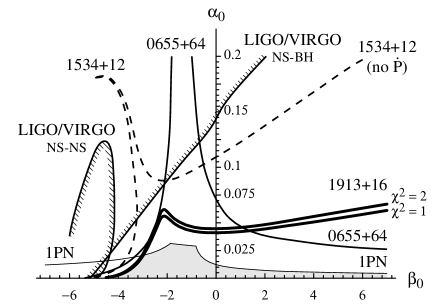
FIG. 1.: Region of the $(\alpha_{0},\beta_{0})$ theory plane allowed by solar-system tests, binary-pulsar experiments, and future gravity-wave detections, in the case where nuclear matter is described by the polytrope (10)-(11). In view of the reflection symmetry $\alpha_{0}\rightarrow-\alpha_{0}$, we plot only the upper half plane. The region allowed by solar-system tests is below the thin line labeled “1PN”. The PSR 0655+64 data constrain the values of $\alpha_{0}$ and $\beta_{0}$ to be between the two solid lines. The regions allowed by the PSR 1913+16 and PSR 1534+12 tests lie respectively to the right of the bold line and of the the dashed line. The horn-shaped region at the top-left of the dashed line is removed if the observable $\dot{P}_{b}^{\rm obs}$ is taken into account for PSR 1534+12. Each of these curves determines the level $\chi^{2}=1$ for the corresponding test. We have also plotted the level $\chi^{2}=2$ for PSR 1913+16 to underline that the precise value of $\chi^{2}$ is not very significant in the region where binary-pulsar experiments are more constraining than solar-system tests ($\beta_{0}\,{\lesssim}-3$). The regions excluded by the gravity-wave observation limit (24), with a signal-to-noise ratio $S/N=10$, lie on the hatched sides of the curves labeled “LIGO/VIRGO”. The case of a $1.4\,m_{\odot}$-neutron-star and a $10\,m_{\odot}$-black-hole binary system is labeled “NS-BH”, whereas the case of a 1913+16-like binary-neutron-star system is labeled “NS-NS”. The region simultaneously allowed by all the tests is shaded.

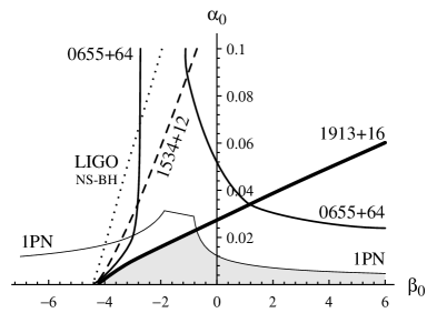
FIG. 2.: Same plot as Fig. 1 in the case of a soft equation of state (Pandharipande). The region possibly excluded by the LIGO/VIRGO detection of a ($1.4\,m_{\odot}$) neutron star–($10\,m_{\odot}$) black hole system lies above the dotted line. The bubble-like region at the left of Fig. 1 (binary-neutron-star system detected by LIGO/VIRGO) does not exist in the case of this soft equation of state.

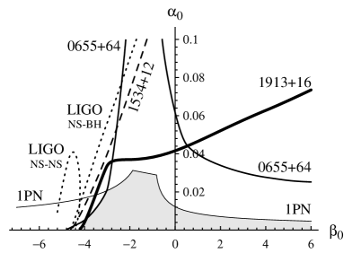
FIG. 3.: Same plot as Fig. 2 for a medium equation of state (Wiringa et al.). Dotted lines indicate the regions excluded by future gravitational-wave observations, respectively inside the bubble for the NS-NS case, and above the straight line for the NS-BH case.

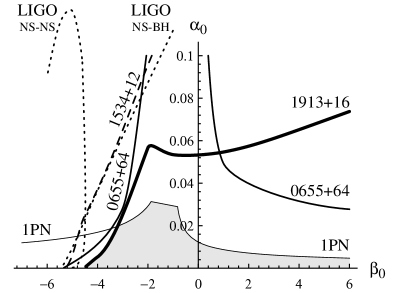
FIG. 4.: Same plot as Fig. 3 for a stiff equation of state (Haensel et al.). Note that the bubble excluded by the detection of a binary-neutron-star system by LIGO/VIRGO is much larger when the equation of state is stiff.

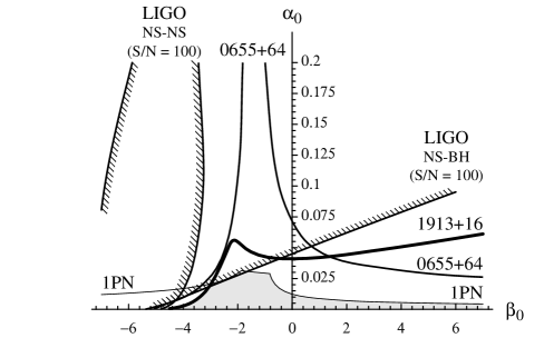
FIG. 5.: Same plot as Fig. 1, assuming the same polytropic equation of state, but a signal-to-noise ratio $S/N=100$ for the LIGO (hatched) curves. For clarity, the dashed line corresponding to the PSR 1534+12 test has been suppressed.

REFERENCES

- [1] Unité Propre de Recherche 7061.
- [2] K.S. Thorne, eprint gr-qc/9706079, to appear in Black Holes and Relativistic Stars, Proceedings of a Conference in Memory of S. Chandrasekhar, edited by R.M. Wald (University of Chicago Press, Chicago).
- [3] J.H. Taylor, Rev. Mod. Phys. 66, 711 (1994).
- [4] J.H. Taylor, A. Wolszczan, T. Damour, and J.M. Weisberg, Nature (London) 355, 132 (1992).
- [5] T. Damour and J.H. Taylor, Phys. Rev. D 45, 1840 (1992).
- [6] P. Jordan, Nature (London) 164, 637 (1949); Schwerkraft und Weltall (Vieweg, Braunschweig, 1955); Z. Phys. 157, 112 (1959).
- [7] M. Fierz, Helv. Phys. Acta 29, 128 (1956).
- [8] C. Brans and R.H. Dicke, Phys. Rev. 124, 925 (1961).
- [9] C.M. Will, Phys. Rev. D 50, 6058 (1994).
- [10] T. Damour and G. Esposito-Farèse, Phys. Rev. Lett. 70, 2220 (1993).
- [11] T. Damour and G. Esposito-Farèse, Phys. Rev. D 54, 1474 (1996).
- [12] T. Damour and G. Esposito-Farèse, Class. Quantum Grav. 9, 2093 (1992).
- [13] T. Damour and G. Esposito-Farèse, Phys. Rev. D 53, 5541 (1996).
- [14] D.M. Eardley, Astrophys. J. 196, L59 (1975).
- [15] G. Baym, C. Pethick, and P. Sutherland, Astrophys. J. 170, 299 (1971).
- [16] V.R. Pandharipande, Nucl. Phys. A174, 641 (1971).
- [17] R.B. Wiringa, V. Fiks, and A. Fabrocini, Phys. Rev. C 38, 1010 (1988).
- [18] P. Haensel, M. Kutschera, and M. Proszynski, Astron. Astrophys. 102, 299 (1980).
- [19] C.M. Will, Theory and Experiment in Gravitational Physics (Cambridge University Press, Cambridge, England, 1993).
- [20] C.M. Will, Astrophys. J. 214, 826 (1977).
- [21] C.M. Will and H.W. Zaglauer, Astrophys. J. 346, 366 (1989).
- [22] J. Novak, eprint gr-qc/9707041, to appear in Phys. Rev. D.
- [23] R.D. Reasenberg et al., Astrophys. J. Lett. 234, L219 (1979).
- [24] D.S. Robertson, W.E. Carter, and W.H. Dillinger, Nature (London) 349, 768 (1991).
- [25] D.E. Lebach et al., Phys. Rev. Lett. 75, 1439 (1995).
- [26] I.I. Shapiro, in General Relativity and Gravitation 1989, edited by N. Ashby, D.F. Bartlett, and W. Wyss (Cambridge University Press, Cambridge, England, 1990), p. 313.
- [27] J.G. Williams, X.X. Newhall, and J.O. Dickey, Phys. Rev. D 53, 6730 (1996).
- [28] J.H. Taylor, Class. Quantum Grav. 10, S167 (1993).
- [29] T. Damour and J.H. Taylor, Astrophys. J. 366, 501 (1991).
- [30] T. Damour and N. Deruelle, Ann. Inst. H. Poincaré 44, 263 (1986).
- [31] I.H. Stairs et al., eprint astro-ph/9712296.
- [32] C.M. Will, private communication.
- [33] T. Damour, B.R. Iyer, and B.S. Sathyaprakash, Phys. Rev. D 57, 885 (1998).
- [34] L. Blanchet and B.S. Sathyaprakash, Class. Quantum Grav. 11, 2807 (1994); Phys. Rev. Lett. 74, 1067 (1995).
- [35] K. Nordtvedt, Astrophys. J. 264, 620 (1983).
- [36] K. Nordtvedt, Phys. Rev. D 43, 3131 (1991).
- [37] K. Nordtvedt, Phys. Rev. D 49, 5165 (1994).