Abstract

We present an autonomous phase-plane describing the evolution of Friedmann-Robertson-Walker models containing a perfect fluid (with barotropic index $\gamma$) in Brans-Dicke gravity (with Brans-Dicke parameter $\omega$). We find self-similar fixed points corresponding to Nariai’s power-law solutions for spatially flat models and curvature-scaling solutions for curved models. At infinite values of the phase-plane variables we recover O’Hanlon and Tupper’s vacuum solutions for spatially flat models and the Milne universe for negative spatial curvature. We find conditions for the existence and stability of these critical points and describe the qualitative evolution in all regions of the $(\omega,\gamma)$ parameter space for $0\leq\gamma\leq 2$ and $\omega>-3/2$. We show that the condition for inflation in Brans-Dicke gravity is always stronger than the general relativistic condition, $\gamma<2/3$.

1 Introduction

One of the simplest extensions to the Einstein-Hilbert action of general relativity is the introduction of a scalar field non-minimally coupled to the metric tensor [1]. The simplest scalar-tensor theory is that proposed by Brans and Dicke [2] where the gravity theory contains only one dimensionless parameter, $\omega$, and the effective gravitational constant is inversely proportional to the scalar field, $\Phi$. This theory yields the correct Newtonian weak-field limit, but solar system measurements of post-Newtonian corrections require $\omega>500$ [3]. In the limit $\omega\to\infty$ the field $\Phi$ becomes fixed and we recover Einstein gravity. This has led to more general scalar-tensor gravity theories [4, 5, 6] being considered with a self-interaction potential $V(\Phi)$ [7, 8] or a variable $\omega(\Phi)$ [9] in order to fix $\Phi$ by the present day.

The fact that such scalar-tensor gravity theories are a generic prediction of low-energy effective supergravity theories from string theory [10] or other higher-dimensional gravity theories [11] has led to considerable interest in cosmological models of the very early universe derived from Brans-Dicke gravity. The time-dependent gravitational constant introduces a new degree of freedom into cosmological models which has led different authors to propose extended inflation [12], pre big bang [13] and gravity-driven inflation models [14] of the early universe, as well as modifications to conventional inflation [15] or nucleosynthesis models [16].

In this paper we will investigate the qualitative evolution of Friedmann-Robertson-Walker (FRW) models containing a barotropic perfect fluid in Brans-Dicke gravity. In Section 3 we review the asymptotic behaviour for spatially flat FRW models and the general solution which can be given in parametric form for barotropic fluids [17, 18]. Analytical solutions for spatially curved models are only possible in a limited number of special cases such as for radiation [19, 20, 21, 14] or stiff fluid [20, 22] and other methods are required to study the general behaviour. In Section 4 the field equations describing the cosmological evolution of the Brans-Dicke field and scale factor are reduced to two coupled autonomous first-order equations. A phase-plane analysis [23] is then used to solve qualitatively for the cosmological evolution [24, 25]. We present for the first time a compactified phase-plane which represents both late and early time behaviour for flat $(k=0)$ and curved $(k\neq 0)$ FRW models. In section 5 the cosmological evolution is described qualitatively for all regions of parameter space $(\gamma,\omega)$, where the Brans-Dicke parameter $\omega>-3/2$ and the barotropic index of the fluid $0\leq\gamma\leq 2$. In Section 6 we consider whether it is possible to construct cosmological solutions with infinite proper lifetimes in some parameter regimes. Our results are summarised in Section 7.

2 Equations of motion

We will consider here the simplest scalar-tensor theory as originally proposed by Brans and Dicke, where the gravity theory is characterised by a single dimensionless parameter $\omega$, representing the strength of coupling between the scalar field and the metric. The equations of motion are derived by extremizing the action

$$S=\frac{1}{16\pi}\int d^{4}x\,\sqrt{-g}\,\left[\Phi R-\frac{\omega}{\Phi}g^{\mu\nu}\Phi_{,\mu}\Phi_{,\nu}+16\pi{\cal L}_{\rm matter}\right]\ .$$ (2.1)

Homogeneous and isotropic cosmologies can be described by the Friedmann-Robertson-Walker (FRW) metric,

$$ds^{2}=-dt^{2}+a(t)^{2}\left[\frac{dr^{2}}{1-kr^{2}}+r^{2}(d\theta^{2}+\sin^{2}\theta d\phi^{2})\right]\ ,$$ (2.2)

The evolution equations for the scale factor, $a(t)$, and the Brans–Dicke field, $\Phi(t)$, can then be written as

$${\ddot{a}\over a} = -{8\pi\over 3\Phi}\left({3\omega P+(\omega+3)\rho\over 2\omega+3}\right)+{\dot{a}\over a}{\dot{\Phi}\over\Phi}-{\omega\over 3}\left({\dot{\Phi}\over\Phi}\right)^{2}\ ,$$ (2.3)

$$\ddot{\Phi} = -3\frac{\dot{a}}{a}\dot{\Phi}+{8\pi(\rho-3P)\over 2\omega+3}\ ,$$ (2.4)

where a dot denotes differentiation with respect to cosmic time, $t$. Matter with density $\rho$ and pressure $P$ obeys the continuity equation

$$\dot{\rho}=-3\frac{\dot{a}}{a}(\rho+P)\ .$$ (2.5)

These evolution equations possess a first-integral which corresponds to the generalised Friedmann constraint for the Hubble expansion, $H\equiv\dot{a}/a$,

$$H^{2}=\frac{8\pi\rho}{3\Phi}-H\frac{\dot{\Phi}}{\Phi}+\frac{\omega}{6}\left(\frac{\dot{\Phi}}{\Phi}\right)^{2}-\frac{k}{a^{2}}\ .$$ (2.6)

Considerable insight can be gained into the dynamical evolution of these models by working with the conformally rescaled Einstein metric [26, 27]

$$\tilde{g}_{\mu\nu}=(G_{N}\Phi)g_{\mu\nu}\ ,$$ (2.7)

where $G_{N}$ is Newton’s constant which remains fixed in the Einstein frame. The rescaled scale factor becomes $\tilde{a}=(G_{N}\Phi)^{1/2}a$ and the cosmic time

$$\tilde{t}=\int(G_{N}\Phi)^{1/2}dt\ .$$ (2.8)

The constraint equation (2.6) then can be written as the familiar Friedmann constraint

$$\tilde{H}^{2}={8\pi G_{N}\over 3}\left(\tilde{\rho}+\hat{\rho}\right)-{k\over\tilde{a}^{2}}\ ,$$ (2.9)

where $\tilde{H}$ is the Hubble expansion in the Einstein frame, $\tilde{\rho}=\rho/(G_{N}\Phi)^{2}$, and

$$\hat{\rho}={2\omega+3\over 12}\left({1\over\Phi}{d\Phi\over d\tilde{t}}\right)^{2}\ ,$$ (2.10)

is the effective energy density of the Brans-Dicke field in the Einstein frame. This has an effective pressure $\hat{P}=\hat{\rho}$, but is non-minimally coupled to the barotropic fluid. Note however that from the Friedmann constraint equation (2.9) we can immediately deduce that only closed models ($k>0$) have a turning point $\tilde{H}=0$ in the Einstein frame for $2\omega+3>0$. Theories with $2\omega+3<0$ have a negative energy density in the Einstein frame, implying that the Minkowski vacuum spacetime is unstable, and so we shall not consider such models here.

An equation of state for matter, $P(\rho)$, is needed in order to solve these equations of motion. We restrict our analysis to barotropic fluids where the pressure is simply proportional to the density, $P=(\gamma-1)\rho$, which includes the case of pressureless dust ($\gamma=1$), radiation ($\gamma=4/3$) or a false vacuum energy density ($\gamma=0$). The continuity equation (2.5) can then be integrated to give the matter density as a function of the cosmological scale factor $a(t)$

$$\rho=\frac{\Gamma}{a^{3\gamma}}\\$$ (2.11)

and this allows us to eliminate both $\rho$ and $P$ from the remaining equations of motion.

General analytic solutions for scalar–tensor cosmologies exist for only a limited number of special cases. For example we can solve analytically for a general FRW models in vacuum ($\rho=0$) [28, 21] or when the matter is radiation ($P=\rho/3$) [19, 20, 21, 14] or a stiff fluid ($P=\rho$) [20, 22] when the system reduces to perfect fluids in the Einstein frame. In Brans–Dicke gravity the general analytic solution for other cases can only be given in parametric form for spatially flat models ($k=0$) and we shall review these results briefly before going on to study the evolution of the more general FRW models.

3 Spatially-flat solutions

Brans and Dicke’s original motivation was to produce a model where the effective gravitational constant decreases ($\Phi$ increases) as the density of the universe decreases. In their original paper [2], Brans and Dicke gave a power-law solution for the evolution of a spatially flat FRW model filled with pressureless dust

$$a\propto|t-t_{*}|^{p}\ ,\qquad\Phi\propto|t-t_{*}|^{q}\ ,$$ (3.1)

where $p=(2\omega+2)/(3\omega+4)$, and $q=2/(3\omega+4)$. This was generalised to arbitrary barotropic equation of state by Nariai who found [29]

$$p = \frac{2\omega(2-\gamma)+2}{3\omega\gamma(2-\gamma)+4}$$ (3.2)

$$q = \frac{2(4-3\gamma)}{3\omega\gamma(2-\gamma)+4}\ .$$ (3.3)

This yields the general relativistic solution, $a\propto t^{2/3\gamma}$ with $\Phi$ constant, in the limit $\omega\to\infty$.

However Nariai’s power-law solution is in fact only a particular solution. The general solution can be given analytically in terms of a rescaled time coordinate

$$dT\equiv\frac{dt}{a^{3(\gamma-1)}}$$ (3.4)

Then the scale factor and Brans–Dicke field evolve as [17, 18]

$$a = a_{0}(T-T_{-})^{n_{\mp}}(T-T_{+})^{n_{\pm}}\ ,$$ (3.5)

$$\Phi = \Phi_{0}(T-T_{-})^{m_{\mp}}(T-T_{+})^{m_{\pm}}\ ,$$ (3.6)

where

$$n_{\pm} = \frac{\omega}{3\left(1+\omega(2-\gamma)\mp\sqrt{1+2\omega/3}\right)}$$ (3.7)

$$m_{\pm} = \frac{1\pm\sqrt{1+2\omega/3}}{1+\omega(2-\gamma)\mp\sqrt{1+2\omega/3}}$$ (3.8)

The solution where $T_{+}=T_{-}$ reduces to Nariai’s power–law solution given by Eqs. (3.1–3.3), and this is clearly the attractor solution when $T\to\infty$. However, substituting a solution of the form given in Eq. (3.1) into the definition of the time coordinate $T$ in Eq. (3.4) we can see that $t\to\infty$ at a finite value of $T$ if $3(\gamma-1)p>1$. Thus Nariai’s solutions are not necessarily the attractor solutions at late cosmic times. This case needs to be studied more carefully to determine the attractor behaviour which we shall do in the phase-plane analysis that follows.

As $T$ approaches $T_{+}$ or $T_{-}$ the general evolution (for $T_{-}\neq T_{+}$) approaches the vacuum solutions ($\rho=0$) first presented by O’Hanlon and Tupper [28], which are also power-law solutions of the form given in Eq. (3.1) with

$$p_{\pm}={n_{\pm}\over 1+3(\gamma-1)n_{\pm}} = \frac{\omega+1\pm\sqrt{1+2\omega/3}}{4+3\omega}\ ,$$

$$q_{\pm}={m_{\pm}\over 1+3(\gamma-1)n_{\pm}} = \frac{-2}{1\pm 3\sqrt{1+2\omega/3}}\ .$$ (3.9)

Nariai’s solution is sometimes described as the matter-dominated ($T\to\infty$) solution as opposed to the vacuum-dominated ($T\to T_{\pm}$) solution. The vacuum-dominated evolution has two solutions which have been termed fast or slow [17] depending on the early time behaviour of the scalar field $\Phi$. The slow solution corresponds to $(p_{-},q_{-})$ defined above where at early times the scalar field $\Phi$ is increasing (and $G\to 0$) as cosmic time increases for $\omega>-4/3$. The fast solution is defined by $(p_{+},q_{+})$, with $\Phi$ decreasing (and $G\to\infty$) as $t$ increases for $\omega>-4/3$.

The Brans-Dicke effective action Eq. (2.1) reduces to the truncated string effective action in the absence of matter ($\rho=0$) when the coupling constant $\omega=-1$ [10]. For comparison with the string literature we will define,

$$\phi\equiv-\ln\Phi\ ,\qquad\alpha=\ln a\ .$$ (3.10)

It can be shown that the spatially flat FRW solutions are related by a “scale-factor duality” [30]

$$\alpha\rightarrow-\alpha\ ,\qquad\phi\rightarrow\phi-6\alpha\ .$$ (3.11)

This scale–factor duality relates expanding cosmologies to contracting ones. Lidsey [31] has shown that this duality can be extended to all values of $\omega$ for vacuum solutions in Brans–Dicke gravity,

$$\alpha \rightarrow \left(\frac{2+3\omega}{4+3\omega}\right)\alpha-2\left(\frac{1+\omega}{4+3\omega}\right)\phi$$

$$\phi \rightarrow -\left(\frac{6}{4+3\omega}\right)\alpha-\left(\frac{2+3\omega}{4+3\omega}\right)\phi\ ,$$ (3.12)

which reduces to Eq. (3.11) when $\omega=-1$. Thus the fast and slow solutions defined above are interchanged under the above duality transform

$$(p_{\pm},q_{\pm})\rightarrow(p_{\mp},q_{\mp})$$ (3.13)

4 Autonomous phase-plane

In the absence of analytic solutions for general FRW models we seek a qualitative description of the evolution of the cosmological scale factor and scalar field with respect to time [23, 24, 25]. We shall now show that we can reduce the equations of motion (2.3) and (2.4) to a two-dimensional autonomous phase-plane whose qualitative evolution can be described for any values of the Brans-Dicke parameter $\omega$ or barotropic index $\gamma$.

The trace of the energy-momentum tensor for matter acts like a potential gradient term driving the scalar field $\Phi$ in Eq. (2.4) and so, in analogy with the phase-plane analysis of self-interacting scalar fields in general relativity [33, 34, 35], we can absorb the matter terms on the right-hand side of both the field equations (2.3) and (2.4) by introducing a new time coordinate, $\tau$, such that

$$d\tau\equiv\sqrt{\frac{8\pi\rho}{(3+2\omega)\Phi}}\,dt$$ (4.1)

We introduce two new variables [24]

$$x \equiv \frac{1}{2}\frac{\Phi^{\prime}}{\Phi}\ ,$$ (4.2)

$$y \equiv \frac{a^{\prime}}{a}\ .$$ (4.3)

Substitution of these variables in the equations of motion (2.4) and (2.3) yields

$$x^{\prime} = -x^{2}-\frac{3(2-\gamma)}{2}xy+\frac{4-3\gamma}{2}\ ,$$ (4.4)

$$y^{\prime} = {-2(1-3\alpha^{2})\over 3\alpha^{2}}x^{2}+3xy+{3\gamma-2\over 2}y^{2}-{3(4-3\gamma)\alpha^{2}+3\gamma-2\over 6\alpha^{2}}\ ,$$ (4.5)

where for convenience we have defined

$$\alpha^{2}\equiv\frac{1}{2\omega+3}\ .$$ (4.6)

We will consider only models for which $\omega>-3/2$ and thus $\alpha^{2}>0$.

The constraint equation (2.6) becomes

$$(x+y)^{2}=\frac{1}{3\alpha^{2}}\left(1+x^{2}\right)-\frac{3\Phi k}{8\pi\rho\alpha^{2}a^{2}}$$ (4.7)

By comparison with the Einstein frame constraint equation (2.9) we see that $(x+y)$ describes the expansion in the Einstein frame, and $x^{2}$ the effective energy density of the Brans-Dicke field relative to the barotropic fluid. The spatially flat ($k=0$) models lie on a separatrix in the phase–plane:

$$x+y=\pm\,{\sqrt{1+x^{2}}\over\sqrt{3}\alpha}\ .$$ (4.8)

Note that in order for $k=0$ models to have a turning point in the scale factor ($y=0$) we require $3\alpha^{2}>1$, i.e., $\omega<0$.

The equations (4.4) and (4.5) are two first-order differential equations forming a autonomous dynamical system in $x$ and $y$. The simultaneous solution of such equations defines a set of trajectories in the $(x,y)$ plane. The graphical representation of these equations form a system of ‘integral curves’ where

$$\frac{dy}{dx}=\frac{Q(x,y)}{P(x,y)}$$ (4.9)

where the functions $P(x,y)$ and $Q(x,y)$ are defined by the right hand sides of (4.4) and (4.5) respectively. This allows the qualitative evolution of the variables $x$ and $y$ to be determined.

4.1 Critical points in the finite plane

The key aspect of a phase plane analysis is to determine the critical points $(x_{i},y_{i})$ for the system. These are fixed points where the time derivatives of the variables vanish,

$$x^{\prime}=0\ ,\qquad y^{\prime}=0\ .$$ (4.10)

For an integral curve approaching such a point, the critical point represents the asymptotic behaviour either at the start or the end of the evolution.

Firstly we seek critical points at finite values $(x_{i},y_{i})$ in the phase plane. Requiring $x^{\prime}=0$ implies

$$x_{i}^{2}\left(1+\frac{3(2-\gamma)}{2}\frac{y_{i}}{x_{i}}\right)=\frac{4-3\gamma}{2}\ .$$ (4.11)

Requiring in addition that $y^{\prime}=0$ generates two possible solutions:

$$(a) \hskip 14.45377pt3\alpha^{2}(x_{a}+y_{a})^{2}=(1+x_{a}^{2})$$ (4.12)

$${\rm or}\hskip 14.45377pt (b) \hskip 14.45377pt(2-3\gamma)y_{b}=2x_{b}$$ (4.13)

Simultaneous solution of Eq. (4.11) with either Eq. (4.12) or (4.13) gives expressions for the critical points:

$$(x_{a\pm},y_{a\pm}) = \pm\left(\frac{\alpha(4-3\gamma)}{\sqrt{3(2-\gamma)^{2}-\alpha^{2}(4-3\gamma)^{2}}},\frac{(2-\gamma)-\alpha^{2}(4-3\gamma)}{\alpha\sqrt{3(2-\gamma)^{2}-\alpha^{2}(4-3\gamma)^{2}}}\right)$$ (4.14)

$$(x_{b\pm},y_{b\pm}) = \pm\left(\frac{\sqrt{2-3\gamma}}{2},\frac{1}{\sqrt{2-3\gamma}}\right)$$ (4.15)

Note that from the definitions of the variables $x$ and $y$ in Eqs. (4.2) and (4.3) the phase plane is symmetric under the $180^{\circ}$ rotation $x\to-x$ and $y\to-y$ plus time reversal $\tau\to-\tau$. Thus for every critical point $x_{i+},y_{i+}$ we have a critical point $x_{i-},y_{i-}$. In the remainder of this section we shall refer only to the critical points with $x_{i+}+y_{i+}>0$ which correspond to expanding solutions in the Einstein frame. It should be taken as read that there will be a point with $x_{i-}=-x_{i+}$ and $y_{i-}=-y_{i+}$ which corresponds to the time reversed solutions.

Also from the definitions of $x$ and $y$ we see that the fixed points $(x_{i},y_{i})$ correspond to solutions for $\Phi\propto e^{2x_{i}\tau}$ and $a\propto e^{y_{i}\tau}$ with respect to the time coordinate $\tau$. The evolution at the fixed points is self-similar as the nature of the solutions is unaffected by a rescaling $\tau\to\tau+\Delta\tau$. Integration of Eq. (4.1) then gives

$$t-t_{*}={2\over 2x_{i}+3\gamma y_{i}}\sqrt{{(3+2\omega)\Phi_{0}a_{0}^{3\gamma}\over 8\pi\Gamma}}\ e^{(2x_{i}+3\gamma y_{i})\tau/2}\ .$$ (4.16)

This ensures that we can only have cosmic time $t\to\infty$ at critical points in the finite phase-plane when $\tau\to\infty$ (for $2x_{i}+3\gamma y_{i}\geq 0$) and $t\to-\infty$ when $\tau\to-\infty$ (for $2x_{i}+3\gamma y_{i}\leq 0$). Critical points thus correspond to power-law solutions with respect to cosmic time for the scale factor $a$ and scalar field $\Phi$ of the form given in Eq. (3.1) where

$$p_{i}=\frac{2y_{i}}{2x_{i}+3\gamma y_{i}}\ ,\qquad q_{i}=\frac{4x_{i}}{2x_{i}+3\gamma y_{i}}\ .$$ (4.17)

4.1.1 Point $(a)$

Critical point $(x_{a},y_{a})$ always lies on the $k=0$ separatrix, as can be seen by comparing Eqs. (4.12) and (4.7). Substituting Eq. (4.14) into Eq. (4.17) we see that point $(a)$ corresponds to Nariai’s power-law solution for $k=0$ given in Eqs. (3.2) and (3.3).

From Eq. (4.14) we see that point $(a)$ exists for $\alpha<\sqrt{3}(2-\gamma)/|4-3\gamma|$ which implies that $\omega>\omega_{a}(\gamma)$, where we define

$$\omega_{a}(\gamma)\equiv\frac{-(10-6\gamma)}{3(2-\gamma)^{2}}$$ (4.18)

It can be seen that $(x_{a},y_{a})$ tends to infinity as $\omega\to\omega_{a}(\gamma)$. In the limit $\gamma\to 2$ we require $\omega\to\infty$ for $(x_{a},y_{a})$ to exist at finite values in the phase plane. On the other hand, as $\omega\to-3/2$ we find that $\gamma$ is restricted to $4/3$ for point $(a)$ to exist, as shown in Figure 1.

For point $(a)$ to correspond to an expanding universe, $\dot{a}>0$, requires $y_{a}>0$ and hence, from Eq. (4.14), $\omega>\omega_{+}(\gamma)$, where we define

$$\omega_{+}(\gamma)\equiv{-1\over 2-\gamma}$$ (4.19)

Note also that we have $t\to+\infty$ as $\tau\to+\infty$ in Eq. (4.16) at point $(a)$ only if $\omega\geq\omega_{-}(\gamma)$, where we define

$$\omega_{-}(\gamma)\equiv\frac{-4}{3\gamma(2-\gamma)}\ .$$ (4.20)

Conversely we have $t\to-\infty$ as $\tau\to-\infty$ only for $\omega\leq\omega_{-}(\gamma)$. In the particular case $\omega=\omega_{-}(\gamma)$, point $(a)$ corresponds to a non-singular exponential expansion, $a\propto\exp(Ht)$, where the Hubble rate, $H$, is a constant.

Nariai’s solution corresponds to an accelerated scale factor, $\ddot{a}>0$, if $p>1$ or $p<0$. For $p<0$ this requires $\omega_{-}(\gamma)<\omega<\omega_{+}(\gamma)$, in which case point $(a)$ corresponds to a contracting universe. For $p>1$ we require $\omega>\omega_{*}(\gamma)$ when $\gamma<2/3$, where we define

$$\omega_{*}(\gamma)\equiv\frac{2}{(2-\gamma)(2-3\gamma)}\ ,$$ (4.21)

or $\omega_{a}(\gamma)<\omega\leq\omega_{-}(\gamma)$ when $1<\gamma<4/3$. But only in the former case do we have $\omega>\omega_{+}(\gamma)$ and hence an accelerated, expanding universe. See Figure 1.

For the particular case $\gamma=0$ (corresponding to a false vacuum energy density), point $(a)$ corresponds to

$$a\propto t^{\omega+1/2}\ ,\qquad\Phi\propto t^{2}$$ (4.22)

which is the basis of models of extended inflation solution [12] when $\omega>\omega_{*}(0)=1/2$.

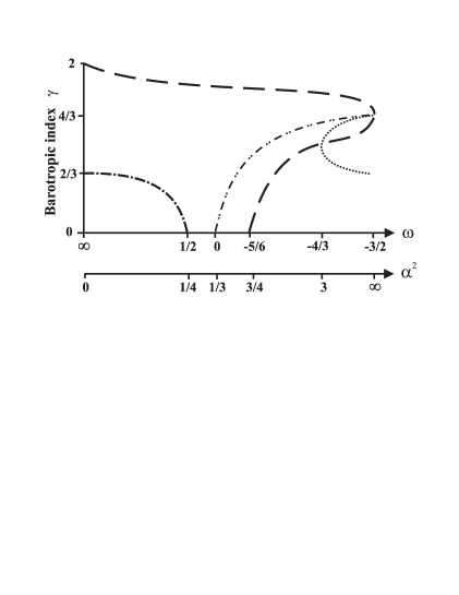
Figure 1: Lines dividing regions in parameter space with different cosmological behaviour at critical point $(a)$. The dashed line represents $\omega_{a}(\gamma)$, defined in Eq. (4.18). The single dot-dashed line represents $\omega_{*}(\gamma)$, defined in Eq. (4.21). The double dot-dashed line represents $\omega_{+}(\gamma)$, defined in Eq. (4.19). The dotted line represents $\omega_{-}(\gamma)$ as defined in Eq. (4.20).

4.1.2 Point $(b)$

Critical point $(x_{b},y_{b})$ is a novel power-law solution which corresponds to a curvature scaling solution [24, 25]. Substituting Eq. (4.15) into Eqs. (3.1) and (4.17) we find

$$a\propto t\ ,\qquad\Phi\propto t^{2-3/\gamma}\ .$$ (4.23)

Thus we have $\Phi\propto a^{2-3\gamma}$ and so the gravitational effect of the matter remains proportional to that of the curvature in the constraint Eq. (2.6)

$$\left(\frac{\dot{a}}{a}\right)^{2}\propto\frac{\rho}{\Phi}\propto\frac{k}{a^{2}}\ .$$ (4.24)

The universe expands with $a\propto t$, as it would in general relativity when $\gamma=2/3$ and $\rho\propto 1/a^{2}$ in general relativity. In Brans-Dicke theory this solution exists for all $\gamma\leq 2/3$. Point $(b)$ maybe described as marginal inflation, in the sense that although the spatial curvature does not vanish with respect to the gravitational energy density in the constraint equation (2.6), it does not grow either, and remains proportional to the gravitational energy density as $t\to\infty$.

Point $(b)$ exists for $\gamma\leq 2/3$, irrespective of the value of $\omega$ [24, 25]. In the limit $\gamma\to 2/3$ we have $x_{b}\to 0$ and $y_{b}\to\infty$. Note that $2x_{b}+3\gamma y_{b}>0$ whenever point $(b)$ exists and thus we have $t\to+\infty$ as $\tau\to+\infty$ in Eq. (4.16).

When $\omega=\omega_{*}(\gamma)$, defined in Eq. (4.21), point $b$ lies on the $k=0$ separatrix and the critical points $(x_{a},y_{a})$ and $(x_{b},y_{b})$ coincide. When $\omega>\omega_{*}$ point $(b)$ lies in the $k>0$ region, while for $\omega<\omega_{*}$ it lies in the $k<0$ region.

4.2 Stability of critical points in the finite plane

To determine the stability of these solutions we expand about the critical points

$$x = x_{i}+u$$ (4.25)

$$y = y_{i}+v$$ (4.26)

and substitute into the equations of motion for $x$ and $y$, Eqs. (4.4) and (4.5). This yields, to first-order in $u$ and $v$,

$$u^{\prime} = -\left(2x_{i}+{3(2-\gamma)\over 2}y_{i}\right)u-\left({3(2-\gamma)\over 2}x_{i}\right)v$$ (4.27)

$$v^{\prime} = \left(-{4(1-3\alpha^{2})\over 3\alpha^{2}}x_{i}+3y_{i}\right)u+\left(3x_{i}+(3\gamma-2)y_{i}\right)v$$ (4.28)

We seek the two eigenvalues $\lambda_{\pm}$ such that

$$u^{\prime}=\lambda_{\pm}u\ ,\qquad v^{\prime}=\lambda_{\pm}v\ ,$$ (4.29)

for the eigenmodes $u=K_{\pm}v$, where $K_{\pm}$ are constants. The eigenvalues are given by the roots of the quadratic

$$\lambda^{2}+B\lambda+C=0$$ (4.30)

where

$$B_{i} \equiv {10-9\gamma\over 2}y_{i}-x_{i}$$ (4.31)

$$C_{i} \equiv -6\left({(1-3\alpha^{2})(2-\gamma)\over 3\alpha^{2}}+1\right)x_{i}^{2}-2(3\gamma-2)x_{i}y_{i}-{3(2-\gamma)(3\gamma-2)\over 2}y_{i}^{2}$$ (4.32)

The critical point is a stable, attractor solution if the real part of both the eigenvalues is negative (i.e., $B_{i}>0$ and $C_{i}>0$). Linear perturbations about such points are then exponentially damped. A saddle point in the phase–plane has one negative and one positive real root ($C_{i}<0$). An unstable node has eigenvalues with positive real parts ($B_{i}<0$ and $C_{i}>0$) corresponding to growing perturbations.

For the critical point $(b)$ we find that $B_{b}>0$ for all values of $\gamma<2/3$ where $(b)$ exists in the finite plane. $C_{b}$ is positive for $\omega<\omega_{*}$ defined in Eq. (4.21) and point $(b)$ is then a stable attractor [24, 25]. For $\omega>\omega_{*}$ we find $C_{b}<0$ and point $(b)$ is then a saddle point [24, 25].

For point $(a)$ we find $C_{a}>0$ for $\omega>\omega_{*}$. We also have $B_{a}>0$ in this region and thus the point $(a)$ is a stable attractor. For $\omega<\omega_{*}$ we have $C_{a}<0$ and the critical point $(a)$ is a saddle point. However point $(a)$ is always the attractor for solutions on the k=0 separatrix when it exists.

For the case $\omega=\omega_{*}$ the equations are degenerate and the critical points $(a)$ and $(b)$ coincident. Further analysis is required to determine the nature of the critical point. It can be shown that for $k\leq 0$ the critical point remains an attractor, whilst for $k>0$ the critical point is a saddle point. In the phase plane as a whole the point is a col–node.

4.3 Critical Points at Infinity

In order to fully describe the qualitative evolution of the system, we must understand the nature of the phase plane at infinity. This corresponds to the regime where the dynamical effect of the fluid density becomes negligible either with respect to the expansion ($y\to\pm\infty$) or the evolution of the Brans-Dicke field ($x\to\pm\infty$).

Compactification can be achieved by projecting the infinite $(x,y)$ plane onto the unit disc $(r,\theta)$ where

$$x=R\cos\theta\ ,\qquad y=R\sin\theta\ ,\qquad r=\frac{R}{1+R}\ .$$ (4.33)

The equations of motion for $r$ and $\theta$ then reduce to

$$r\theta^{\prime} = (1-r)\left[\cos\theta\,y^{\prime}-\sin\theta\,x^{\prime}\right]\ ,$$ (4.34)

$$r^{\prime} = (1-r)^{2}\left[\cos\theta\,x^{\prime}+\sin\theta\,y^{\prime}\right]\ ,$$ (4.35)

where $x^{\prime}$ and $y^{\prime}$ are given by Eqs. (4.4) and (4.5).

At infinity (the limit $r\to 1$) we find

$$\theta^{\prime} \to {2\over 3\alpha^{2}(1-r)}\,\cos\theta\,\left[3\alpha^{2}(\sin\theta+\cos\theta)^{2}-\cos^{2}\theta\right]$$ (4.36)

$$r^{\prime} \to f(\theta)\equiv-\cos\theta+\left[2\left(\sin\theta+\cos\theta\right)^{2}-{2\over 3\alpha^{2}}\cos^{2}\theta-{3(2-\gamma)\over 2}\right]\sin\theta\ .$$ (4.37)

The equation for $\theta^{\prime}$ determines the behaviour of the solutions at infinity ($r=1$) and is independent of $\gamma$. Solving for $\theta^{\prime}=0$ as $r\to 1$ we find the critical values $\theta=\theta_{i}$, where

$$\tan\theta_{c}=-1+{1\over\sqrt{3}\alpha}\ ,\quad\tan\theta_{d}=-1-{1\over\sqrt{3}\alpha}\ ,\quad\cos\theta_{e}=0\ .$$ (4.38)

Clearly there are two solutions for each case in the complete interval $(0,2\pi)$. For each solution $\theta_{i+}$ there is a solution $\theta_{i-}$ which is related by $\theta_{i-}=\theta_{i+}+\pi$ and corresponds to the time reverse of the original solution. Just as we did for the critical points at finite values of $x$ and $y$, in the rest of this section we will consider only the solutions $\theta_{i+}$ which lie in the interval $(-\pi/4,+3\pi/4)$ corresponding to $x_{i}+y_{i}>0$.

Note that $|d\theta/dr|\to\infty$ whenever $\theta^{\prime}\neq 0$ as $r\to 1$ and thus all trajectories (except those with $r=1$ at all times) approach the critical points at infinity along a radial trajectory. Approaching infinity with $\theta=\theta_{i}$ at a finite value of $\tau\to\tau_{*}$ we have, from Eqs. (4.4), (4.5) and (4.37),

$$\Phi\propto|\tau-\tau_{*}|^{-2\cos\theta_{i}/f(\theta_{i})}\ ,\qquad a\propto|\tau-\tau_{*}|^{-\sin\theta_{i}/f(\theta_{i})}\ .$$ (4.39)

Integration of Eq. (4.1) then gives

$$t-t_{*}\propto\left|\tau-\tau_{*}\right|^{-F(\theta_{i})/f(\theta_{i})}\ ,$$ (4.40)

where

$$F(\theta_{i}) \equiv {2\cos\theta_{i}+3\gamma\sin\theta_{i}-2f(\theta_{i})\over 2}$$

$$= 2\cos\theta_{i}+\left[3-2\left(\sin\theta_{i}+\cos\theta_{i}\right)^{2}+{2\over 3\alpha^{2}}\cos^{2}\theta_{i}\right]\sin\theta_{i}\ .$$ (4.41)

Thus the critical points at infinity also correspond to power-law evolution of the scale factor and scalar field with respect to the proper cosmic time $t$ of the form given in Eqs. (4.17) with

$$p={\sin\theta_{i}\over F(\theta_{i})}\ ,\qquad q={2\cos\theta_{i}\over F(\theta_{i})}\ .$$ (4.42)

We find $t\to+\infty$ as $\tau\to\tau_{*}$ in Eq. (4.40) for $F(\theta_{i})>0$ and $f(\theta_{i})>0$ or $t\to-\infty$ as $\tau\to\tau_{*}$ for $F(\theta_{i})<0$ and $f(\theta_{i})<0$.

4.3.1 Points $(c)$ and $(d)$

Points $(c)$ and $(d)$ lie at either end of the k=0 separatrix, defined by Eq. (4.8). Substitution of $\tan\theta_{i}=-1\pm 1/\sqrt{3}\alpha$ into Eq. (4.42) gives the exponents given in Eq. (3) for the power-law evolution of $a$ and $\Phi$ with respect to the proper time $t$. These are spatially flat ($k=0$) vacuum solutions, first given by O’Hanlon and Tupper [28]. In terms of the analysis by Gurevich et al [17], points $(c)$ and $(d)$ correspond to the slow and fast solutions respectively.

Point $(d)$ is always an expanding solution ($\sin\theta>0$), but point $(c)$ corresponds to a contracting solution if $\omega<0$.

4.3.2 Point $(e)$

Point $(e)$ lies on the x-axis as $y\to\infty$ in the $k<0$ region. Substituting $\cos\theta_{e}=0$ into Eq. (4.42) gives the evolution of the scale factor and scalar field with repect to proper time $t$,

$$\Phi\to{\rm constant}\ ,\qquad a\propto t$$ (4.43)

Point $(e)$ is therefore the general relativistic curvature–dominated Milne universe [25].

4.4 Stability of points at infinity

By inspecting Eq. (4.36) for $\theta^{\prime}$ we see that solutions at infinity ($r=1$) approach point $(e)$ but diverge away from points $(c)$ and $(d)$ independently of the parameters $\gamma$ and $\omega$. The overall stability of the points depends upon the sign of $r^{\prime}=f(\theta_{i})$ approaching these points from $r<1$.

For point $(e)$ we have $\cos\theta_{e}=0$ and so from Eq. (4.37) we have $f(\theta_{e})=(3\gamma-2)/2$. Thus point $(e)$ is a stable attractor for $\gamma>2/3$. We also find $F(\theta_{e})=1$ in Eq. (4.40) and thus $t\to+\infty$ as $\tau\to\tau_{*}$ at point $(e)$ whenever $\gamma>2/3$ [25].

For points $(c)$ and $(d)$ we can eliminate $1/3\alpha^{2}$ from Eq. (4.37) by the subsitution of $(1+\tan\theta_{i})^{2}$ using Eqn. (4.38), and we obtain

$$f(\theta_{i})=-{3(2-\gamma)\over 2}\sin\theta_{i}-\cos\theta_{i}$$ (4.44)

We find that whenever the critical point $(a)$ exists in the finite phase plane [$\omega>\omega_{a}(\gamma)$ defined in Eq. (4.18)] we have $f(\theta_{i})<0$ for both points $(c)$ and $(d)$ so that the critical points are unstable nodes. When point $(a)$ no longer exists the behaviour at the critical point depends on the value of $\gamma$. For $\gamma<4/3$ point $(c)$ is a saddle point but is an attractor for $k=0$ models, whilst $(d)$ is an unstable node. For $\gamma>4/3$ the converse is true.

Note also that for points $(c)$ and $(d)$ we find $F(\theta_{i})=2\cos\theta_{i}+3\sin\theta_{i}$ in Eq. (4.40), we have $F(\theta_{d})>0$ for all $\omega$, whilst $F(\theta_{c})>0$ for $\omega>-4/3$. Thus for point $(c)$ we have $t\to+\infty$ as $\tau\to\tau_{*}$ for $-4/3<\omega<\omega_{a}(\gamma)$ (when $\gamma<1$), and conversely $t\to-\infty$ as $\tau\to\tau_{*}$ for $\omega<-4/3$ (when $\gamma>4/3$) or for $\omega_{a}(\gamma)<\omega<-4/3$ (when $1<\gamma<4/3$). For point $(d)$ $t\to+\infty$ as $\tau\to\tau_{*}$ for $\omega<\omega_{a}(\gamma)$ (when $\gamma>4/3$), there are no regions of the phase plane where $t\to-\infty$ as $\tau\to\tau_{*}$.

5 Qualitative evolution

In this section we present a qualitative description for the dynamical evolution of the phase plane for different regions of the $(\omega,\gamma)$ parameter space. See Figure 2.

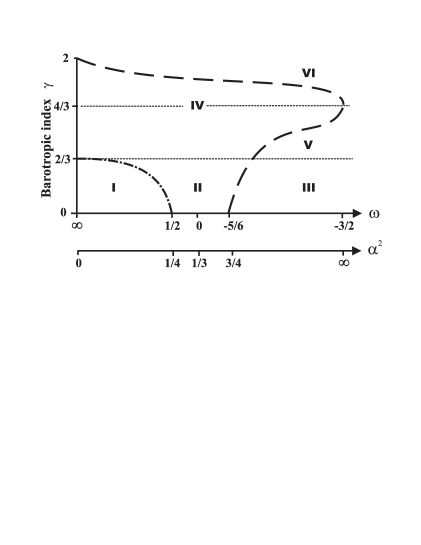
Figure 2: Parameter regimes defined in Section 5. The dashed line represents $\omega_{a}(\gamma)$ and the single dot-dashed line represents $\omega_{*}(\gamma)$.

5.1 Region I:   $\omega_{*}(\gamma)<\omega<\infty\ ,\ \gamma<2/3$.   See Figure 3.

Critical points $(a_{\pm})$ and $(b_{\pm})$ exist at finite values of $x$ and $y$, with point $(a_{+})$ being the stable late-time attractor on the $x+y>0$, $k=0$ separatrix. This parameter regime is inflationary as point $(a_{+})$ corresponds to accelerated expansion and is the attractor solution for all $k\leq 0$ models with $x+y>0$ and a non-zero measure of the $k>0$ models. The remaining $k>0$ trajectories and all $k\leq 0$ models with $x+y<0$ approach one of the vacuum solutions $(c_{-})$ or $(d_{-})$. We find that only those closed ($k>0$) models above a second sepratrix passing through point $(b_{+})$ reach the inflationary solution at late times [24, 25]. For instance, when $\omega=18(1-\gamma)/(2-3\gamma)^{2}$ the second separatrix is the straight line $y=2x/(2-\gamma)$, but we do not have an analytic expression for this separatrix in the more general case.

The generic early-time behaviour is given by the matter dominated solution $a_{-}$ or the vacuum solutions $c_{+}$ or $d_{+}$, while points $b_{\pm}$ and $e_{\pm}$ are saddle points.

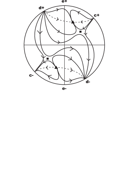
Figure 3: Example of phase-plane in region I ($\gamma=1/3,\omega=6$). The solid triangle represents critical points $(a_{\pm})$. The solid square represents the critical points $(b_{\pm})$. The dashed line is the $k=0$ separatrix.

5.2 Region II:   $\omega_{a}(\gamma)<\omega<\omega_{*}(\gamma)\ ,\ \gamma<2/3$.   See Figure 4.

Critical points $a_{\pm}$ and $b_{\pm}$ exist at finite values of $x$ and $y$. We have marginal inflation as point $b_{+}$ the stable late-time attractor solution for all $k<0$ models with $x+y>0$. All $k>0$ trajectories and $k\leq 0$ models with $x+y<0$ collapse to the vacuum solutions $c_{-}$ or $d_{-}$.

The generic early-time behaviour is given by the scaling solution $b_{-}$ for $k<0$ models with $x+y<0$ or the vacuum solutions $c_{+}$ or $d_{+}$ for $k\leq 0$ trajectories with $x+y>0$ and all $k>0$ models. Points $a_{\pm}$ and $e_{\pm}$ are saddle points.

As $\omega\to\omega_{a}$ from above (and we approach region III) point $(a_{+})$ moves along the $k=0$ separatrix towards point $(c_{+})$ at infinity, and $(a_{-})$ moves off towards $(d_{-})$. On the other hand, as $\gamma\to 2/3$ from below (and we approach region IV) we see that points $(b_{\pm})$ move off towards the curvature dominated solutions at points $(e_{\pm})$.

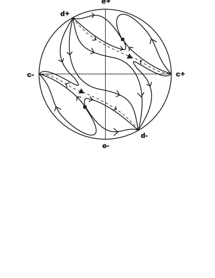
Figure 4: Example of phase-plane in region II ($\gamma=1/3,\omega=0$). Symbols as for Figure 3.

5.3 Region III:   $\omega<\omega_{a}(\gamma)\ ,\ \gamma<2/3$.   See Figure 5.

Only points $b_{\pm}$ now exist at finite values of $x$ and $y$. We have marginal inflation as point $b_{+}$ is the stable late-time attractor for all $k<0$ models with $x+y>0$. All $k>0$ models and $k\leq 0$ trajectories with $x+y<0$ approach the vacuum solution $d_{-}$ at late times. Generic $k=0$ solutions with $x+y>0$ evolve from $d_{+}$ to $c_{+}$ while $k=0$ solutions with $x+y<0$ evolve from $c_{-}$ to $d_{-}$.

The generic early-time behaviour is given by the scaling solution $b_{-}$ for $k<0$ models with $x+y<0$ or the vacuum solution $d_{+}$ for $k\leq 0$ trajectories with $x+y>0$ and all $k>0$ models. Points $c_{\pm}$ and $e_{\pm}$ are saddle points.

As $\gamma\to 2/3$ from below (and we approach region VI) points $(b_{\pm})$ tend towards points $(e_{\pm})$.

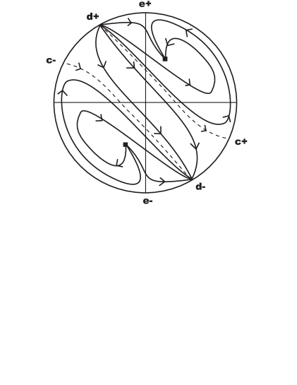
Figure 5: Example of phase-plane in region III ($\gamma=1/3,\omega=-1$). Symbols as for Figure 3.

5.4 Region IV:   $\omega_{a}(\gamma)<\omega<\infty\ ,\ \frac{2}{3}<\gamma<2$.   See Figure 6 and 7.

Only points $a_{\pm}$ exist at finite values of $x$ and $y$. Point $e_{+}$ is the stable late time attractor for $k<0$ solutions with $x+y>0$. All $k>0$ models and $k\leq 0$ trajectories with $x+y<0$ approach one of the vacuum solutions $c_{-}$ or $d_{-}$ at late times. Generic $k=0$ solutions with $x+y>0$ evolve from vacuum solutions $c_{+}$ or $d_{+}$ towards the matter dominated solution $a_{+}$.

The generic early-time behaviour is given by point $e_{-}$ for $k<0$ models with $x+y<0$ or the vacuum solutions $c_{+}$ or $d_{+}$ for $k\leq 0$ trajectories with $x+y>0$ and all $k>0$ models. Points $a_{\pm}$ are saddle points.

For $\gamma<4/3$ we see that as $\omega\to\omega_{a}$ from above (and we approach region V) point $(a_{+})$ moves off towards point $(c_{+})$, and $(a_{-})$ moves off towards $(d_{-})$ at infinity. On the other hand, as $\omega\to\omega_{a}$ from above for $\gamma>4/3$ (and we approach region VI) point $(a_{+})$ moves off towards point $(d_{+})$, and $(a_{-})$ moves off towards $(c_{-})$ at infinity.

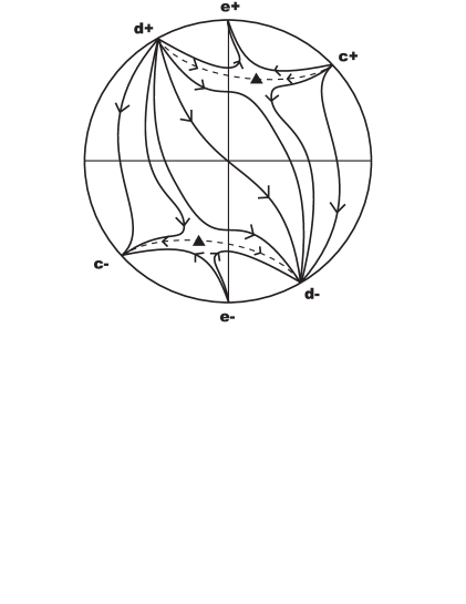
Figure 6: Example of phase-plane in region IV when $\gamma<4.3$ (here $\gamma=1,\omega=6$). Symbols as for Figure 3.

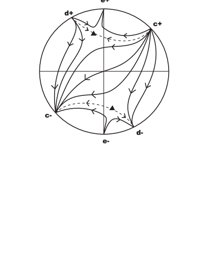
Figure 7: Example of phase-plane in region IV when $\gamma>4.3$ (here $\gamma=1.5,\omega=6$). Symbols as for Figure 3.

5.5 Region V:   $\omega<\omega_{a}(\gamma)\ ,2/3<\gamma<4/3$.   See Figure 8.

There are no critical points at finite values of $x$ and $y$. Point $e_{+}$ is the stable late time attractor for $k<0$ solutions with $x+y>0$. All $k>0$ models and $k\leq 0$ trajectories with $x+y<0$ approach the vacuum solution $d_{-}$ at late times.

The generic early-time behaviour is given by point $e_{-}$ for $k<0$ models with $x+y<0$ or the vacuum solutions $d_{+}$ for $k\leq 0$ trajectories with $x+y>0$ and all $k>0$ models. Points $c_{\pm}$ are saddle points.

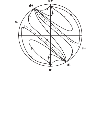
Figure 8: Example of phase-plane in region V ($\gamma=1,\omega=-17/12$). Symbols as for Figure 3.

5.6 Region VI:   $\omega<\omega_{a}(\gamma)\ ,4/3<\gamma<2$.   See Figure 9.

There are no critical points at finite values of $x$ and $y$. Point $e_{+}$ is the stable late time attractor for $k<0$ solutions with $x+y>0$. All $k>0$ models and $k\leq 0$ trajectories with $x+y<0$ approach the vacuum solution $c_{-}$ at late times.

The generic early-time behaviour is given by point $e_{-}$ for $k<0$ models with $x+y<0$ or the vacuum solutions $c_{+}$ for $k\leq 0$ trajectories with $x+y>0$ and all $k>0$ models.

Points $d_{\pm}$ are saddle points.

Figure 9: Example of phase-plane in region VI ($\gamma=3/2,\omega=-17/12$). Symbols as for Figure 3.

6 Non-singular evolution

In general relativity it is well-known that all spatially flat or open ($k\leq 0$) FRW models with a barotropic fluid have a semi-infinite lifetime and posseess a singularity either at a finite cosmic time in the past (for expanding models) or in the future (contracting solutions) so long as $\gamma>0$. Closed models ($k>0$) have a finite lifetime with both a past and a future singularity unless $\gamma<2/3$ in which case non-singular evolution, i.e., infinite proper lifetime, is possible.

It is natural to ask whether in the context of Brans-Dicke gravity it is possible to have a non-singular universe in open or flat models, and/or for $\gamma>2/3$. Our phase-plane analysis provides a qualitative description of the asymptotic evolution that is possible in the different parameter regimes in terms of the time parameter $\tau$, and equations (4.16) and (4.40) relate the asymptotic behaviour of $\tau$ to the proper cosmic time $t$.

As $\omega\to\infty$ the critical points $(a_{+})$ and $(b_{+})$ with $x_{i}+y_{i}>0$ follow the pattern described above for expanding models in general relativity with semi-infinite proper lifetimes. Point $(b_{+})$, whenever it exists ($\gamma<2/3$), always describes a solution with a past singularity, but continuing in to the infinite future. Point $(a_{+})$ similarly describes a semi-infinite lifetime solution with past singularity for $\omega>{\rm max}\{\omega_{a},\omega_{-}\}$. Points $(a_{-})$ and $(b_{-})$ are just the time-reversed solutions of points $(a_{+})$ and $(b_{+})$ respectively, and thus are also semi-infinite but with the future singularities. This suggests that solutions which interpolate between points $(a/b_{-})$ and $(a/b_{+})$ would have an infinite lifetime, but the phase-plane plots show that the solutions which cross the line $x+y=0$ always start from a critical point with $x_{i}+y_{i}>0$ and end up at a critical point $x_{j}+y_{j}<0$ which would yield a finite lifetime. These are analogous to the closed models in general relativity which evolve from a past singularity to a future singularity.

However for $\omega_{a}<\omega<\omega_{-}$ (which is possible for $1<\gamma<4/3$) the solution at point $(a_{+})$ extends to the infinite past and the singularity lies in the future, whereas it is the point $(a_{-})$ which has a singularity in the past. But in this case we find no trajectories which link point $(a_{+})$ to point $(a_{-})$. (Points $(b_{\pm})$ do not exist in this parameter regime.)

Solutions at the fixed points $(a)$ or $(b)$ are necessarily singular to the past or future with semi-infinite lifetime because they correspond to power-law evolution for the scale factor, except when $\omega=\omega_{a}(\gamma)$. In this particular case the scale factor expands exponentially and the solutions at points $(a_{\pm})$ is indeed non-singular. However in this case the solution is unstable as points $(a_{\pm})$ are saddle points in the phase-plane.

Generic solutions in the phase-plane interpolate between two of the critical points including at least one of the vacuum solutions $(c_{\pm})$, $(d_{\pm})$ or $(e_{\pm})$ at infinity. As $\omega\to\infty$ points $(c_{+})$ and $(d_{+})$ are early-time attractors [$f\theta<0$ in equation (4.37)] as $\tau\to\tau_{*}$ and this corresponds to a singularity at finite time $t_{*}$ [$F(\theta)>0$ in equation (4.40)]. For $\gamma<2/3$ point $(e_{+})$ is also an early-time attractor with a singularity at a finite time $t_{*}$, but for $\gamma>2/3$ point $(e_{+})$ becomes a late-time attractor where $t\to+\infty$ as $\tau\to\tau_{*}$. For all values of $\gamma$ we are unable to construct non-singular trajectories as $\omega\to\infty$. The situation is actually worse than in general relativity plus barotropic fluid due to the presence of the scalar field. Even in the limit $\omega\to\infty$ the Brans-Dicke field leads to singular evolution at early or late times even in closed models when $\gamma<2/3$.

However for $\omega_{a}(\gamma)<\omega<-4/3$, which is possible for $\gamma>1$, we have $t\to-\infty$ at point $(c_{+})$ which is still an early-time attractor. Thus trajectories in this parameter regime that originate at point $(c_{+})$, which has no past singularity, are non-singular if they connect to a critical point with no future singularity. We find three parameter regions in which non-singular trajectories occur:

1. $\omega_{a}<\omega<\omega_{-}$

   • Open models ($k<0$) can originate at point $(c_{+})$ in the infinite past and approach point $(e_{+})$ in the infinite future.

2. ${\rm max}\{\omega_{-},\omega_{a}\}<\omega<-4/3$

   • Open models ($k<0$) can originate at point $(c_{+})$ in the infinite past and approach point $(e_{+})$ in the infinite future.

   • Flat models $(k=0$) can originate at point $(c_{+})$ in the infinite past and approach point $(a_{+})$ in the infinite future.

   • Closed models ($k>0$), with $\gamma>4/3$, can originate at point $(c_{+})$ in the infinite past and approach point $(c_{-})$ in the infinite future.

3. $\omega<{\rm min}\{\omega_{-},-4/3\}$

   • Open models ($k<0$) originate at point $(c_{+})$ in the infinite past and approach point $(e_{+})$ in the infinite future.

   • Flat models $(k=0$) originate at point $(c_{+})$ in the infinite past and approach point $(d_{+})$ in the infinite future.

   • Closed models originate at point $(c_{+})$ in the infinite past and approach point $(c_{-})$ in the infinite future.

Note that the time reverse of these solutions linking points $(e_{-})$ and $(c_{-})$, etc., will also be non-singular in the appropriate parameter regime.

We should stress that an infinite proper lifetime is a necessary, but not sufficient, condition for these solutions to be non-singular. In particular, Kaloper and Olive [36] have recently emphasised that as the metric is, by definition, only minimally coupled to the other fields in the Einstein frame, gravitational waves follow geodesics in this frame. Thus if the solutions have a singularity in the finite past in terms of the proper time in the Einstein frame, defined in Eq. (2.8), they may still be geodesically incomplete. One can show that all the critical points with $x_{i}+y_{i}>0$ have singularities at a finite proper time in the past, and extend into the infinite future, in the Einstein frame.

7 Summary

We have constructed an autonomous phase-plane describing the evolution of the scale factor and Brans-Dicke field for FRW cosmologies containing a barotropic fluid in Brans–Dicke gravity. We have improved upon previous phase-plane analyses [25] by presenting all the FRW models in a single phase-plane. We are thus able to present a qualitative analysis of the general evolution of homogeneous and isotropic cosmologies in Brans-Dicke gravity, recovering previously known power-law solutions as fixed points in the phase-plane. These fixed points correspond to self-similar evolution [23]. This is possible due to the scale-invariance of the Brans-Dicke gravity theory which contains no characteristic value for the Brans-Dicke field, $\Phi$.

We find four critical points at finite values of the phase-plane when $\gamma<2/3$ and $\omega>\omega_{a}(\gamma)$ [see Eq. (4.18)]. Two of the fixed points correspond to Nariai’s power-law solutions [29], $a\propto t^{p}$, $\Phi\propto t^{q}$, for spatially flat models ($k=0$). One of these fixed points is expanding $y>0$ and the other is contracting $y<0$. The remaining two fixed points describe a novel self-similar curvature-scaling evolution for spatially curved models [24, 25], with $a\propto t$ and $\Phi\propto t^{2-3/\gamma}$.

Nariai’s expanding solution is only an attractor at late times if $\omega>\omega_{*}(\gamma)$ [see Eq. (4.21)]. This corresponds to power-law inflationary solutions with exponent $p>1$ and a non-zero measure of spatially curved models approach this flat-space solution. For instance, for a false vacuum energy density ($\gamma=0$) we have $\omega_{*}=1/2$. On the other hand, for a given value of $\omega$ the necessary condition for inflation becomes $\gamma<\gamma_{*}(\omega)$, where [7, 24], from Eq. (4.21),

$$\gamma_{*}(\omega)\equiv{2\over 3}\left(2-\sqrt{{2\omega+3\over 2\omega}}\right)\ ,$$ (7.1)

which is always stronger than in general relativity ($\omega\to\infty$) where $\gamma_{*}=2/3$. For $\gamma_{*}(\omega)<\gamma<2/3$ the expanding curvature-scaling solution with $k<0$ is a late-time attractor for $k<0$ models.

For $\gamma>2/3$ and $\omega>\omega_{a}(\gamma)$ only the two critical points corresponding to Nariai’s solutions remain at finite values in the phase-plane, while for $\gamma<2/3$ but $\omega<\omega_{a}(\gamma)$ only the curved space fixed points remain. For $\gamma>2/3$ and $\omega<\omega_{a}(\gamma)$ their are no fixed points in the finite phase-plane.

By projected the infinite phase-plane onto a unit disc we studied the asymptotic behaviour of solutions at infinity where the fluid density becomes negligible. Here we recover vacuum solutions corresponding to the slow and fast branches of O’Hanlon and Tupper’s vacuum solutions [28] for $k=0$, and the Milne universe for $k<0$ models. The expanding Milne universe is a late-time attractor (and the collapsing solution is an early-time atractor) for $\gamma>2/3$.

We have seen that it is only possible to construct solutions with infinite proper lifetimes for values of the Brans-Dicke parameter $\omega<-4/3$. However, in all cases the solutions possess a curvature singularity in the conformally related Eisntein frame.

References

-
[1]
Jordan P 1947 Ann. der Phys. 1 219: 1959 Z. Phys.
157 112
Fierz M 1956 Helv. Phys. Acta 29 128. - [2] Brans C and Dicke R H 1961 Phys. Rev. 124 925.
- [3] Will C 1993 Theory and Experiment in Gravitational Physics (Cambridge: Cambridge University Press).
- [4] Bergmann P G 1968 Int. J. Theor. Phys. 1 25.
- [5] Wagoner R V 1970 Phys. Rev. D 1 3209.
- [6] Nordtvedt K 1970 Astrophys. J. 161 1059.
- [7] Barrow J D and Maeda K 1990 Nucl. Phys. B341 294.
- [8] Santos C and Gregory R 1997 Annals Phys. 258 111.
- [9] Damour T and Nordtvedt K 1993 Phys. Rev. Lett. 70 2217: Phys. Rev. D 48 3436.
- [10] Green M B, Schwarz J H and Witten E 1988 Superstring Theory (Cambridge: Cambridge University Press).
- [11] Applequist T, Chodos A and Freund P G O 1987 Modern Kaluza-Klein Theories (Redwood City: Addison-Wesley).
-
[12]
Mathiazhagan C and Johri V B 1984 Class. Quantum Grav. 1 L29
La D and Steinhardt P J 1989 Phys. Rev. Lett. 62 376. - [13] Gasperini M and Veneziano G 1993 Astropart. Phys. 1 317.
- [14] Levin J J and Freese K Nucl. Phys. 1994 B421 635.
-
[15]
Starobinsky A and Yokoyama J 1994 in Proceedings of “The Fourth
Workshop on General Relativity and Gravitation”, ed. K. Nakao et al (Yukawa Institute for Theoretical Physics, Kyoto University, 1994)
García-Bellido J and Wands D 1995 Phys. Rev. D 52 5636. -
[16]
Casas J A García-Bellido J and Quiros M 1992 Mod. Phys. Lett.
A7 447: Phys Lett B278 94
Serna A and Alimi J M 1996 Phys. Rev. D 50 7304
Santiago D I, Kalligas D and Wagoner R V Phys. Rev. D 56 7627. - [17] Gurevich L E Finkelstein A M and Ruban V A 1973 Astrophys. Space Sci. 22 231.
- [18] Morganstern R E 1971 Phys. Rev. D4 946
- [19] Morganstern R E 1971 Phys. Rev. D 4 282.
- [20] Lorenz-Petzold D 1984 Astrophys. and Space Sci. 98 249.
- [21] Barrow J D 1993 Phys. Rev. D D 47 5329.
- [22] Mimoso J P and Wands D 1995 Phys. Rev. D 51 477: ibid D 52 5612.
- [23] Wainwright J and Ellis G F R 1997 Dynamical Systems in Cosmology (Cambridge: Cambridge University Press).
- [24] Wands D 1993 Cosmology of Scalar–Tensor Gravities, University of Sussex D.Phil. thesis.
- [25] Kolitch S J and Eardley D M 1995 Annals Phys. 241 128: 1996 ibid 246 121.
- [26] Dicke R H 1962 Phys. Rev. 125 2163.
-
[27]
Maeda K 1989 Phys. Rev. D 39 3159
Wands D 1994 Class. Quantum Grav. 11 269. - [28] O’Hanlon J and Tupper B O J 1972 Il Nuovo Cimento 7 305.
- [29] Nariai H 1968 Prog. Theor. Phys. 40 49.
- [30] Veneziano G 1991 Phys. Lett. B265 287.
- [31] Lidsey J E 1995 Phys. Rev. D 52 5407.
- [32] Brustein R and Veneziano G 1994 Phys. Lett. B329 429
- [33] Halliwell J J (1987) Phys. Lett. B185.
- [34] Burd A B and Barrow J D 1988 Nucl. Phys. B308 929.
- [35] Mukhanov V F, Feldman H A and Brandenberger R H 1992 Phys. Rep. 215 205.
- [36] Kaloper N and Olive K A 1998 Phys. Rev. D 57 811.