Vassiliev invariants: a new framework for quantum gravity

Abstract

We show that Vassiliev invariants of knots, appropriately generalized to the spin network context, are loop differentiable in spite of being diffeomorphism invariant. This opens the possibility of defining rigorously the constraints of quantum gravity as geometrical operators acting on the space of Vassiliev invariants of spin nets. We show how to explicitly realize the diffeomorphism constraint on this space and present proposals for the construction of Hamiltonian constraints.

I Introduction

Quantum gravity presents a fundamental problem: it is a theory with an infinite number of degrees of freedom, and yet it is “topological” in the sense of being invariant under diffeomorphisms. This makes the description of the theory particularly troublesome. In particular, if one recourses to structures of intrinsic topological nature, they tend to have a discrete character that makes them incompatible with the demands of a field theory with an infinite number of degrees of freedom. To put this discussion in a more concrete setting, let us concentrate on the canonical formulation of quantum gravity in terms of the new variables introduced by Ashtekar. In terms of these variables one can construct a representation of the quantum theory purely in terms of loops (the loop representation), and a suitable basis for describing quantum states is given by spin networks. That is, quantum states are labelled by spin networks, multivalent graphs embedded in three dimensional space, with a system of weights associated to each side of the graph. If one imposes the diffeomorphism constraint, one considers functions of the diffeomorphism class of a spin network. There exists a precise sense in which one can endow such a space with an inner product [1], in terms of which spin network states are orthonormal.

In this context, there exists a proposal for the action of the Hamiltonian constraint of quantum gravity due to Thiemann [2]. In such a proposal the Hamiltonian constraint weighed by a lapse is just given by a topological operator acting at the vertices of the spin networks. The Hamiltonian constraint commutes with itself, as it is expected it should happen in a diffeomorphism invariant context. The construction also allows for the inclusion of matter in the theory in a well defined regularized framework. It has been observed [3], however, that if one considers Thiemann’s Hamiltonian as acting on a larger space of functions (that are not diffeomorphism invariant), the Hamiltonian constraint continues to commute with itself. Although one can arrange the right hand side of the commutator to also vanish, it appears that the price to pay is tantamount to having a degenerate metric [4]. It also appears that this result is rather generic, holding for many possible detailed forms of the action of the Hamiltonian at vertices. Other non-local proposals also seem to suffer of difficulties with the constraint algebra [5].

On the other hand over the last few years, a variety of formal results have been obtained on a different space of states, that in which the loop derivative is well defined. In particular, a proposal for the Hamiltonian constraint of quantum gravity in terms of loop derivatives exists, and it has been shown that at a formal level the classical Poisson brackets are reproduced by the quantum theory [6]. The main drawback of this space of states is twofold: on the one hand there is the fact that the loop derivative does not appear to exist on generic diffeomorphism invariant states. This is due to the fact that such states change discontinuously when one changes the loops and therefore one cannot introduce a differential operator in loop space. Moreover, definitions of the Hamiltonian in terms of the loop derivative have only been attempted in the context of multiloops (not spin networks). In this context, each type of loop and intersection has to be treated individually, and therefore most results (for instance proofs that certain states were annihilated by the constraints) were only of a partial nature.

The purpose of this paper is to notice that there exist a set of especially important knot invariants that appear to have the property of being loop differentiable. As a consequence, one can operate on them in terms of the Hamiltonian and diffeomorphism constraints of quantum gravity written in terms of loop derivatives in a more systematic way. The invariants in question are the Vassiliev invariants, which in turn are conjectured [7] to be complete enough to be able to separate knots. Moreover, they have recently been generalized to the spin network context [8]. We will show explicitly that these invariants are annihilated by the diffeomorphism constraint of quantum gravity written in terms of loop derivatives. We will also start the analysis of the action of the regularized Hamiltonian constraint of the theory. All of this will be done in terms of spin networks, which allows us to discuss in a unified way all types of intersections and loops.

The organization of this paper is as follows. In section II we discuss the Vassiliev invariants and their loop differentiability. In section III we discuss the action of the diffeomorphism constraint. In section IV we analyze proposals for the Hamiltonian constraint.

II Preliminaries

A Quantum states

The kind of states we will consider as candidates of interest for physical states in quantum gravity has a long motivation in attempts to try to show that there is a loop space representation counterpart of the Chern–Simons state in quantum gravity (see [9] for references). To briefly summarize, one considers general relativity written in terms of Ashtekar’s new variables, which consist of a canonical pair given by a set of densitized triads $\tilde{E}^{a}_{i}$ and a (complex) $SU(2)$ connection $A_{a}^{i}$. If one considers a quantum representation in which wavefunctions are functions of the connection $\Psi[A]$, it is known that if one considers a wavefunction given by,

$$\Psi[A]=\exp\left({ik\over 4\pi}\int{\rm Tr}(A\wedge\partial A+{2\over 3}A\wedge A\wedge A\right)=\exp\left(ikS_{CS}\right)$$ (1)

is annihilated [10, 11] by all the constraints of quantum gravity with a cosmological constant $\Lambda=24\pi/k$.

One can now consider a loop representation, obtained by expanding the states of the connection representation in terms of a basis of states given the traces of the holonomies built with the connection (Wilson loops). In terms of such a basis, the wavefunction we considered above would be given by,

$$\Psi[\gamma]=\int DA\exp(ikS_{CS})W(\gamma,A)$$ (2)

where $\gamma$ is a loop. This integral can be thought of in a different context, as the expectation value of the Wilson loop in a Chern–Simons theory. Such integrals have been the subject of a lot of studies. It is known that the integral is related with a knot polynomial that is a regular isotopy invariant (a framing dependent knot invariant) known as the Kauffman bracket. It is also known that all the framing information is concentrated in an overall factor proportional to the exponential of the self-linking number of the knot. If one removes this overall factor one is left with a polynomial that is closely related to the Jones polynomial, which is ambient isotopic invariant (a genuine invariant under diffeomorphisms) [12]. These polynomials appear evaluated for a particular value of their variable, usually denoted as $q$. The particular value is $q=\exp(2\pi i/k)$, with $k$ being the coupling constant of the Chern–Simons theory. The resulting expressions are presented not as polynomials but as infinite series in $1/k$. The coefficients of these series are known to be Vassiliev invariants [7, 13, 14]. Although these results have never been derived using rigorous measure theory, they have been used extensively to construct solutions to the constraint equations. It was noted that one could write the constraints of quantum gravity in the loop representation in terms of differential operators in loop space involving the loop derivative, and that one can (formally) act with these operators on states as the one listed above. The end result of these manipulations was that one can show that the exponential of the self-linking number is annihilated by the Hamiltonian constraint with a cosmological constant and that the second coefficient of the expansion in $1/k$ of the Jones polynomial is annihilated by the vacuum (zero cosmological constant) Hamiltonian constraint. This coefficient is a Vassiliev invariant.

All these results had several shortcomings. When one works in the loop representation one needs to ensure that wavefunctions satisfy a series of identities stemming from the fact that the loop basis consists of traces of $SU(2)$ matrices. These identities are called Mandelstam identities and in general imply very complex relations between the values of functions of loops. Therefore if one wants to consider a knot invariant as a possible candidate for a state of quantum gravity in the loop representation, one needs to ensure that such invariant satisfy the Mandelstam identities. Although this was the case for the second coefficient we discussed above, it appeared as unlikely that higher coefficients would satisfy the identities. Moreover, the proofs that a certain coefficient was annihilated by the constraint were performed for very special types of intersections (the Hamiltonian constraint only acts nontrivially at intersections). Part of the intention of this paper is to show that similar results are present in the spin network context, where all types of intersections can be treated in a unified fashion. A key to generalizing these results has been the recent observation that ambient isotopic invariants (genuine invariants under diffeomorphisms) can also be defined in terms of spin networks [8].

B Spin networks

Spin networks are constructed considering graphs that are embedded in three dimensions. The graphs are multi-connected with intersections that can be tri-valent or of higher valence. Each connecting line is associated with a holonomy of the connection $A_{a}^{i}$ in a given representation of the group in question (in our case, $SU(2)$, representations are labelled by a (half)integer). One can construct a generalization of the trace of the holonomy (Wilson loop) which we call Wilson net, by considering the traces of the holonomies along the Wilson nets joined by appropriate “intertwiners” at the intersections. The intertwiners consist of invariant tensors in the group. There are several possibilities of how to connect the invariant tensors and the holonomies and this has led to different conventions in the definition of the spin networks. The convention we will choose will follow closely that of Witten and Martin [15, 16], and differs of those of other authors in the field [17, 2, 18].

Consider a multi-connected graph embedded in three dimensions. In order to associate a holonomy to each line in the graph, we need to associate an orientation to each line, so from now on we will consider oriented graphs, with each line associated with a number which labels the representation in which we are considering the holonomy along such a line. The next task is to assign the intertwiners at each intersection. Let us consider trivalent graphs. For graphs of higher valence, one can choose a decomposition of the higher order intersections into superpositions of graphs with trivalent ones [17]. At each intersection one can have several possibilities, depending on if the lines are all incoming, all outgoing or some are ingoing and some outgoing. Let us consider the case of either all ingoing or all outgoing lines. In those cases, there exist two ways of contracting the holonomies with the $3jm$ symbol which intertwines them, given that the latter is cyclic in its three entries. We will label one of the possibilities “$+$” and the other “$-$” and we will refer to them as the “orientations” of the vertex. For a positive orientation we therefore have that the intertwiner is,

$$\raisebox{-28.45274pt}{\psfig{height=56.9055pt}}=\raisebox{-28.45274pt}{\psfig{height=56.9055pt}}=\left(\begin{array}[]{ccc}j_{1}&j_{2}&j_{3}\\ m_{1}&m_{2}&m_{3}\end{array}\right),$$ (3)

whereas for a negative orientation we have,

$$\raisebox{-28.45274pt}{\psfig{height=56.9055pt}}=\raisebox{-28.45274pt}{\psfig{height=56.9055pt}}=\left(\begin{array}[]{ccc}j_{1}&j_{3}&j_{2}\\ m_{1}&m_{3}&m_{2}\end{array}\right)=(-1)^{j_{1}+j_{2}+j_{3}}\left(\begin{array}[]{ccc}j_{1}&j_{2}&j_{3}\\ m_{1}&m_{2}&m_{3}\end{array}\right).$$ (4)

It is useful to introduce a tensor notation. In this notation we denote the intertwiners as $V$ and use lower indices to denote outgoing lines whereas upper indices denote ingoing lines. Therefore,

$$V_{j_{1}m_{1}\,j_{2}m_{2}\,j_{3}m_{3}}=V^{j_{1}m_{1}\,j_{2}m_{2}\,j_{3}m_{3}}=\left(\begin{array}[]{ccc}j_{1}&j_{2}&j_{3}\\ m_{1}&m_{2}&m_{3}\end{array}\right).$$ (5)

Holonomies are also associated with tensorial objects, which we denote by $U$. These objects are labelled by the appropriate representation of the group $j$ and have two indices, the upper index is associated to the point of departure and the lower index to the point of arrival, i.e., $U^{(j)}{}^{n}{}_{n}$. There is a metric tensor that allows to raise and lower index,

$$\epsilon^{(j)}{}^{n\,n^{\prime}}=\epsilon^{(j)}{}_{n\,n^{\prime}}=\left(\begin{array}[]{ccc}j&j&0\\ n&n^{\prime}&0\end{array}\right)=(-1)^{j-n}\delta^{n}_{-n^{\prime}}.$$ (6)

With this metric we can now obtain the intertwiners for trivalent vertices with mixed ingoing/outgoing lines,

$$= V_{j_{1}m_{1}\,j_{2}m_{2}}{}^{j_{3}m_{3}}=\epsilon^{(j_{3})}{}^{m_{3}m^{\prime}_{3}}V_{j_{1}m_{1}\,j_{2}m_{2}\,j_{3}m^{\prime}_{3}}$$ (7)

$$= V^{j_{1}m_{1}\,j_{2}m_{2}}{}_{j_{3}m_{3}}=\epsilon^{(j_{3})}{}_{{m^{\prime}}_{3}m_{3}}V^{j_{1}m_{1}\,j_{2}m_{2}\,j_{3}m^{\prime}_{3}}.$$ (8)

As an example of our conventions, let us consider, the evaluation of the Wilson net for the so called “theta diagram” spin network,

$$\raisebox{-28.45274pt}{\psfig{height=56.9055pt}}=V_{j_{1}n_{1}\,j_{2}n_{2}\,j_{3}n_{3}}U^{(j_{1})}{}^{n_{1}}{}_{m_{1}}U^{(j_{2})}{}^{n_{2}}{}_{m_{2}}U^{(j_{3})}{}^{n_{3}}{}_{m_{3}}V^{j_{1}m_{1}\,j_{2}m_{2}\,j_{3}m_{3}}.$$ (9)

We have therefore provided a definition of the Wilson net for any spin network. One simply constructs an invariant with holonomies and invariant tensors as the ones described above.

With the above definition, the Wilson net has certain properties. In particular there is a dependence on the Wilson net on the orientation of the vertices. What we will now do is modify the definition in order to have an invariant that does not depend on the orientation of the vertices. This will correspond to the normalization of the Wilson net given by Witten and Martin. What we do is multiply the definition introduced up to now times a factor given by,

$$V_{\pm}=\exp\left(\pm{i\pi\over 2}[j_{1}+j_{2}+j_{3}]\right)\sqrt[4]{(2j_{1}+1)(2j_{2}+1)(2j_{3}+1)}$$ (10)

for each vertex in the spin network. With this factor, one can show that the Wilson net defined is invariant under changes from $+$ to $-$ type vertices. It is worthwhile noticing that in the work of Kauffman and Lins [18] on invariants of spin networks the normalization is different.

C Knot invariants for spin networks

We wish to study invariants that represent the transform of the Chern–Simons state into the spin network basis. That is, we are interested in expressions of the form,

$$E(\Gamma,k)=\int DA\exp(ikS_{CS})W(\Gamma,A)$$ (11)

where $\Gamma$ is a spin network and $W(\Gamma,A)$ is the Wilson net we introduced in the previous subsection. This kind of integral has been analyzed using monodromy techniques [15, 16] and variational techniques [19, 20]. The result is a regular isotopic invariant of spin networks. The techniques do not give a unique answer for the invariant, but there are several possibilities, tantamount to having several definitions for the measure $DA$. Each possibility is uniquely characterized by prescribing a value for the invariant on the so called theta-net. The choice of Witten and Martin [15, 16] is,

$$\Theta(j_{1},j_{2},j_{3})=E\left(\raisebox{-35.56593pt}{\psfig{height=71.13188pt}}\,,\,k\right)=\sqrt{\Delta_{1}\Delta_{2}\Delta_{3}},$$ (12)

with,

$$\Delta_{j}=E\left(\raisebox{-14.22636pt}{\psfig{height=28.45274pt}}\,,\,k\right)={q^{j+{1\over 2}}-q^{-j-{1\over 2}}\over q^{1\over 2}-q^{-{1\over 2}}},$$ (13)

and as we mentioned above, $q=\exp(2\pi i/k)$.

The definition of the invariant $E(\Gamma,k)$ is completely given in [20], one needs to supplement the above definitions with relations for recoupling and for crossings of the invariant. The resulting invariant is regular isotopic, meaning that it is not invariant under the elimination of twists. Specifically,

$$E\left(\raisebox{-28.45274pt}{\psfig{height=56.9055pt}}\,,\,k\right) = (-1)^{j_{1}+j_{2}+j_{3}}\exp\left(i\pi(h_{1}+h_{2}-h_{3})\right)E\left(\raisebox{-28.45274pt}{\psfig{height=56.9055pt}}\,,\,k\right),$$ (14)

$$E\left(\raisebox{-28.45274pt}{\psfig{height=56.9055pt}},k\right) = \exp\left(-2\pi ih_{j}\right)E\left(\raisebox{-28.45274pt}{\psfig{height=56.9055pt}},k\right)=\exp\left(2\pi ih_{j}\right)E\left(\raisebox{-28.45274pt}{\psfig{height=56.9055pt}},k\right),$$ (15)

where $h_{i}\equiv{j_{i}(j_{i}+1)\over 2k}$.

These moves correspond to diffeomorphisms, therefore the invariant constructed is not invariant under diffeomorphisms. In other words, the invariant is diffeomorphism invariant of ribbons and not of ordinary loops. One needs a framing (a prescription for assigning a ribbon to each loop) to have a well defined invariant.

However, it was noted early on in the context of loops, and later in the context of spin networks [8], that the dependence on framing can be concentrated on an overall factor. In order to isolate this factor, one simply considers a power series expansion in $\kappa=(2\pi i)/k$ and extracts the linear coefficient in $\kappa$. That coefficient, exponentiated, is the overall factor. This construction is discussed in detail in [8], where it is shown that it indeed leads to an ambient isotopic invariant, in other words, a genuine diffeomorphism invariant function of loops. The resulting invariant is then given by,

$$E(\Gamma,\kappa)=E(\Gamma,0)\exp\left(v_{1}(\Gamma)\kappa\right)P(\Gamma,\kappa)$$ (16)

where $P(\Gamma,\kappa)$ is a spin network generalization of the Jones polynomial (it reduces to it when $\Gamma$ is a simple loop in the fundamental representation) and $v_{1}$ is the first coefficient in the expansion in powers of $\kappa$ (for a single loop it reduces to the self-linking number). The factor $E(\Gamma,0)$, which corresponds to the evaluation of the invariant for $\kappa=0$, contains information about the coloring of the graph, and no information about the embedding. It can be thought of as the evaluation of the Wilson net for a flat connection.

It was shown by Alvarez and Labastida [21] in the case of $\Gamma$ being simple loops, and later generalized for links, that the invariant $E(\Gamma,\kappa)$ can be written as the exponential of a linear combination of primitive Vassiliev invariants,

$$E(\Gamma,\kappa)=E(\Gamma,0)\exp\left(\sum_{i=1}^{\infty}\sum_{j=1}^{d_{i}}\alpha_{ij}(\Gamma)r_{ij}(G)\kappa^{i}\right)$$ (17)

where $\alpha_{ij}(\Gamma)$ are the primitive Vassiliev invariants, which are only dependent on the embedding of the loop (they are independent of the gauge group of the Chern–Simons theory). $d_{i}$ is the number of primitive Vassiliev invariants of order $i$, $G$ is the gauge group (for our case $SU(2)$), and $r_{ij}$ are group-dependent coefficients. We will assume that a similar structure appears for the case of generic $SU(2)$ spin networks, specifically

$$E(\Gamma,\kappa)=E(\Gamma,0)\exp\left(\sum_{i=1}^{\infty}v_{i}(\Gamma)\kappa^{i}\right).$$ (18)

That is, we assume that the invariant is still given by the exponentiation of a set of “Vassiliev” invariants for spin nets, but we are not decomposing the expression in terms of “primitive” invariants, which is a structure that at present is not known in the spin network context. The $v_{i}(\Gamma)^{\prime}s$ are ambient isotopic for $i>1$.

By constructing these invariants of spin networks, we have bypassed one of the main obstacles that working with loops and links had in this context: how to comply with the Mandelstam identities. The invariants of spin nets we have constructed automatically take care of this. An important missing element in the spin network context is the idea of how “generic” is the set of $v_{i}(\Gamma)^{\prime}s$. In the context of loops it is conjectured that the primitive Vassiliev invariants are enough to distinguish all knots. In the case of spin networks we are not working with primitive invariants and therefore it is questionable how generic the basis of invariants one is considering is. This is important if one is making the case that these invariants are the “arena” where one is going to discuss quantum gravity. If a decomposition in terms of primitive invariants of the exponential were known, the techniques we will develop will still be applicable. However, since up to present it is not known how to do this decomposition we will work with the $v_{i}$’s. It is worthwhile pointing out that the techniques we will introduce later in this paper to operate with loop derivatives and diffeomorphism constraints are geometrical in nature and not group dependent. Since it is known that all Vassiliev invariants can be constructed from the Chern–Simons integral with arbitrary groups, and our technique is not group dependent, we therefore have a de-facto method to operate on all Vassiliev invariants. For concreteness we will in the current paper concentrate on the case of $SU(2)$.

III Loop differentiability of the Vassiliev invariants

The loop derivative [9] is a differential operator in loop space that arises by considering two loops that differ by an infinitesimal element of area as “close”. It acts on basepointed objects (either loops or spin networks) by adding a path starting at the basepoint up to a point $x$, where it introduces an infinitesimal planar loop, and retraces back to the basepoint. The definition is,

$$(1+\sigma^{ab}\Delta_{ab}(\pi_{o}^{x}))\Psi(\gamma)=\Psi(\gamma\circ\delta\gamma)$$ (19)

where $\pi$ is a path from the origin to $x$, and the loop $\gamma\circ\delta\gamma$ is shown in figure 1

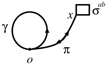
FIG. 1.: The loop that defines the loop derivative

and $\sigma^{ab}=\delta u^{[a}\delta v^{b]}$ is the infinitesimal element of area spanned by the two vectors $\vec{u}$ and $\vec{v}$ defining the parallelogram one adds at the end of the path $\pi$. For a spin network, acting at a line on the network, the definition is exactly the same as for loops, except that the path becomes a line of the same valence as the line on which the basepoint lies, and the infinitesimal loop is also of the same valence as the path.

We now wish to apply the loop derivative to the invariants we introduced in the previous section. A priori one expects that such a quantity does not exist. In particular, for a generic knot invariant, the loop derivative indeed does not exist. This is due to the fact that knot invariants are discontinuous functions in the space of loops. Loop derivatives change the topology of loops (for instance, they can remove intersections [11]), and therefore the limit defining the derivative is ill defined. What we will show here is that due to the properties of the invariants of Chern–Simons under deformations of the loops given by the skein relations, one can introduce a reasonable definition of the loop derivative for these kinds of invariants. It is similar to try to define the derivative of a discontinuous functions by allowing the derivative to take value in the distributions. We will analyze the consistency of this result with the properties of the invariants. The strategy is as follows. The invariants are defined as a functional integral of a Wilson net with a weight function. The only dependence on the spin net is in the Wilson net, so we will assume that the loop derivative of the invariant is equal to the functional integral of the action of the loop derivative on the Wilson net, with the appropriate weight factor,

$$\Delta_{ab}(\pi_{o}^{x})E(\Gamma,\kappa)\equiv\int DA\exp(ikS_{CS}[A])\Delta_{ab}(\pi_{o}^{x})W(\Gamma,A).$$ (20)

Here we have assumed that the limit defining the loop derivative and the one defining the path integral are interchangeable.

The starting point of the calculation is the action of the loop derivative on a holonomy (in the $j$ representation of $SU(2)$) associated to an edge $e_{A}^{B}$ of the spin network, containing the basepoint $o$,

$$\Delta_{ab}(\pi_{o}^{x})U^{(j)}(e_{A}^{B})^{m}{}_{n}=[U^{(j)}(e_{A}^{o})U^{(j)}(\pi_{o}^{x})F^{(j)}_{ab}(x)U^{(j)}({\pi^{-1}}_{o}^{x})U^{(j)}(e_{o}^{B})]^{m}{}_{n},$$ (21)

and the fundamental relation satisfied by the Chern–Simons state,

$$F^{(j)}_{ab}(x)\exp({ik}S_{CS}[A])=-{4\pi i\over k}\epsilon_{abc}{\delta\over\delta A_{c}^{(j)}(x)}\exp({ik}S_{CS}[A]).$$ (22)

So the idea works exactly in the same way it did for ordinary loops [11, 22], the loop derivative acting on a holonomy produces an $F_{ab}$, which can be re-expressed as a functional derivative acting on the exponential of the Chern–Simons form. The last step is to perform a formal integral by parts of the functional derivative and have it act on the holonomies of the spin network that were left by the action of the loop derivative. The end result is,

$$\Delta_{ab}(\pi_{o}^{x})E(\Gamma,\kappa) = -2\kappa\sum_{e_{C}^{D}\in\Gamma}\epsilon_{abc}\int_{e_{C}^{D}}dy^{c}\delta^{3}(x-y)\times$$ (24)

$$<\cdots U^{(j)}(e_{A}^{o})U^{(j)}(\pi_{o}^{x})\tau^{J}_{(j)}U^{(j)}({\pi^{-1}}{}_{o}^{x})U^{(j)}(e_{o}^{B})\cdots U^{(k)}(e_{C}^{y})\tau^{J}_{(k)}U^{(k)}(e_{y}^{D})\cdots>_{CS}$$

where $\tau^{J}_{(j)}$ are the $SU(2)$ generators in the $j$ representation, and the expectation value is assumed to be taken with respect to the measure $DA\exp(iS_{CS})$ and the dots refer to the fact that we just highlight the portion of the spin network where the loop derivative acts. It is understood that the products of holonomies continue until the net is closed and the appropriate traces are taken. A pictorial representation of the quantity within the expectation value is given in figure 2.

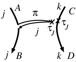
FIG. 2.: The loop derivative acting on a spin network

The above expression can be rearranged using the Fierz identity,

$$\sum_{I=1}^{3}[\tau_{(k)}^{I}]_{s}^{t}[\tau_{(j)}^{I}]_{r}^{q}={1\over 2}\sum_{l=|j-k|}^{j+k}(2l+1)\rho_{l}(j,k)\raisebox{-28.45274pt}{\psfig{height=56.9055pt}},$$ (25)

where $\rho_{l}=l(l+1)-j(j+1)-k(k+1)$, and where the dotted line denotes that the two vertices are at the same point, i.e. the line between the two vertices carries a holonomy equal to the identity.

Using the rearrangement, we get,

$$\Delta_{ab}(\pi_{o}^{x})E(\Gamma,\kappa)=-\sum_{e_{C}^{D}\in\Gamma}\kappa\sum_{l=|j-k|}^{j+k}(2l+1)\rho_{l}(j,k)\epsilon_{abc}\int_{e_{C}^{D}}dy^{c}\delta^{3}(x-y)\left<\raisebox{-28.45274pt}{\psfig{height=56.9055pt}}\right>{}_{\raisebox{-8.53581pt}{$\scriptstyle CS$}},$$ (26)

and then using the basic recoupling property of $SU(2)$ spin networks,

$$\raisebox{-28.45274pt}{\psfig{height=56.9055pt}}=\sum_{m=0}^{2j}(-1)^{2j}(2m+1)\raisebox{-28.45274pt}{\psfig{height=56.9055pt}},$$ (27)

we get,

$$\Delta_{ab}(\pi_{o}^{x})E(\Gamma,\kappa)=-\sum_{e_{C}^{D}\in\Gamma}\kappa\sum_{l=|j-k|}^{j+k}\sum_{m=0}^{2j}(-1)^{2j}(2m+1)(2l+1)\rho_{l}\epsilon_{abc}\int_{e_{C}^{D}}dy^{c}\delta^{3}(x-y)\left<\raisebox{-28.45274pt}{\psfig{height=56.9055pt}}\right>{}_{\raisebox{-8.53581pt}{$\scriptstyle CS$}}$$ (28)

and applying recoupling in the dotted circle in (28) and using the 6j symbols, one gets the final expression,

$$\Delta_{ab}(\pi_{o}^{x})E(\Gamma,\kappa)=\sum_{e_{C}^{D}\in\Gamma}\sum_{m=0}^{2j}-\kappa\epsilon_{abc}\int_{e_{C}^{D}}dy^{c}\delta^{3}(x-y)\lambda^{\pm}_{m}(j,k)\left<\raisebox{-28.45274pt}{\psfig{height=56.9055pt}}\right>{}_{\raisebox{-8.53581pt}{$\scriptstyle CS$}},$$ (29)

where,

$$\lambda^{\pm}_{m}(j,k)=(-1)^{j\mp k}\sum_{l=|j-k|}^{j+k}(-1)^{l-(m\mp m)/2}(2m+1)(2l+1)\rho_{l}\left\{\begin{array}[]{ccc}j&j&m\\ k&k&l\end{array}\right\}.$$ (30)

So the end result is that the loop derivative acting on the invariant $E(\Gamma,\kappa)$ is nonvanishing only if the endpoint of the path $\pi_{o}^{x}$ of the loop derivative falls upon one of the lines of the spin network. The end result is, up to a factor, proportional to the invariant $E(\Gamma^{\prime},\kappa)$, where $\Gamma^{\prime}$ is a new graph obtained by adding the path $\pi_{o}^{x}$ to the original graph $\Gamma$. Notice that the action of the loop derivative is covariant under diffeomorphisms, in the sense that a diffeomorphism would shift both the graph $\Gamma$ and the path $\pi_{o}^{x}$ and therefore would act as a diffeomorphism on the graph $\Gamma^{\prime}$. It is also worthwhile noticing that the general form of equation (29) is true for any gauge group, the only differences would appear in the recoupling coefficients $\lambda$ and the corresponding irreducible representations associated with the graph. This emphasises the geometrical nature of the action of the loop derivative and may open possibilities for generalizing this construction for invariants that do not necessarily arise from $SU(2)$ groups. The importance of this is that it appears that Vassiliev invariants for spin nets might arise as linear combinations of products of “primitive” invariants associated only with the topological embedding of the graph of the spin net, times some group-dependent factors that contain information about the valences of each line in the spin net. The loop derivative acts on such objects by ignoring the group prefactors and acting on the factors depending on the embedding of the spin net diagrams. In particular, if one acts on $E(\Gamma,0)$, since it does not have information about the embedding, the loop derivative automatically gives zero.

The loop derivative as defined in this paper has several appealing properties that other differential operators in loop space do not have (see [9] for more details). One property we wish to emphasize is that the loop derivative satisfies Leibnitz’ rule. It acts on a product of functions exactly like an ordinary derivative. This allows, when evaluating operators on products of knots (as for instance when we extract the frame dependent prefactor and the $E(\Gamma,0)$), to perform explicit calculations.

For instance, we can compute the action of the loop derivative on any Vassiliev invariant of type $v_{n}$, by computing the logarithmic derivative of $E(\Gamma,\kappa)$. The final result is,

$$\Delta_{ab}(\pi_{o}^{x})v_{n}(\Gamma)=-\sum_{e_{j}\in\Gamma}\sum_{m=0}^{2j}\lambda_{m}\epsilon_{abc}\int_{e_{j}}dy^{c}\delta^{3}(x-y){E(\Gamma_{m},0)\over E(\Gamma,0)}{1\over(n-1)!}\left[{d^{n-1}\over d\kappa^{n-1}}\exp\left(\sum_{r}\left(v_{r}(\Gamma_{m})-v_{r}(\Gamma)\right)\kappa^{r}\right)\right]_{\kappa=0}$$ (31)

and the action is nonvanishing only if $o,x$ fall on two different lines of $\Gamma$ and the spin net $\Gamma_{m}$ is obtained by taking $\Gamma$ and adding to it the line $\pi_{o}^{x}$ with valence $m$.

IV The diffeomorphism constraint

A The operator

In this section we will introduce the diffeomorphism constraint as a differential operator in loop space written in terms of the loop derivative. We will also show that the invariants we introduced in the previous section will be either annihilated by the constraint in the case of ambient isotopy invariants, or will transform appropriately in the case of regular isotopic invariants.

Let us consider the diffeomorphism constraint of quantum gravity written in terms of Ashtekar’s new variables,

$$\hat{C}(\vec{N})\Psi[A]=\int d^{3}xN(x)^{a}\hat{\tilde{E^{b}_{i}}}(x)\hat{F}_{ab}^{i}(x)\Psi[A].$$ (32)

Because this expression involves the product of two operators at the same point, in general we need to regularize it, which we do via a point splitting function $\lim_{\epsilon\rightarrow 0}f_{\epsilon}(x,y)=\delta^{3}(x,y)$,

$$\hat{C}(\vec{N})\Psi[A]=\lim_{\epsilon\rightarrow 0}\int d^{3}x\int d^{3}y\,f_{\epsilon}(x,y)N^{a}(x)\hat{\tilde{E}}^{b}_{i}(x)[U(\pi_{x}^{y})\hat{F}_{ab}(y)U^{-1}(\pi_{y}^{x})]^{i}\Psi[A]$$ (33)

where in order to preserve gauge invariance we have connected the $F_{ab}$ and $\tilde{E}$ operators with holonomies along a path $\pi$ going from $x$ to $y$.

The above operator, when acting on a Wilson net, can be rewritten in terms of the loop derivative, as has been discussed in the context of loops in the past [9]. The explicit expression is,

$$\hat{C}(\vec{N})W(\Gamma,A)=\lim_{\epsilon\rightarrow 0}\int d^{3}x\,f_{\epsilon}(x,y)\sum_{e_{A}^{B}\in\Gamma}\int_{e_{A}^{B}}dy^{b}N^{a}(y)\Delta_{ba}(\pi_{y}^{x})W(\Gamma,A).$$ (34)

One can explicitly check that the action of this operator is a diffeomorphism, provided that the connection $A$ is smooth. In the limit in which the regulator is removed, the path $\pi$ shrinks to a point and one ends with a loop with an infinitesimal closed loop attached at the point $x$. The addition of this closed loop is tantamount to displacing infinitesimally the line of the original loop at the point $x$.

We will now assume that the generator of diffeomorphisms has in general the form given by equation (34) in terms of the loop derivative and we will show that when acting with it on the invariants from Chern–Simons we get the correct result. This result is nontrivial, since in the path integral that defines the invariant there are contributions from distributional connections.

B Action on regular isotopic invariants

To discuss in a cleaner fashion the action of the diffeomorphism operator on the invariants, we will consider diffeomorphisms in which the vector $\vec{N}$ has compact support. This will allow us to focus on the action of diffeomorphisms on individual edges, on vertices, etc, each at a single time. It is immediate that a generic situation can be analyzed combining all results we will derive. Let us start with the action at an individual line, (we define $\hat{C}(\vec{N})=\lim_{\epsilon\rightarrow 0}\hat{C}_{\epsilon}(\vec{N})$)

$$\hat{C}_{\epsilon}(\vec{N})\left<\raisebox{-28.45274pt}{\psfig{height=56.9055pt}}\right>{}_{\raisebox{-8.53581pt}{$\scriptstyle CS$}} = \kappa\sum_{m=0}^{2j}\lambda^{-}_{m}(j,j)\int dy^{b}\int dz^{c}f_{\epsilon}(z,y)\epsilon_{abc}N^{a}(z)\times$$ (36)

$${1\over 2}[\Theta(z-y)\left<\raisebox{-28.45274pt}{\psfig{height=56.9055pt}}\right>{}_{\raisebox{-8.53581pt}{$\scriptstyle CS$}}+\Theta(y-z)\left<\raisebox{-28.45274pt}{\psfig{height=56.9055pt}}\right>{}_{\raisebox{-8.53581pt}{$\scriptstyle CS$}}],$$

where $\Theta$ are Heaviside functions that order points along the line of the spin net we are considering. One can easily define them introducing a parameterization. We now use a recoupling identity,

$$\left<\raisebox{-28.45274pt}{\psfig{height=56.9055pt}}\right>{}_{\raisebox{-8.53581pt}{$\scriptstyle CS$}}={(-1)^{2j}\over(2j+1)}\{j,j,m\}\left<\raisebox{-28.45274pt}{\psfig{height=56.9055pt}}\right>{}_{\raisebox{-8.53581pt}{$\scriptstyle CS$}}$$ (37)

where $\{j,j,m\}$ is the $3j$ symbol that is zero unless the $j$ and $m$ values satisfy the triangular relation at the vertices. We now remove the regulator, assuming the following regularization function,

$$f_{\epsilon}(y,z)={3\over 4\pi\epsilon^{3}}\Theta(\epsilon-|z-y|).$$ (38)

Evaluating the integral, one gets,

$$\hat{C}(\vec{N})\left<\raisebox{-28.45274pt}{\psfig{height=56.9055pt}}\right>{}_{\raisebox{-8.53581pt}{$\scriptstyle CS$}}={\kappa\over 8\pi}\sum_{m=0}^{2j}\lambda^{-}_{m}(j,j){(-1)^{2j}\over(2j+1)}\int_{0}^{1}ds\,\epsilon_{abc}{\dot{N}(s)^{a}\dot{y}(s)^{c}\ddot{y}(s)^{b}\over|\dot{y}(s)|^{3}}\left<\raisebox{-28.45274pt}{\psfig{height=56.9055pt}}\right>{}_{\raisebox{-8.53581pt}{$\scriptstyle CS$}}$$ (39)

where we have introduced a parameterization such that $dy^{a}=\dot{y}(s)^{a}ds$ and dots refer to total derivatives with respect to $s$. We can summarize the above result by saying that, for diffeomorphisms of compact support acting on lines of the spin net, we have that,

$$\hat{C}(\vec{N})E(\Gamma,\kappa)=\kappa\mu(j)w(\vec{N})E(\Gamma,\kappa)$$ (40)

where $\mu(j)=\sum_{m=0}^{2j}\lambda^{-}_{m}(j,j){(-1)^{2j}\over(2j+1)}$ is a recoupling factor, that depends on the weight of the line in question, and $w(\vec{N})$ is the writhe introduced in the line by the action of the diffeomorphism along the vector $\vec{N}$. We therefore see that the diffeomorphism has a well defined limit. The result is dependent on a background metric through the writhe, as expected for a regular istopic invariant. Notice that the result decomposes as a product of a factor depending entirely on the “coloring” of the spin net and another factor depending only on the embedding of the net in three dimensions. What we have therefore recovered is a formula that contains the information about the non-invariance of $E(\Gamma,k)$ under the addition of twists, given by the skein relation (15). This skein relation could be reobtained exactly by exponentiating the action of the loop derivative, as discussed in [22], but we will not repeat the calculation here for brevity.

Let us now consider the action of the diffeomorphism at an intersection. Here we get, in addition to the contributions we discussed for a single line, a contribution when the end of the path of the loop derivative intersects one of the lines entering the intersection. We have,

$$\hat{C}(\vec{N})\left<\raisebox{-28.45274pt}{\psfig{height=56.9055pt}}\right>{}_{\raisebox{-8.53581pt}{$\scriptstyle CS$}}=\kappa\sum_{\alpha\neq\beta=1}^{3}\sum_{m=0}^{2j_{\alpha}}\lambda^{-}_{m}(j_{\alpha},j_{\beta})\int dy^{b}\int dz^{c}f_{\epsilon}(y,z)N^{a}(z)\epsilon_{abc}\left<\raisebox{-28.45274pt}{\psfig{height=56.9055pt}}\right>{}_{\raisebox{-8.53581pt}{$\scriptstyle CS$}},$$ (41)

and using the recoupling identity,

$$\left<\raisebox{-28.45274pt}{\psfig{height=56.9055pt}}\right>{}_{\raisebox{-8.53581pt}{$\scriptstyle CS$}}={(-1)^{m+j_{\gamma}-j_{\alpha}-j_{\beta}}\left\{\begin{array}[]{ccc}j_{\alpha}&j_{\beta}&m\\ j_{\beta}&j_{\alpha}&j_{\gamma}\end{array}\right\}\over\Theta(j_{\alpha},j_{\beta},j_{\gamma})}\left<\raisebox{-28.45274pt}{\psfig{height=56.9055pt}}\right>{}_{\raisebox{-8.53581pt}{$\scriptstyle CS$}},$$ (42)

and removing the regulator as before, we get,

$$\hat{C}_{\epsilon}(\vec{N})\left<\raisebox{-28.45274pt}{\psfig{height=56.9055pt}}\right>{}_{\raisebox{-8.53581pt}{$\scriptstyle CS$}}=\kappa\sum_{\alpha=1}^{2}\sum_{\beta=\alpha+1}^{3}\Omega_{m}(j_{\alpha},j_{\beta},j_{\gamma})\epsilon_{abc}\dot{N}^{a}(0)\dot{y}^{b}_{\alpha}(0)\dot{y}^{c}_{\beta}(0)\left<\raisebox{-28.45274pt}{\psfig{height=56.9055pt}}\right>{}_{\raisebox{-8.53581pt}{$\scriptstyle CS$}}$$ (43)

where,

$$\Omega_{m}(j,k,l)=Q(-1)^{m+l-j-k}\left\{\begin{array}[]{ccc}j&k&m\\ k&j&l\end{array}\right\}\lambda^{-}_{m}(j,k)$$ (44)

with $Q$ a constant given by,

$$Q={1\over 4\pi}\int_{0}^{\pi/2}d\phi{(\sin\phi-\cos\phi)\over\sqrt{|\dot{\vec{y}}_{\alpha}(0)|^{2}\cos^{2}\phi+|\dot{\vec{y}}_{\beta}(0)|^{2}\sin^{2}\phi-2|\dot{\vec{y}}_{\alpha}(0)\cdot\dot{\vec{y}}_{\beta}(0)|\cos\phi\sin\phi}}.$$ (45)

In the above equations we have assumed a parameterization with parameter equal to zero at the intersection. The geometrical meaning of this expression is that it vanishes if the volume spanned by the two tangents at the intersection and the derivative of the vector $\vec{N}$ along one of the lines entering the intersection vanishes. If this volume is nonzero, we start to reconstruct infinitesimally the twist at the intersection covered by the skein relation (14). Again, one could recover it exactly exponentiating the action of the loop derivative as described in [22].

C Action on ambient isotopic invariants

Here we will show that the diffeomorphism operator we introduced vanishes when acting on the ambient isotopic invariants, concretely $P(\Gamma,\kappa)$. Therefore, it annihilates every Vassiliev invariant. In order to compute the action, let us recall equation (18),

$$E(\Gamma,\kappa)=E(\Gamma,0)(1+v_{1}(\Gamma)\kappa+(2v_{2}(\Gamma)+v_{1}(\Gamma)^{2}){\kappa^{2}\over 2}+\cdots)$$ (46)

and analyze the action of the diffeomorphism on $E(\Gamma,\kappa)$ order by order in $\kappa$. To order zero we get,

$$\hat{C}(\vec{N})E(\Gamma,0)=0$$ (47)

which is correct, since $E(\Gamma,0)$ does not depend on the embedding of the spin net, just on its coloring, and it is immediately annihilated by the loop derivative. At the next order, we have,

$$\hat{C}(\vec{N})v_{1}(\Gamma)=\mu(j)w(\vec{N})$$ (48)

where we have assumed the diffeomorphism as acting on an isolated line of valence $j$, a similar formula holds for the intersections with a different coloring weight. As before $w(\vec{N})$ is the writhe induced in the line by the vector field $\vec{N}$. If we now take advantage of the fact that the diffeomorphism operator satisfies Leibnitz’ rule, we see that combining (40) and (48) we get,

$$\hat{C}(\vec{N})\exp(-\kappa v_{1}(\gamma))E(\Gamma,\kappa)=0,$$ (49)

and therefore we see that indeed the diffeomorphism constraint annihilates all Vassiliev invariants, namely,

$$\hat{C}(\vec{N})P(\Gamma,\kappa)=\hat{C}(\vec{N})\exp\left(\sum_{n=2}^{\infty}v_{n}(\Gamma)\kappa^{n}\right)=0.$$ (50)

Since the diffeomorphism constraint annihilates all Vassiliev invariants, it also annihilates any function of the Vassiliev invariants. As we mentioned before, there are indications that Vassiliev invariants may constitute a basis of diffeomorphism invariant functions of loops. What we have shown here is that the definition of the loop derivative we introduced in the spin network context is compatible with that fact, namely it naturally leads to a diffeomorphism constraint that annihilates explicitly all Vassiliev invariants.

V Towards a Hamiltonian constraint

Let us now consider the Hamiltonian constraint of quantum gravity, possibly with a cosmological constant $\Lambda$,

$$\hat{H}(M\hbox to0.0pt{\hss\lower 8.61108pt\hbox{$\widetilde{\hphantom{M}}$}})=\int d^{3}xM\hbox to0.0pt{\hss\lower 8.61108pt\hbox{$\widetilde{\hphantom{M}}$}}\left[\epsilon^{ijk}\hat{\tilde{E}}^{a}_{i}\hat{\tilde{E}}^{b}_{j}\hat{F}_{ab}^{k}+{\Lambda\over 6}\epsilon^{ijk}\hat{\tilde{E}}^{a}_{i}\hat{\tilde{E}}^{b}_{j}\hat{\tilde{E}}^{c}_{k}\epsilon_{abc}\right].$$ (51)

This expression corresponds to the “doubly densitized” operator. We chose to do this since we have experience with this operator from the context of loops [9] and it is easily expressed in terms of the loop derivative. We will later suggest how one could transform this expression into a single densitized version. We need to regularize the operator, which again we do through a point splitting. There are many options as to how to exactly point split. The way we do it, for the $\Lambda=0$ piece, is,

$$g_{\epsilon,\epsilon^{\prime},\epsilon^{\prime\prime}}(u,v,w,x)H(u,v,w)\equiv g_{\epsilon,\epsilon^{\prime},\epsilon^{\prime\prime}}(u,v,w,x)\epsilon^{ijk}\hat{\tilde{E}}^{a}_{i}(u)\hat{\tilde{E}}^{b}_{j}(v)[U(\pi_{u}^{w})F_{ab}(w)U(\pi_{w}^{u})]^{k}.$$ (52)

So we have chosen to join the $F_{ab}$ with one of the $E$’s via a holonomy. There are many other possibilities (for instance, joining all operators via holonomies, which would yield a gauge invariant regularization) and they all yield the same classical expression in the the limit $\epsilon\rightarrow 0$. A possible regulating function is defined as,

$$g_{\epsilon,\epsilon^{\prime},\epsilon^{\prime\prime}}(u,v,w,x)=f_{\epsilon}(x,u)f_{\epsilon}(x,{u+v\over 2})f_{\epsilon}(x,{u+v+w\over 3})$$ (53)

with $f$ defined as in the diffeomorphism constraint. This regulating function is the same as the one usually considered for the “Ashtekar–Lewandowski” volume operator, [1, 23]. It is worthwhile pointing out that for the following discussion, this issue is not important, since we will discuss results that do not require to remove the regulator.

To determine the action of the Hamiltonian in terms of spin networks, we consider the action of the operator we have just defined on a Wilson net. As is well known, this operator only acts at intersections of the net. At regular points it gives rise to “acceleration” terms, which we will omit since they vanish on diffeomorphism invariant states [24, 9]. The nonvanishing action comes from the triads acting at two points on different strands $i,k$ entering an intersection $V$,

$$H(u,v,w)W\left(\raisebox{-28.45274pt}{\psfig{height=56.9055pt}},A\right) = -{i\over 2}\sum_{i\neq k\in V}\sum_{m=|i-k|}^{i+k}(2m+1)\rho_{m}(i,k)\int_{e_{i}}dy^{a}\delta^{3}(u-y)\int_{e_{k}}dz^{b}\delta^{3}(v-z)\times$$ (55)

$$\left[\Delta_{ab}(\pi_{y+}^{w})-\Delta_{ab}(\pi_{y-}^{w})\right]W\left(\raisebox{-42.67912pt}{\psfig{height=85.35826pt}},A\right)$$

where in the last diagram all the structure occurs “at a point” and points $y\pm$ are identified.

Having the Hamiltonian in terms of the loop derivative allows to evaluate its action on any of the invariants we have been discussing. Let us start by showing that the Hamiltonian constraint with a cosmological constant term annihilates the invariant $E(\Gamma,\kappa)$. In order to do this, we need to derive an expression for the operator $\hat{\rm det}q$, $q$ being the spatial metric in terms of spin nets. The construction completely parallels that of the Hamiltonian constraint, the operator $\hat{\rm det}q$ is obtained by replacing $F_{ab}^{i}$ in the Hamiltonian with $\epsilon_{abc}\tilde{E}^{c}_{i}$. In order to be possible to have a cancellation with the Hamiltonian, one has to regularize both operators in a similar manner. So we choose,

$$g_{\epsilon,\epsilon^{\prime},\epsilon^{\prime\prime}}(u,v,w,x)\hat{{\rm det}}(u,v,w)\equiv{i\over 3!}g_{\epsilon,\epsilon^{\prime},\epsilon^{\prime\prime}}(u,v,w,x)\epsilon^{ijk}\hat{\tilde{E}}^{a}_{i}(u)\hat{\tilde{E}}^{b}_{j}(v)[U(\pi_{u}^{w})\tilde{E}^{c}(w)U(\pi_{w}^{u})]^{k}\epsilon_{abc}.$$ (56)

The point-splitting (i.e. where one decides to insert each holonomy) could have been made in a different way (e.g. [1, 2]), but one can show —using recoupling theory— that inserting additional holonomies leads in the limit when one removes the regulator to the same result for a given regulating function.

The end result for the operator is,

$$\hat{{\rm det}g}(u,v,w)\Psi\left(\raisebox{-28.45274pt}{\psfig{height=56.9055pt}}\right) = {1\over 24}\sum_{i,k,l}\sum_{m,n}(2m+1)\rho_{m}(i,k)\lambda^{-}_{n}(i,l)\epsilon_{abc}\times$$ (59)

$$\int_{e_{i}}dy^{a}\delta^{3}(y,u)\int_{e_{k}}dz^{b}\delta^{3}(z,v)\int_{e_{l}}dt^{c}\delta^{3}(t,w)\times$$

$$\left[\Psi\left(\raisebox{-34.1433pt}{\psfig{height=71.13188pt}}\right)-\Psi\left(\raisebox{-34.1433pt}{\psfig{height=71.13188pt}}\right)\right].$$

The vertex on which the determinant acts can be of any order, if it is higher than trivalent, the determinant is a sum of the above contribution evaluated for all possible triplets of lines. All linkages in the figure are assumed to be happening “at a point”, so recoupling theory can be applied. An interesting observation is that if the vertex is trivalent, simple recoupling identities show that both contributions are equal and therefore the determinant of the metric vanishes on such vertices (as one would have suspected, given that the volume operator vanishes too).

Using the definition of the above operators, one can start obtaining results. The first thing we notice is that,

$$g_{\epsilon,\epsilon^{\prime},\epsilon^{\prime\prime}}(u,v,w,x)\hat{H}(u,v,w)E(\Gamma,\kappa)=12\kappa ig_{\epsilon,\epsilon^{\prime},\epsilon^{\prime\prime}}(u,v,w,x)\hat{{\rm det}g}(u,v,w)E(\Gamma,\kappa)$$ (60)

and we therefore see that the generalization of the Kauffman bracket to spin networks $E(\Gamma,\kappa)$ is a solution of the Hamiltonian constraint of quantum gravity with a cosmological constant. This is straightforward to see by considering the action of (55) and making explicit the action of the loop derivative, which adds a line to the diagram in such a way that one ends with the same diagrams as in (59).

Another interesting result is to notice that the Hamiltonian vanishes when acting on Vassiliev invariants at trivalent vertices. This can be straightforwardly seen by recalling the action of the loop derivative on a Vassiliev (31), and noting that at a triple intersection, using recoupling, $v_{p}(\Gamma_{j})=v_{p}(\Gamma)$. We are allowed to use recoupling because the loop derivative acts by adding a line “at a point” when evaluated in the action of the Hamiltonian constraint. Therefore the Hamiltonian constraint vanishes at trivalent vertices.

Another important result concerning the action of the Hamiltonian on Vassiliev invariants can again be concluded from studying the explicit action of the loop derivative (31). Combining this expression with (55) one immediately concludes that the action of the “doubly-densitized” Hamiltonian we are considering here is proportional to the “regularized volume” (strictly speaking it is a volume squared) spanned by three of the tangents entering at an intersection [25],

$$\hat{\rm Vol}^{ijk}_{\rm reg}(x,\epsilon,\epsilon^{\prime},\epsilon^{\prime\prime})=\epsilon_{abc}\int_{e_{i}}dy^{a}\int_{e_{j}}dz^{a}\int_{e_{k}}dw^{a}g_{\epsilon,\epsilon^{\prime},\epsilon^{\prime\prime}}(x,y,z,w).$$ (61)

Concretely, acting on a four-valent vertex labelled by $J$, the action of the Hamiltonian is,

$$g_{\epsilon,\epsilon^{\prime},\epsilon^{\prime\prime}}(x,u,v,w)\hat{H}_{\rm double}(u,v,w)v_{n}(\left(\raisebox{-14.22636pt}{\psfig{height=28.45274pt}}\right)=\sum_{I}\sum_{i,j,k\in{\rm Vertex}}\hat{\rm Vol}^{ijk}_{\rm reg}(x,\epsilon,\epsilon^{\prime},\epsilon^{\prime\prime})C^{IJ}V_{n-1}\left(\raisebox{-14.22636pt}{\psfig{height=28.45274pt}}\right)$$ (62)

with $C^{IJ}$ is a proportionality factor depending on the valences of the strands entering the intersection. Similarly, the ranges of the sum in $I$ is determined by the type of intersection. The invariant $V_{n-1}$ is a non-primitive Vassiliev invariant of order $n-1$, it will involve sums of products of primitive Vassiliev invariants of lower orders.

This proportionality opens the attractive possibility of defining a “singly densitized” Hamiltonian by “dividing by the regularized volume”. Having a singly densitized Hamiltonian can potentially lead to a much better defined operator, since its action could possibly be cast in a background-independent manner, as proportional to a Dirac delta. If this construction works, it might therefore be possible to cast the action of the Hamiltonian constraint in terms of an expression along the lines of,

$$H_{\rm single}(x)v_{n}\left(\raisebox{-14.22636pt}{\psfig{height=28.45274pt}}\right)=\delta(x-{\rm Vertex})\sum_{I}d^{IJ}V_{n-1}\left(\raisebox{-14.22636pt}{\psfig{height=28.45274pt}}\right)$$ (63)

with $d^{IJ}$ another constant factor. Having an operator with such a simple action is not only remarkable, but will open the possibility of further consistency checks, like computing the constraint algebra. All these issues are currently under study and evidently further work is needed to complete this program. The computation can be done “on shell” by showing that the Hamiltonian commutes on Vassiliev invariants using the expressions introduced above. It could also be done “off shell” since one has an expression for the Hamiltonian acting on any function that is loop differentiable, and therefore verify commutation relations with the diffeomorphism constraint.

VI Conclusions

The doubly-densitized Rovelli–Smolin Hamiltonian has been studied, written in terms of the loop derivative, since the early days of the new variable formulation in terms of loops. The early work suffered from three main drawbacks: a) the loop derivative was not a well defined operator on diffeomorphism invariant states; b) the quantum states were difficult to construct and the action of the constraint to check explicitly due to the presence of the Mandelstam identities and c) the Hamiltonian was regularization dependent, potentially having problems at the time of computing the quantum commutator algebra of constraints. In this work, largely by going to the language of spin networks, we have made progress in all three points. First of all, we were able to introduce a loop derivative that is well defined when acting on Vassiliev invariants. The loop derivative leads, while input into the usual definition, to a well defined diffeomorphism constraint, with exactly the kind of action on Vassiliev invariants and its regular-isotopic counterparts, as one would expect. The presence of this reasonable-looking loop derivative operator allows us for the first time to actually have a version of the Rovelli–Smolin Hamiltonian written in terms of the loop derivative that actually is a well defined operator on knots. We have checked that several of the formal results obtained in the loop language still go through with the new operator. Better yet, since all the results are in terms of spin network states, we need not concern ourselves anymore with the Mandelstam identities. Finally, since the Hamiltonian has a relatively simple action on Vassiliev invariants, closely related to the volume operator, the possibility is opened of defining a single-densitized Hamiltonian, just by dividing by the operator representing the determinant of the metric. This latter possibility still needs to be studied in detail. However, preliminary results appear as promising. The single densitized operator appears to have a very natural action on the space of knots. This opens the hope that a consistent set of constraints, satisfying the appropriate commutator algebra, might be found. One could think of computing the commutator algebra off-shell, very much along the same lines as in the formal computations of [6], except that now the operators involved are also well defined on-shell (i.e. when the wavefunctions are knot invariants) . The fact that all this occurs while working on the space of Vassiliev knot invariants based on spin networks suggests that this might be an appropriate setting for the discussion of canonical quantum gravity.

- [1] A. Ashtekar, J. Lewandowski, J. Math. Phys. 5, 2170 (1995).
- [2] T. Thiemann, “Quantum spin dynamics I-VI”, gr-qc/9606089-90 and gr-qc/9705017-20.
- [3] J. Lewandowski, D. Marolf, Int. J. Mod. Phys. D (in press).
- [4] R. Gambini, J. Lewandowski, D. Marolf, J. Pullin, Int. J. Mod. Phys. D (in press).
- [5] L. Smolin, “The classical limit and the form of the Hamiltonian constraint in nonperturbative quantum gravity” preprint gr-qc/9609034.
- [6] R. Gambini, A. Garat, J. Pullin, Int. J. Mod. Phys. D4, 589 (1995); see also B. Brügmann, Nucl. Phys. B474, 249 (1996).
- [7] D. Bar-Natan, Topology, 34, 423 (1995); q-alg/9702009.
- [8] R. Gambini, J. Griego, J. Pullin, Phys. Lett. B (to appear).
- [9] Gambini, R., Pullin, J.: “Loops, knots, gauge theories and quantum gravity.” Cambridge: Cambridge University Press, Cambridge (1996).
- [10] H. Kodama, Phys. Rev. D42, 2548 (1990).
- [11] B. Brügmann, R. Gambini, J. Pullin, Nucl. Phys. B385, 587 (1992).
- [12] E. Witten, Commun. Math. Phys 121, 351 (1989).
- [13] J. Baez, Lett. Math. Phys. 26, 43 (1992).
- [14] L. Kauffman, in “Knots and quantum gravity”, J. Baez editor, Oxford University Press, Oxford (1993).
- [15] E. Witten, Nuc. Phys. B322, 629 (1989).
- [16] S. Martin, Nuc. Phys. B338, 244 (1990).
- [17] C. Rovelli, L. Smolin, Nucl. Phys. B442, 593 (1995).
- [18] L. Kauffman, S. Lins, “Temperley–Lieb recoupling theory and invariants of 3-Manifolds”, Annals of Mathematics Studies, Princeton University Press, Princeton (1994).
- [19] R. Gambini, J. Pullin, Commun. Math. Phys. 185, 621 (1997).
- [20] R. Gambini, J. Griego, J. Pullin, Phys. Lett. B413, 260 (1997).
- [21] M. Alvarez, J. M. F. Labastida, Nucl. Phys. B433555 (1995); Erratum B441, 403 (1995); B488, 677 (1997);q-alg/9604010.
- [22] R. Gambini, J. Pullin, Commun. Math. Phys. 185, 621 (1997).
- [23] T. Thiemann, “Closed formula for the matrix elements of the volume operator in canonical quantum gravity”, gr-qc/9606091.
- [24] B. Brügmann, J. Pullin, Nucl. Phys. B390, 399 (1993).
- [25] B. Brügman, Int. J. Theor. Phys. 34, 145 (1995).