Abstract

We summarize the state of the art of the “close approximation” to black hole collisions. We discuss results to first and second order in perturbation theory for head-on collisions of momentarily-stationary and non-stationary black holes and discuss the near-future prospect of non-axisymmetric collisions.

1 Introduction

When two black holes collide, one can distinguish three regimes in the collision with distinct behaviors. Initially, when the black holes are far apart, one can think of them as individual black holes, each with their own horizon. This regime can be well approximated by post-Newtonian analysis [1]. As the black holes approach, they start exerting more significant influence on each other and their structure becomes distorted. Some approximations have also been suggested for this regime [2]. At some point however, the influence is too intense for approximations to work and one enters a fully nonlinear regime, generally perceived as only treatable by full numerical simulations (from here on we will use the name “full numerical” to mean numerical simulations of the Einstein equations without approximations). As is well known, a great numerical effort is currently underway to try to model this regime, a summary being present in this same volume in the talk by Ed Seidel. Towards the end of the collision, the two black holes will not really be two black holes any longer, but will merge into a larger, highly distorted single black hole. This latter part of the collision could be treated using perturbation theory of a single black hole. This has been known for quite some time. Four years ago, Richard Price and I set out to explore this regime of the collision [3]. One can alternatively view what we were trying to do as applicable to black hole collisions for holes that start very close to each other. So close that they are surrounded by a common horizon. Technically, they are therefore a single hole. However, we expected that if we took the same families of initial data that full numerical simulations were using, and extrapolated them to the case of close holes, our technique would yield results against which to benchmark the full numerical simulations. This would make the results useful. What has been found is that the approximation seems to work in a somewhat broader range of parameters than was initially expected, allowing one to make predictions for separations that are, at least in the head-on collision, of the order of $L/m\sim 7$. At the same time, the advances obtained in full numerical simulations have brought the field to a new level of maturity and it is now recognized that there are several important problems ahead before a full numerical in-spiral collision will reliably be available for a large range of parameters. This makes the close limit studies all the more valuable. For some time, they will be the only source of (albeit only approximate) waveforms for certain types of black hole collisions, just when the interferometric detectors are supposed to come online. Moreover, they will be important benchmarks for full numerical simulations. This warrants going into some depth in the analysis of the close limit approximation for collisions of black holes. This talk will provide an overview of current efforts along these lines.

The close-limit portion of collisions of black holes is dominated by a behavior characterized by a single hole “ringing away” the distortions produced by the collision. The type of waveform one gets, therefore, is dominated by the quasinormal ringing of a black hole. These types of waveforms are not the best to be detected with interferometric detectors. Although they are remarkably intense, they consists of short, rapidly dying trains of oscillations, which are not easily pattern-matched out of the noise. Moreover, for ordinary black holes, they tend to be at a frequency much higher than that of typical interferometric detectors. Are they observable at all? Hughes and Flanagan [4], and more recently Creighton [5] have made a detailed study of all possible phases of the collision and the conclusion seems to be that for a signal to noise of about 8, and for collisions with a final Kerr parameter of $0.98$, one would need collisions with a mass of $100$ solar masses for the final ringing to dominate over the in-spiral. This makes direct observation of the waveforms we will discuss rather unlikely, but of course, not completely ruled out. The final angular momenta of collisions is still an unknown quantity, and if it is lower, it would help observability of final ringing. That will also be the case if black holes with a mass of $50$ Solar masses are more common than expected. For a discussion along these lines see [6]. The conservative attitude today is therefore that the kind of waveforms we will discuss are probably of not great interest from the observability point of view. A conservative philosophy can therefore be that the value of the work to be presented arises as potential benchmarks for numerical simulations. We will see that other surprises appear in the way. It can also teach us in its own right things about generic behaviors of black hole collisions and the initial data to be used. In summary, although this approach is unlikely to have the final word about black hole collisions, it can help us gain several unexpected insights. This will be the theme of this talk.

The organization of this paper is as follows. In the next section we will discuss the initial calculations that opened this whole approach, based on a test case for momentarily-stationary black holes. We will then describe how to endow the formalism with “error bars” using second order perturbation theory. In section IV we describe the collision of boosted black holes and black holes with spin and in section V we discuss the prospect for in-spiralling collisions and other issues.

2 A test case: the Misner problem

In the early 60’s Misner [7] presented an exact solution to the initial value problem of general relativity. He noted that if one imposes that the initial data be momentarily stationary, i.e., the extrinsic curvature is zero, the constraint equations reduce to requiring that the scalar curvature of the slice be zero. He then constructed a conformally flat solution to that equation by obtaining a conformal factor that solved the Laplace equation with boundary conditions adapted to two holes connected by a throat. The availability of this explicit analytic solution to the initial value problem made it an ideal test case for studying the close approximation: not only did we have exact initial data, but actually the evolution of this problem in time has been pursued (given the simplicity implied by axial symmetry) since the 60’s by Smarr and his group, and a detailed treatment has been presented in the last years by the NCSA/Potsdam/WashU group [8]. So four years ago Richard Price and I [3] looked at this in detail. Since the slice is conformally flat, one readily finds coordinates in which, if the holes are very close to each other, the exterior of the throats is isometric to the Schwarzschild geometry in isotropic coordinates plus perturbations. One then evolves the perturbations using the traditional formalism for perturbations of a black hole. For this case one finds that perturbations are pure $\ell=2$ in multipolar nature to first order in the expansion parameter, and one can therefore evolve them with the Zerilli equation. This is a linear differential equation for a coordinate invariant combination of the metric perturbations that has the structure of a Klein–Gordon equation in $1+1$ dimensions with a potential. The potential represents the back-scattering of perturbations by the curved geometry of the black hole. The equation is written in terms of the radial $r*$ tortoise coordinate, which covers only the exterior of the black hole, the horizon being at $r*\rightarrow-\infty$. This does not allow the formalism to answer straightforwardly questions about horizon dynamics, etc. The results of evolving the perturbations determined by the initial data given by the Misner geometry are summarized in figure 1.

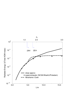
Figure 1.  : The energy released in a head-on collision of momentarily stationary black holes. It is measured in fractions of the total ADM mass of the initial slice and shown as a function of the initial separation of the two holes. The latter is parameterized in two ways, in the top it is given in terms of the $\mu_{0}$ parameter that appears in the explicit form of the Misner geometry, in the bottom it is given in terms of the separation of the throats in the flat conformal space $L$ divided by one half of the ADM mass, as a measure of the “mass of each hole”. We indicate the regions in separation for which there are two separate event and apparent horizons. We plot the results of the close approximation, together with those of full numerical simulations from the NCSA/Potsdam/WashU and the Abrahams-Cook approximation.

In the figure, the continuous curve represents the energy computed using the close approximation. It is worthwhile emphasizing that this curve has no free parameters, that is, once given the initial separation, the Misner data choose a unique evolution and radiated energy. As can be seen the agreement with the numerical results for this problem of the NCSA/Potsdam/WashU group [8] is quite good up to a little after the two holes stop being separated by a common event horizon. That is indicated by the two vertical lines at the top of the plot. To the right of them, there are no common horizons of the type indicated. Given the simplicity of the close limit computation, the results are rather remarkable. Clearly this is a useful benchmark for numerical relativity.

Also shown is the Abrahams and Cook approximation [9]. Theirs is an extension of the close approximation. Their rationale is as follows: suppose you want to collide two black holes at $L/m\sim 10$. Obviously, the close approximation won’t work. How about doing the following: replace the two black holes at $L/m\sim 10$ by two black holes at a distance at which a common horizon has just developed, but with some linear momentum to account to the fact that they “fell in” from $L/m\sim 10$. Evolve the resulting configuration using the “close limit”. How do you compute the momentum? They suggest using Newton theory for two point particles at the equivalent distance and with the equivalent mass. Evidently, there is a very crude approximation done: all the energy radiated during the in-fall is neglected. Yet, as can be seen from the figure, their approximations works very well for large separations. It becomes identical with the close approximation when the two black holes start sharing a common apparent horizon, that explains the strange shape of the Abrahams–Cook curve. One could expect that this approximation would be sensitive to the point where one decides to stop the Newtonian evolution and start to use the “close limit”. This was explored by Baker and Li [10] and the result obtained was that the approximation was quite robust.

Figure 2.  : The perturbative initial data for two colliding black holes and the Zerilli potential. As can be seen, most of the initial data lies at the left of the potential maximum and will tend to be swallowed by the black hole. This is the reason why linearized theory works well in what one would naively presume to be a highly nonlinear situation.

The immediate questions seems to be, why does it work well? Wasn’t the collision of two black holes one of the most nonlinear nontrivial problems in general relativity? How could linearized theory even come close to predicting it? A possible answer can be seen in figure 2. Here we show the initial data and the Zerilli potential plotted as functions of the $r_{*}$ coordinate. As we see, most of the initial data lies within the maximum of the Zerilli potential. As such, it will tend to in-fall into the black hole. Only a small amount escapes to the exterior. Therefore it is not surprising that linearized theory could do a good job. The horizon is actually working for us by “swallowing” the highly nonlinear portions of the problem into the inaccessible regions of the black hole and leaving for the radiative part a weak field, well described by perturbation theory.

The agreement between numerical and approximate predictions is not only confined to energies. There is remarkable agreement in waveforms as well. This is even more surprising, since waveforms have a wealth of information about the collision and again, there is no parameter to fit. We will postpone comparisons of waveforms till we discuss the next section for reasons of space. A long discussion of these comparisons can also be found in [11].

So with the close approximation and the Abrahams-Cook extension one can cover very well (at least qualitatively) the collisions of momentarily stationary black holes. The question then is, can one make progress for other types of collisions? In particular, can one say something about collisions of the physically realistic “in-spiralling” type? We will discuss this in the following sections.

3 Endowing the formalism with error bars

The first problem at hand is the following: yes, one has an approximation. But the domain where one can be “really sure” the approximation is going to work is relatively uninteresting (black holes too close). On the other hand, the results of the test case suggests the approximation works well somewhat beyond this domain. Could one somehow get a better grasp of where the domain of validity lies? The answer we propose to this issue, in collaboration with Reinaldo Gleiser, Oscar Nicasio and Richard Price is to use second order perturbation theory. First order perturbation theory has no way to tell when it is valid. It is only by transcending it and going to second order that one can get a validity check. More important, one can make the validity check useful in terms of the physics one is interested in. For instance, if we are interested in computing radiated energies and waveforms, then we will demand that the second order corrections in those quantities be smaller than the first order ones in order for first order perturbation theory to make sense. The second order corrections can therefore be seen as “rough error bars” of the first order theory predictions. It could happen that other quantities that we are not interested in (for instance, appropriately defined invariant quantities close to the horizon) have quite large second order corrections. But as long as for the quantities of physical interest one can show that higher order corrections are smaller than first order theory predictions, then one has reason to believe those predictions.

Unfortunately, the formalism of higher order perturbations of black holes is much less studied than the first order one. Tomita and Tajima [12] had explored in the seventies second order perturbations, but they did it in a Newman–Penrose approach for studying fields near the horizon. We need a $3+1$ point of view in order to supply the initial data. More importantly, we need a formalism that defines consistent waveforms far away from the black holes. We were able to develop such a formalism. A detailed treatment can be found elsewhere [13, 14]. Basically we repeated step by step the gauge-fixed derivation of the Zerilli equation originally pursued by Zerilli, keeping up to second order terms. The derivation takes place in the Regge–Wheeler gauge, which can be fixed to all orders. One ends up with an equation for a quantity that bears the same relationship on the second order perturbations as the Zerilli function did on the first order perturbations. The equation is exactly the same as the first order Zerilli equation, with the same potential. The only difference is that the equation involves a “source term” that is quadratic in the first order perturbations and that one can rewrite entirely in terms of the first order Zerilli function and its spatial and time (up to third) derivatives. The details can be found in [13]. However, this is not enough. First of all, the “second order Zerilli function” we have just constructed is not a “second order correction” to the first order Zerilli function. They are not terms in the expansion of an exact quantity. They are just combinations of the metric perturbations (in one case first order, in the other case second order) that carry the gauge invariant information of the perturbations (this is not manifest in the gauge fixed approaches we pursue here, but gauge invariant approaches can be constructed as well, in which these functions are gauge invariant). So suppose we compute these functions and their time evolution. What good are they? Without further work, they are of little use. Since they are not the terms of a series expansion, one cannot use them to estimate if perturbations are large or small, i.e., one cannot compare them with each other. What one can do is try to compute waveforms in terms of them. What we did for this was to write the components of the perturbative metric tensor not in the Regge–Wheeler gauge but in a gauge that is manifestly asymptotically flat. In such a gauge one can read directly from the metric functions the “waveforms” an observer far away would measure. One can explicitly compute the relationship between these metric functions to first and second order and the first and second order Zerilli functions we computed. One can then see how much second order terms correct the first order predictions. This is what we were looking for. As a by-product, using the Landau–Lifshitz pseudo-tensor, it is immediate to write expressions for the radiated energy in terms of these asymptotically-flat gauge metric components. This construction was all explicitly done in [13] and it grossly exceeds the space we have here to describe it in detail. So we just summarize it by looking at the results from it. In figure 3 we show the radiated energies for the same problem we discussed in the previous section, the head-on collision of momentarily stationary black holes (“the Misner problem”) but now keeping second order terms [15].

Figure 3.  : The radiated energy for the head-on collision of momentarily stationary black holes, computed to first and second order in perturbation theory compared with the full numerical results. It is clearly seen that second order theory works very well as an “error bar” of the first order formalism.

So we now have a methodology. That is, we can compute the evolution of a given set of initial data for colliding black holes and use second order perturbation theory to estimate how good an approximation to the real result we get. We are therefore ready to attack collisions of further physical interest.

Before we move on to non-momentarily stationary cases, let us mention for completeness that other forms of stationary collisions have also been treated with the close approximation. Abrahams and Price [16] considered the use of “Brill-Lindquist” [17] type initial data. These families of initial data are very similar to Misner’s, but the boundary condition given at the throats is different. In the Misner solution, one requires the geometry to be isometric through the two holes (as if they were connected by a single “handle”) whereas in the Brill-Lindquist case one is considering two holes with different asymptotically flat interior regions. The two boundary conditions, when boiled down to the initial value for the Zerilli equation, only differ in a constant number characterizing the quadrupole term in the expansion in $1/r$ of the conformal factor. This difference becomes more important the closer the black holes are. In spite of being “in the close limit”, for separations of $\mu_{0}>0.8$ or so, the two problems differ in less than a few percent. Andrade and Price [18] considered also the collision of two Brill–Lindquist black holes of unequal mass in the close limit. This allowed them to probe questions such as “is there an optimal mass relation that maximizes radiation?”. Very recent full numerical work of Anninos and Brandt [19] apparently confirm very well the findings of Andrade and Price. Lousto and Price [20] considered the extreme case of one of the black holes being infinitesimally small. This makes contact with previous studies [21] of particles in-falling into black holes. These studies help elucidate certain questions about the initial data. For instance, what sort of boundary conditions for the initial data of two black holes leads in the particle limit to inadequate answers, etc. The conclusion seems to be that, at least for the point-particle limit, the Bowen–York initial data do not work very well. In view of this, Lousto and Price [20] have proposed enhanced initial data that is worthwhile exploring further. All of the above studies have been performed using first order perturbation theory only. Using second order perturbation theory, Gleiser [22] was able to show that the radiated energy and the change in the ADM mass of the system coincide in perturbation theory. These kinds of investigations open the road towards trying to address the back reaction problem in the context of perturbation theory, and more results are expected in the future.

4 Non-momentarily-stationary head-on collisions

The first problem one encounters when trying to address the issue of non-momentarily-stationary collisions is that there are no known exact solutions to the initial value problem of general relativity involving non-vanishing extrinsic curvature. One therefore resorts to the traditional conformal approach. There, one assumes that the three-metric is conformally flat $g_{ab}=\phi^{4}\delta_{ab}$, and to simplify things we take maximal slicing ${\rm Tr}K=0$. If one defines a conformally related extrinsic curvature $\hat{K}_{ab}=\phi^{-2}K_{ab}$ then the diffeomorphism and Hamiltonian constraints simplify to,

$$\nabla_{a}\hat{K}^{ab} = 0$$ (1)

$$\nabla^{2}\phi = -{1\over 8}{\hat{K}^{ab}\hat{K}_{ab}\over\phi^{7}}$$ (2)

where all the derivatives are with respect to flat space.

The usual strategy to solve these equations has been as follows (see for example, the work of Bowen and York [23]): construct a solution to (1) for a single hole in the situation of interest. For instance, Bowen and York present extrinsic curvatures that represent situations that have non-vanishing ADM linear momentum and/or angular momentum. Once you have the extrinsic curvature for a single hole, just superpose two of them to get the extrinsic curvature for two black holes. The momentum constraint is linear, so the resulting extrinsic curvature is still a solution to (1). Plug the resulting extrinsic curvature in (2) and solve the nonlinear elliptic PDE for $\phi$ (usually numerically). Abrahams and Price [24] have studied the issues associated with taking numerical initial data and evolving it using perturbation theory. In fact, the Abrahams–Cook results we discussed before were actually obtained this way.

Here we will pursue a separate avenue [25]. We will solve the constraint equations approximately. After all, our whole formalism is approximate, so we do not really need exact initial data. We will consider the “slow” approximation, where the extrinsic curvature is small. In such a case, one can ignore the right-hand-side of the Hamiltonian constraint (2) and immediately construct a solution to the initial value problem: the extrinsic curvature is the one given by Bowen and York and the conformal factor one takes as if there were no extrinsic curvature. That is, we can borrow the solution of Misner or Brill–Lindquist. From there on, we just apply the techniques we described in the previous sections to do the evolution. If one wants to go to second order, the solution we just presented is a bit too crude, but one can refine it by “feeding back” the extrinsic curvature in the right-hand-side of the Hamiltonian constraint and solving for the conformal factor to second order in the momentum only. This can usually be pursued (at least at each multipolar order $\ell$) analytically.

Can this possibly work? The best answer is given by seeing some results [26]. Let us take a look at the radiated energies for the head-on collision of two black holes boosted towards each other with linear momentum $P$. Figure 4 shows the energy for a given initial separation, in terms of the Misner parameter $\mu_{0}=1.5$. For momentarily-stationary solutions, this was a respectable separation, but not too large (the black holes are surrounded by a common event horizon, not by a common apparent horizon).

Figure 4.  : The radiated energy by the head-on collision of two black holes boosted towards each other, as a function of the momentum, for a separation of $\mu_{0}=1.5,L/m=4.2$. We see good agreement with numerical results for a large range of values of the momentum. We also see the “dip” that occurs for small values of the momentum.

In the figure we see that the energies agree very well with the numerical simulations. But contrary to expected, the approximation does not deteriorate rapidly for large values of $P$. How could this be? Weren’t we performing a “slow” approximation? Evidently there is a surprise here. The surprise is that indeed, our expression for the conformal factor should only work well for small values of $P$. But in the initial data, if one increases $P$, the extrinsic curvature grows linearly in $P$, whereas the conformal factor —tied up by the nonlinearities of the Hamiltonian constraint— only grows very slowly with the momentum. As a result, for large values of $P$, the initial data become “momentum dominated” i.e. swamped by the extrinsic curvature. Since we are inputting the extrinsic curvature exactly, then our approximation actually becomes somewhat better for large values of the momentum. The reason this is not entirely true (and we actually see in the plot that the discrepancy increases with $P$) is that we are inputting exactly $\hat{K}$, the physical extrinsic curvature inherits some error through the conformal factor. But if one is not interested in a great degree of accuracy, it is remarkably simple to provide initial data for this problem. One can set the conformal factor to unity and get reasonable results!

This “momentum dominance” may be an observation that will lead to a lot of implications for realistic collisions. After all, one does not expect that the final moments of a realistic black hole collisions will be well approximated by slices that resemble the Bowen and York initial data (which were constructed in an ad-hoc way). Therefore, there were a lot of worries about what sort of initial data to actually use in numerical simulations, at least if the latter were not to start from very far apart —as surely the initial ones will not.— However, momentum dominance may imply that the situation is not so serious, since for black holes with large values of the momentum —as one expects in realistic collisions—, the ambiguities in the conformal factor of the initial data, could be completely irrelevant, at least if one is interested in performing computations that are not too accurate.

The plot for the energies also shows the “dip” structure for small values of the momentum. This is very counterintuitive. One boosts two black holes towards each other and when they collide they radiate less (in fact almost an order of magnitude less) than if one had let them in-fall from rest. This is a peculiarity of the Bowen–York family of initial data. When one starts boosting the black holes towards each other, one adds extrinsic curvature to the initial data. Waveform-wise, the extrinsic curvature happens to be $180^{\circ}$ out of phase with the conformal factor. Therefore at the beginning they tend to cancel each other. Past a certain point, the extrinsic curvature dominates and the energy increases again. Physically, it appears that a competition is taking place between the added distortions to the geometry the additional momentum supplies and the added size of the horizon which is observed in these families of initial data for increasing momentum [27]. It is like the horizon “jumps out” faster and engulfs more spacetime that could be radiated when one increases the momentum and decreases the amount of radiation produced. It is worthwhile noticing that this effect is linear in $P$, that is, if one reverses the momentum boosting the black holes apart from each other, it is not observed.

Due to reasons of space we can again not detail the second order treatment of boosted black holes we have carried out with Reinaldo Gleiser, Oscar Nicasio and Richard Price. Details can be seen in [28]. Let me just mention that there are several technical complications in the boosted case. It took us almost two years to get the formalism in place. To begin with, the initial data has non-vanishing $\ell=0$ components. One can ignore these to first order —they are pure gauge—, but to second order one needs to take into account the quadratic terms they give rise to. In order to use the formalism we had (which did not include them), one needs to gauge away the $\ell=0$ first order term keeping second order terms in place . This is expensive computationally, but eventually was done. Another issue that arose is that when one considers $\ell=0$ terms, the Regge–Wheeler gauge is not unique. We had to perform a further gauge fixing that is tantamount to a “variable time shift” in the resulting waveforms. Details can be seen in [28]. Moreover, the whole issue of doing perturbation theory when one has more than one parameter (in our case, initial separation and momentum) in the problem, presents additional challenges and can lead to inconsistencies if one is not careful.

The end result, however, is very encouraging. Due to reasons of space I will show only one set of waveforms, for large values of the momentum. Here is where our approximation works the worst, and yet, as can be seen in figure 5, the agreement with the full numerical simulations is remarkably good. In fact, it is probably inconsistent to request any more accuracy from perturbation theory for so large a value of the perturbative parameter.

Figure 5.  : Radiated waveforms for boosted black holes. We see excellent agreement between the predictions of first and second order perturbation theory and the full numerical results, in spite of the fact that this is a very disfavorable case for perturbation theory. The momentum is very large, $P/M_{ADM}\sim 2.44$.

What about black holes with spin? One can consider head-on collisions of spinning black holes rather straightforwardly. For reasons of time, we have not yet completed the analysis of this problem. In fact, this problem appears as much simpler than the boosted black holes problem: there are no $\ell=0$ components, there is no “mixing” between the extrinsic curvature and the conformal factor (at least in first order), since they are of different parity, so there is no “dip” in the energy. Up to now we have only explored it in first order perturbation theory. Results can be seen in [30]. However, because of normalization and other issues, these results are only trustworthy for very small values of the momentum at the moment. In the forthcoming months we expect to present a full analysis including second order results. An interesting development is that Brandt [31] has a full numerical code (developed with Seidel) for evolving distortions of a Kerr black hole and we are working closely with him to compare our evolutions with his for similar families of initial data representing collisions of counter or co-rotating spinning black holes. A result already visible in [30] that might be of interest is that if one aligns the spin along the collision line, the emitted radiation is the maximum. This contradicts a usual expectation, i.e., that axisymmetric situations radiate less than fully non-symmetric ones. This might be an interesting issue to probe as full 3D codes become more stable, since it is an “almost 2D” three dimensional issue.

5 The problem of initial data

As has transpired in the previous sections, the initial data that one constructs to consider black hole collisions following the Bowen–York method might not be what one needs to represent realistic situations. Yet, these data are widely used. Therefore, it is good to get a firm grasp on their physical properties. In particular, it is known that if one considers a single boosted or spinning Bowen–York black hole, one does not end up with a slice of either boosted Schwarzschild nor Kerr. That is, these families of initial data represent boosted/spinning black holes “plus gravitational radiation”. How much radiation is an issue that becomes more pressing the closer one needs to start the collision. For the first numerical simulations it will probably be important, and it is definitely of interest in the close limit. We therefore set out with Reinaldo Gleiser, Oscar Nicasio and Richard Price to estimate the amount of initial radiation present in these solutions to the initial value problem. To do it, we considered a single spinning Bowen–York black hole, and evolved it treating it as a perturbation of Schwarzschild [32]. As long as the angular momentum is small, this is a valid approximation. First order perturbation theory does not yield anything since the first order perturbations are stationary (they account for the fact that one is dealing with a Kerr rather than a Schwarzschild black hole). Nontrivial radiation appears only at second order. With our formalism, we can readily compute this. The result is summarized in figure 6.

Figure 6.  : The energy radiated by a single spinning Bowen–York black hole as it “relaxes” to the Kerr spacetime, as a function of the spin of the hole. We see that for spins greater than $0.6$, it can be comparable to the total energy radiated in a head-on collision.

We see that for spins bigger than $0.6$ in units of ADM mass squared, the radiation present per hole in the initial data can be as large as that emitted in a collision. Unfortunately our technique is not applicable for large values of the spin, but still the result is a cautionary note concerning the use of Bowen–York initial data for large values of momenta.

6 In-spiralling collisions

What can be said about in-spiralling collisions? If one keeps the total angular momentum small, one can even treat these types of collisions as perturbations of a Schwarzschild black hole. One could, for instance, consider the initial data for non-head-on boosted black holes of Bowen–York type and evolve it as a perturbation of Schwarzschild. This was done for first order perturbations in [30]. These results are only credible for quite small angular momenta until we have performed a second order analysis. One sees a similar behavior as in the case of spinning black holes, but the limited range of momenta involved do not allow to draw many conclusions or behaviors. In particular, one really expects more radiation in the case of in-spiralling collisions.

What about trying to treat the problem as a perturbation of the Kerr spacetime? Would this allow to consider cases with larger angular momentum? Perturbations of Kerr have been importantly studied, and the Teukolsky equation is the formalism one would try to use. However, there are several practical and conceptual difficulties that get in the way of trying to do this.

The first practical difficulty is that there was not much experience in working with the Teukolsky equation in the time domain. In such a domain the equation is not entirely separable, and therefore one is left, even after decomposing in spherical harmonics, with a difficult hyperbolic $2+1$-dimensional partial differential equation. Fortunately, work by Krivan, Laguna, Papadopoulos and Andersson [33], who wrote a code for integrating the resulting PDE, now allows us to have at our disposal a tool for the evolution of perturbations of a Kerr black hole that makes the task almost as easy as with the Zerilli equation.

The next two difficulties have to do with properties of the Bowen–York initial data. The first property is that if one considers the extrinsic curvatures of two black holes boosted towards each other in a non-head-on fashion, one can see that it can be rewritten as the extrinsic curvature of a single spinning black hole of angular momentum $L=P\times D$ with $P$ the momenta of each hole and $D$ the impact parameter, plus “perturbations” [34]. Prima facie, this is good. It appears to behave as one expected. However, one quickly notices that both the extrinsic curvature of the spinning black hole and “the perturbations” are of order $P\times D$. That is, if one was hoping that using perturbations of a Kerr hole would allow to treat higher angular momentum cases by “absorbing” the extra angular momentum into the background, this shows that it is not the case. If one increases the angular momentum, perturbations become large. This strikes a blow to the hope that one could do much better using perturbations of Kerr instead of simply perturbations of Schwarzschild. It might be the case that one can do better, but it will not be spectacular. Given the extra complications implied by the Kerr case, it even raises the question of why investing the extra effort for what will appear to be a small payoff. Of course, we can never be sure of how much better we can do until we try it. It could be that numerical coefficients conspire to be small in the right direction, in spite of the terms being of the same “order” in terms of the angular momentum. We shall see.

The other difficulty associated with the Bowen–York type of initial data is related to the fact that the three-metric is conformally flat. There is no explicitly known slicing of the Kerr metric with conformally flat slices. Worse, the Teukolsky equation is explicitly derived in Boyer–Lindquist coordinates, where the slicing is not conformally flat. How does one use the Bowen–York initial data in this formalism? One possibility is to just ignore the issue and define as a perturbation the departure from Boyer–Lindquist that makes the metric conformally flat. This could lead to artificially large perturbations, since one is treating as a perturbation a mismatch in slicing. Again, for small values of the angular momentum, the spatial part of the Kerr metric is approximately conformally flat and therefore this should not be a bad approximation. Treating the Bowen–York data in this way is currently being pursued by Baker, Khanna, Laguna and Pullin [35].

Another way around this latter issue would be to use different families of initial data from that of Bowen and York. It turns out that this is not that easy to do. If one relinquishes conformal flatness, all constraints become coupled and it is difficult to make any sense of a “superposition principle” that would allow to set initial data for two black holes. Some steps in this direction have been recently taken by Baker and Puzio [36] and independently by Krivan and Price [37]. Their constructions at the moment only work for axisymmetric data. But they are non-conformally flat, and have the attractive property of yielding Kerr black holes for far away black holes and a single Kerr black hole in the close limit. At least for head-on collisions of spinning black holes, these new families of initial data hold a lot of promise. Evolution of them is now being studied by the above four authors using the Teukolsky numerical code mentioned above.

Finally, a more technical, but yet practically important issue associated with perturbations of Kerr is that because they had never been studied in the time domain, no one had derived formulas giving the Teukolsky function and its time derivatives in terms of a three metric and an extrinsic curvature. The calculation is complicated given the nontrivial nature of the background, but by now it has been completed independently by Campanelli, Lousto, Krivan, Baker and Khanna [38], who now have formulae suitable for practical use.

Summarizing, we can expect over the next year or so progress in close limit of in-spiralling collisions. The extent to which one can push these calculations will depend on how the forthcoming results shape up. One can envision several internal consistency checks (for instance treat the problem as a perturbation of Schwarzschild, to first and second order, compare with the same problem treated as a perturbation of Kerr), and depending on the results we will see how useful the close approximation will be for these, the most physically realistic cases.

7 Conclusions

We have attempted to make the case that studying black hole collisions in the close limit using perturbation theory could be a valuable tool for understanding the physics involved. In spite of the fact that it will probably never give the complete picture of a collision, the use of the close approximation opens new insights that were normally unforeseen in the complete absence of a technique to compute the collision. In fact, certain aspects may even remain obscure after a full numerical simulation. The kind of handle one gets on issues when one can treat a problem approximately normally complements the knowledge one gains through full numerical simulations.

A completely uncharted area that warrants further exploration is the use of these techniques in the realm of neutron stars (or neutron star-black hole) collisions. There are evident possibilities of applying the close limit idea and trying to gain insights into these most complex collisions. This is a major effort that we do not expect to get fully into until further advancing the binary black hole program. But it is an evident next step in the future.

Maybe the over-encompassing lesson learnt from this approach is that the problem of binary collisions of compact objects is hard enough for it to benefit from the synergy of various approaches, in particular, full numerical simulations and approximate calculations. In the case of binary black holes we see that taking place right now.

References

- [1] See for instance L. Blanchet, B. Iyer, C. Will, A. Wiseman, Class.Quant.Grav. 13, 575 (1996).
- [2] See the discussion in P. Anninos, D. Hobill, E. Seidel, L. Smarr, W.-M. Suen, Phys. Rev. D52, 2044 (1995).
- [3] R. Price, J. Pullin, Phys. Rev. Lett. 72, 3297 (1994).
- [4] S. Hughes, E. Flanagan, gr-qc/9701039.
- [5] J. Creighton, gr-qc/9712044.
- [6] R. Price, To appear in the proceedings “Second Edoardo Amaldi Conference on Gravitational Waves”, CERN, 1-4 July (1997).
- [7] C. Misner, Phys. Rev. D118, 1110 (1960).
- [8] P. Anninos, D. Hobill, E. Seidel, L. Smarr, W.-M. Suen, Phys. Rev. Lett. 71 2851 (1993).
- [9] A. Abrahams, G. Cook, Phys. Rev. D50, 2364 (1994).
- [10] J. Baker, C. B. Li, Class. Quant. Grav. 14, L77 (1997).
- [11] J. Baker, A. Abrahams, P. Anninos, S. Brandt, R. Price, J. Pullin, E. Seidel, Phys. Rev. D55, 829 (1997).
- [12] K. Tomita Prog. Theor. Phys. 52, 1188 (1974); K. Tomita, N. Tajima Prog. Theor. Phys. 56, 551 (1976).
- [13] R. Gleiser, O. Nicasio, R. Price, J. Pullin, Class. Quan. Grav. 13, 117 (1996).
- [14] R. Gleiser, O. Nicasio, R. Price, J. Pullin, (in preparation).
- [15] R. Gleiser, O. Nicasio, R. Price, J. Pullin, Phys. Rev. Lett. 77, 4483 (1996).
- [16] A. Abrahams, R. Price, Phys. Rev. D53, 1972 (1996).
- [17] D. Brill, R. Lindquist, Phys. Rev. 131, 471 (1964).
- [18] Z. Andrade, R. Price, Phys. Rev. D56,6336 (1997).
- [19] P. Anninos, S. Brandt (private communication).
- [20] C. Lousto, R. Price, Phys. Rev. D55 2124; D56, 6439 (1997); D57, 1053 (1998).
- [21] M. Davis, R. Ruffini, W. Press, R. Price, Phys. Rev. Lett. 27, 1466 (1971).
- [22] R. Gleiser, Class. Quant. Grav. 14, 1911 (1997).
- [23] J. Bowen, J. York, Phys. Rev. D21, 2047 (1980).
- [24] A. Abrahams, R. Price, Phys.Rev. D53, 1963 (1996).
- [25] J. Pullin, Fields Institute Communications, 15, 117 (1997).
- [26] J. Baker, A. Abrahams, P. Anninos, S. Brandt, R. Price, J. Pullin, E. Seidel, Phys. Rev. D55, 829 (1997).
- [27] A. Abrahams, G. Cook, Phys. Rev. D46 702 (1992).
- [28] R. Gleiser, O. Nicasio, R. Price, J. Pullin, gr-qc/9802063.
- [29] M. Bruni. S. Matarresse, S. Mollerach, S. Sonego, Class. Quant. Grav. 14 2585 (1997).
- [30] H.-P. Nollert, Proceedings of the Texas Symposium on Relativistic Astrophysics (in press) gr-qc/9710011.
- [31] S. Brandt, E. Seidel, Phys. Rev. D52 856 (1995); 870 (1995); D54,1403 (1996).
- [32] R. Gleiser, O. Nicasio, R. Price, J. Pullin, Phys. Rev. D57, number 6 (to appear)
- [33] W. Krivan, P. Papadopoulos, P. Laguna, N. Andersson, Phys. Rev. D56 3395 (1997)
- [34] J. York, in “Frontiers in Numerical Relativity”, C. Evans, S. Finn, D. Hobill editors, Cambridge University Press, New York (1989).
- [35] J. Baker, G. Khanna, P. Laguna, J. Pullin (in preparation).
- [36] J. Baker, R. Puzio, gr-qc/9802006.
- [37] W. Krivan, R. Price, (in preparation)
- [38] M. Campanelli, C. Lousto, W. Krivan, J. Baker, G. Khanna (in preparation).