Inextendible Schwarzschild black hole with a single exterior:
How thermal is the Hawking radiation?

Abstract

Several approaches to Hawking radiation on Schwarzschild spacetime rely in some way or another on the fact that the Kruskal manifold has two causally disconnected exterior regions. To assess the physical input implied by the presence of the second exterior region, we investigate the Hawking(-Unruh) effect for a real scalar field on the ${{\mathbb{R}P}^{3}}$ geon: an inextendible, globally hyperbolic, space and time orientable eternal black hole spacetime that is locally isometric to Kruskal but contains only one exterior region. The Hartle-Hawking-like vacuum ${|0_{\rm G}\rangle}$, which can be characterized alternatively by the positive frequency properties along the horizons or by the complex analytic properties of the Feynman propagator, turns out to contain exterior region Boulware modes in correlated pairs, and any operator in the exterior that only couples to one member of each correlated Boulware pair has thermal expectation values in the usual Hawking temperature. Generic operators in the exterior do not have this special form; however, we use a Bogoliubov transformation, a particle detector analysis, and a particle emission-absorption analysis that invokes the analytic properties of the Feynman propagator, to argue that ${|0_{\rm G}\rangle}$ appears as a thermal bath with the standard Hawking temperature to any exterior observer at asymptotically early and late Schwarzschild times. A (naive) saddle-point estimate for the path-integral-approach partition function yields for the geon only half of the Bekenstein-Hawking entropy of a Schwarzschild black hole with the same ADM mass: possible implications of this result for the validity of path-integral methods or for the statistical interpretation of black-hole entropy are discussed. Analogous results hold for a Rindler observer in a flat spacetime whose global properties mimic those of the geon.

I Introduction

Black hole entropy was first put on a firm footing by combining Hawking’s result of black hole radiation [1] with the dynamical laws of classical black hole geometries [2] in the manner anticipated by Bekenstein [3, 4]. Hawking’s first calculation of black hole temperature [1] invoked quantum field theory in a time-nonsymmetric spacetime that modeled a collapsing star, and the resulting time-nonsymmetric quantum state contained a net flux of radiation from the black hole [5]. However, it was soon realized that the same temperature, and hence the same entropy, is also associated with a time-symmetric state that describes a thermal equilibrium [6, 7]. For a review, see for example Ref. [8].

A second avenue to black hole entropy has arisen via path integral methods. Here, a judiciously chosen set of thermodynamic variables is translated into geometrical boundary conditions for a gravitational path integral, and the path integral is then interpreted as a partition function in the appropriate thermodynamic ensemble. The initial impetus for the path-integral approach came in the observation [9, 10] that for the Kerr-Newman family of black holes in asymptotically flat space, a saddle-point estimate of the path integral yields a partition function that reproduces the Bekenstein-Hawking black hole entropy. The subject has since evolved considerably; see for example Refs. [11, 12, 13, 14, 15], and the references therein.

Although it is empirically true that these two methods for arriving at black hole entropy have given mutually compatible results in most situations considered, it does not seem to be well understood why this should be the case. The first method is quite indirect, and it gives few hints as to the quantum gravitational degrees of freedom that presumably underlie the black hole entropy. In contrast, the path integrals of the second method arise from quantum gravity proper, but the argument is quite formal, and one is left with the challenge of justifying that the boundary conditions imposed on these integrals indeed correspond to thermodynamics as conventionally understood. One expects that the connection between the path integrals and the thermodynamics could be made precise through some appropriate operator formulation, as is the case in Minkowski space finite temperature field theory [16]. Achieving such an operator formulation in quantum gravity does however not appear imminent, the recent progress in string theory [17, 18] notwithstanding.

The purpose of this paper is to examine the Hawking effect and gravitational entropy on the eternal black hole spacetime known as the ${{\mathbb{R}P}^{3}}$ geon [19]. This inextendible vacuum Einstein spacetime is locally isometric to the Kruskal manifold, and it in particular contains one exterior Schwarzschild region. The spacetime is also both space and time orientable and globally hyperbolic, and hence free of any apparent pathologies. A novel feature is, however, that the black and white hole interior regions are not globally isometric to those of the Kruskal manifold. Also, there is no second exterior Schwarzschild region, and the timelike Killing vector of the single exterior Schwarzschild region cannot be extended into a globally-defined Killing vector on the whole spacetime. Among the continuum of constant Schwarzschild time hypersurfaces in the exterior region, there is only one that can be extended into a smooth Cauchy hypersurface for the whole spacetime, but probing only the exterior region provides no clue as to which of the constant Schwarzschild time hypersurfaces this one actually is.

These features of the ${{\mathbb{R}P}^{3}}$ geon lead one to ask to what extent quantum physics on this spacetime, especially in the exterior region, knows that the spacetime differs from Kruskal behind the horizons. In particular, is there a Hawking effect, and if yes, can an observer in the exterior region distinguish this Hawking effect from that on the Kruskal manifold? Also, can one attribute to the ${{\mathbb{R}P}^{3}}$ geon a gravitational entropy by either of the two methods mentioned above, and if yes, does this entropy agree with that for the Kruskal spacetime?

Answers to these questions have to start with the specification of the quantum state of the field(s) on the ${{\mathbb{R}P}^{3}}$ geon. To this end, we recall that the geon can be constructed as the quotient space of the Kruskal manifold under an involutive isometry [19]. Any vacuum on Kruskal that is invariant under this involution therefore induces a vacuum on the geon. This is in particular the case for the Hartle-Hawking vacuum ${|0_{\rm K}\rangle}$ [6, 7], which describes a Kruskal hole in equilibrium with a thermal bath at the Hawking temperature $T={(8\pi M)}^{-1}$. We shall fix our attention to the Hartle-Hawking-like vacuum ${|0_{\rm G}\rangle}$ that ${|0_{\rm K}\rangle}$ induces on the geon. ${|0_{\rm G}\rangle}$ can alternatively be defined (see subsection V B) by postulating for its Feynman propagator a suitable relation with Green’s functions on the Riemannian section of the complexified manifold, in analogy with the path-integral derivation of ${|0_{\rm K}\rangle}$ in Ref. [6]. A final definition which leads to the same vacuum state is to construct ${|0_{\rm G}\rangle}$ as the state defined by modes that are positive frequency along the horizon generators.

We first construct the Bogoliubov transformation between ${|0_{\rm G}\rangle}$ and the Boulware vacuum ${|0_{\rm B}\rangle}$, which is the vacuum with respect to the timelike Killing vector of the exterior Schwarzschild region [22, 23]. For a massless scalar field, we find that ${|0_{\rm G}\rangle}$ contains Boulware modes in correlated pairs, and for operators that only couple to one member of each correlated pair, the expectation values in ${|0_{\rm G}\rangle}$ are given by a thermal density matrix at the usual Hawking temperature. As both members of each correlated pair reside in the single exterior Schwarzschild region, not every operator with support in the exterior region has this particular form; nevertheless, we find that, far from the black hole, this is the form assumed by every operator whose support is at asymptotically late (or early) values of the exterior Schwarzschild time. For a massive scalar field, similar statements hold for the field modes that reach the infinity. As a side result, we obtain an explicit demonstration that the restriction of ${|0_{\rm G}\rangle}$ to the exterior region is not invariant under translations in the Schwarzschild time.

The contrast between these results and those in the vacuum ${|0_{\rm K}\rangle}$ on the Kruskal manifold [7] is clear. ${|0_{\rm K}\rangle}$ is also a superposition of correlated pairs of Boulware modes, but the members of each correlated pair in ${|0_{\rm K}\rangle}$ reside in the opposite exterior Schwarzschild regions of the Kruskal manifold. In ${|0_{\rm K}\rangle}$, the expectation values are thermal for any operators with support in just one of the two exterior Schwarzschild regions.

We then consider the response of a monopole particle detector [5, 24, 25, 26] in the vacuum ${|0_{\rm G}\rangle}$. The detector is taken to be in the exterior Schwarzschild region, and static with respect to the Schwarzschild time translation Killing vector of this region. The response turns out to differ from that of a similar detector in the vacuum ${|0_{\rm K}\rangle}$ on Kruskal; in particular, while the response on Kruskal is static, the response on the geon is not. However, we argue that the responses on the geon and on Kruskal should become identical in the limit of early or late geon Schwarzschild times (as might be inferred from the Bogoliubov transformation described above) and also in the limit of a detector at large curvature radius for any fixed geon Schwarzschild time. To make the argument rigorous, it would be sufficient to verify certain technical assumptions about the falloff of the Wightman function $G^{+}$ in ${|0_{\rm K}\rangle}$.

We proceed to examine the complex analytic properties of the Feynman propagator $G_{\rm G}^{F}$ in ${|0_{\rm G}\rangle}$. The quotient construction of the geon from the Lorentzian Kruskal manifold can be analytically continued, via the formalism of (anti)holomorphic involutions on the complexified manifolds [27, 28], into a quotient construction of the Riemannian section of the geon from the Riemannian Kruskal manifold. It follows that $G_{\rm G}^{F}$ is regular on the Riemannian section of the geon everywhere except at the coincidence limit. $G_{\rm G}^{F}$ turns out to be, in a certain weak local sense, periodic in the Riemannian Schwarzschild time with period $8\pi M$ in each argument. However, this local periodicity is not associated with a continuous invariance under simultaneous translations of both arguments in the Riemannian Schwarzschild time. Put differently, the Riemannian section of the geon does not admit a globally-defined Killing vector that would locally coincide with a generator of translations in the Riemannian Schwarzschild time. It is therefore not obvious what to conclude about the thermality of ${|0_{\rm G}\rangle}$ by just inspecting the symmetries of $G_{\rm G}^{F}$ on the Riemannian section. Nevertheless, we can use the analytic properties of $G_{\rm G}^{F}$ to relate the probabilities of the geon to emit and absorb a Boulware particle with a given frequency, in analogy with the calculation done for the Kruskal spacetime in Ref. [6]. We find that the probability for the geon to emit a particle with frequency $\omega$ at late exterior Schwarzschild times is $e^{-8\pi M\omega}$ times the probability for the geon to absorb a particle in the same mode. This ratio of the probabilities is characteristic of a thermal spectrum at the Hawking temperature $T={(8\pi M)}^{-1}$, and it agrees with that obtained for ${|0_{\rm K}\rangle}$ in Ref. [6]. A difference between Kruskal and the geon is, however, that the Killing time translation isometry of the Kruskal manifold guarantees the thermal result for ${|0_{\rm K}\rangle}$ to hold for particles at arbitrary values of the exterior Schwarzschild time, while we have not been able to relax the assumption of late exterior Schwarzschild times for ${|0_{\rm G}\rangle}$.

These results for the thermal properties of ${|0_{\rm G}\rangle}$ imply that an observer in the exterior region of the geon, at late Schwarzschild times, can promote the classical first law of black hole mechanics into a first law of black hole thermodynamics exactly as for the Kruskal black hole. Such an observer thus finds for the thermodynamic entropy of the geon the usual Kruskal value $4\pi M^{2}$, which is one quarter of the area of the geon black hole horizon at late times. If one views the geon as a dynamical black-hole spacetime, with the asymptotic far-future horizon area $16\pi M^{2}$, this is the result one might have expected on physical grounds.

On the other hand, the area-entropy relation for the geon is made subtle by the fact that the horizon area is in fact not constant along the horizon. Away from the intersection of the past and future horizons, the horizon duly has topology $S^{2}$ and area $16\pi M^{2}$, just as in Kruskal. The critical surface at the intersection of the past and future horizons, however, has topology ${{\mathbb{R}P}^{2}}$ and area $8\pi M^{2}$. As it is precisely this critical surface that belongs to both the Lorentzian and Riemannian sections of the complexified manifold, and constitutes the horizon of the Riemannian section, one may expect that methods utilizing the analytic structure of the geon and the Riemannian section of the complexified manifold would produce for the entropy the value $2\pi M^{2}$, which is one quarter of the critical surface area, and only half of the Kruskal entropy. We shall find that this is indeed the semiclassical geon entropy that emerges from the path-integral formalism, when the boundary conditions for the path integral are chosen so that the saddle point is the Riemannian section of the geon.

Several viewpoints on this discrepancy between the thermodynamic late time entropy and the path-integral entropy are possible. At one extreme, there are reasonable grounds to suspect outright the applicability of the path-integral methods to the geon. At another extreme, the path-integral entropy might be correct but physically distinct from the subjective thermodynamic entropy seen by a late time exterior observer. For example, a physical interpretation for the path-integral entropy might be sought in the quantum statistics in the whole exterior region, rather than just in the thermodynamics at late times in the exterior region.

All these results for the geon turn out to have close counterparts in the thermodynamics of an accelerated observer in a flat spacetime $M_{-}$ whose global properties mimic those of the geon. $M_{-}$ has a global timelike Killing vector that defines a Minkowski-like vacuum ${|0_{-}\rangle}$, but it has only one Rindler wedge, and the Rindler time translations in this wedge cannot be extended into globally-defined isometries of $M_{-}$. ${|0_{-}\rangle}$ is thus analogous to the Hartle-Hawking-like vacuum ${|0_{\rm G}\rangle}$ on the geon, and the Rindler vacuum in the Rindler wedge of $M_{-}$ is analogous to the Boulware vacuum ${|0_{\rm B}\rangle}$. We find, from a Bogoliubov transformation, a particle detector calculation, and the analytic properties of the Feynman propagator, that the accelerated observer sees ${|0_{-}\rangle}$ as a thermal bath at the Rindler temperature under a restricted class of observations, and in particular in the limit of early and late Rindler times, but not under all observations. Note, however, that $M_{-}$ does not exhibit a nontrivial analogue of the large curvature radius limit of the geon. The reason for this is that ${|0_{-}\rangle}$ and the Rindler vacuum coincide far from the acceleration horizon, just as the Minkowski-vacuum and the usual Rindler-vacuum coincide far from the acceleration horizon in the topologically trivial case.

For a massless field, we also compute the renormalized expectation value of the stress-energy tensor in ${|0_{-}\rangle}$. This expectation value is not invariant under Rindler time translations in the Rindler wedge, but the noninvariant piece turns out to vanish in the limit of early and late Rindler times, as well as in the limit of large distances from the acceleration horizon. Results concerning the entropy of flat spaces [29] are again similar to those mentioned above for the geon entropy.

The rest of the paper is as follows. Sections II and III are devoted to the accelerated observer on $M_{-}$: section II constructs the Minkowski-like vacuum and finds the renormalized expectation value of the stress-energy tensor, while section III analyzes the Bogoliubov transformation in the Rindler wedge, a particle detector, and the analytic properties of the Feynman propagator. Section IV is a mathematical interlude in which we describe the complexified ${{\mathbb{R}P}^{3}}$ geon manifold as a quotient space of the complexified Kruskal manifold with respect to an holomorphic involution: this formalizes the sense in which the Riemannian section of the geon can be regarded as a quotient space of the Riemannian Kruskal manifold. Section V analyzes the vacuum ${|0_{\rm G}\rangle}$ in terms of a Bogoliubov transformation, a particle detector, and the analytic properties of the Feynman propagator. Section VI addresses the entropy of the geon from both the thermodynamic and path integral points of view, and discusses the results in light of the previous sections. Finally, section VII summarizes the results and discusses remaining issues.

We work in Planck units, $\hbar=c=G=1$. A metric with signature $({-}{+}{+}{+})$ is called Lorentzian, and a metric with signature $({+}{+}{+}{+})$ Riemannian. All scalar fields are global sections of a real line bundle over the spacetime (i.e., we do not consider twisted fields). Complex conjugation is denoted by an overline.

A note on the terminology is in order. The name “Hawking effect” is sometimes reserved for particle production in a collapsing star spacetime, while the existence of a thermal equilibrium state in a spacetime with a bifurcate Killing horizon is referred to as the Unruh effect; see for example Ref. [8]. In this terminology, the partial thermal properties of ${|0_{\rm G}\rangle}$ and ${|0_{-}\rangle}$ might most naturally be called a generalized Unruh effect, as these states are induced by genuine Unruh effect states on the double cover spacetimes. However, neither the geon nor $M_{-}$ in fact has a bifurcate Killing horizon, and our case study seems not yet to establish the larger geometrical context of the thermal effects in ${|0_{\rm G}\rangle}$ and ${|0_{-}\rangle}$ sufficiently precisely to warrant an attempt at precise terminology. For simplicity, we refer to all the thermal properties as the Hawking effect.

II Scalar field theory on $M_{0}$ and $M_{-}$

In this section we discuss scalar field theory on two flat spacetimes whose global properties mimic respectively those of the Kruskal manifold and the ${{\mathbb{R}P}^{3}}$ geon. In subsection II A we construct the spacetimes as quotient spaces of Minkowski space, and we discuss their causal and isometry structures. In subsection II B we quantize on these spacetimes a real scalar field, using a global Minkowski-like timelike Killing vector to define positive and negative frequencies.

A The spacetimes $M_{0}$ and $M_{-}$

Let $M$ be the $(3+1)$-dimensional Minkowski spacetime, and let $(t,x,y,z)$ be a set of standard Minkowski coordinates on $M$. The metric on $M$ reads explicitly

$$ds^{2}=-dt^{2}+dx^{2}+dy^{2}+dz^{2}\ \ .$$ (1)

Let $a$ be a prescribed positive constant, and let the maps $J_{0}$ and $J_{-}$ be defined on $M$ by

$$J_{0}:(t,x,y,z) \mapsto (t,x,y,z+2a)\ \ ,$$ (3)

$$J_{-}:(t,x,y,z) \mapsto (t,-x,-y,z+a)\ \ .$$ (4)

$J_{0}$ and $J_{-}$ are isometries, they preserve space orientation and time orientation, and they act freely and properly discontinuously. We are interested in the two quotient spaces

$$M_{0}:=M/J_{0}\ \ ,$$ (6)

$$M_{-}:=M/J_{-}\ \ .$$ (7)

By construction, $M_{0}$ and $M_{-}$ are space and time orientable flat Lorentzian manifolds.

The universal covering space of both $M_{0}$ and $M_{-}$ is $M$. We can therefore construct atlases on $M_{0}$ and $M_{-}$ by using the Minkowski coordinates $(t,x,y,z)$ as the local coordinate functions, with suitably restricted ranges in each local chart. It will be useful to suppress the local chart and understand $M_{0}$ and $M_{-}$ to be coordinatized in this fashion by $(t,x,y,z)$, with the identifications

$$(t,x,y,z)\sim(t,x,y,z+2a)\ \ ,\ \ \ \hbox{for $M_{0}$}\ \ ,$$ (9)

$$(t,x,y,z)\sim(t,-x,-y,z+a)\ \ ,\ \ \ \hbox{for $M_{-}$}\ \ .$$ (10)

As $J_{-}^{2}=J_{0}$, $M_{0}$ is a double cover of $M_{-}$. $M_{-}$ is therefore the quotient space of $M_{0}$ under the involutive isometry ${\tilde{J}}_{-}$ that $J_{-}$ induces on $M_{0}$. In our (local) coordinates on $M_{0}$, in which the identifications (9) are understood, the action of ${\tilde{J}}_{-}$ reads as in (4).

$M_{0}$ and $M_{-}$ are static with respect to the global timelike Killing vector $\partial_{t}$. They are globally hyperbolic, and the spatial topology of each is ${\mathbb{R}}^{2}\times S^{1}$.

$M_{0}$ admits seven Killing vectors. These consist of the six Killing vectors of the $(2+1)$-dimensional Minkowski space coordinatized by $(t,x,y)$, and the Killing vector $\partial_{z}$, which generates translations in the compactified spacelike direction. The isometry subgroup ${\mathbb{R}}^{3}\times{\rm U}(1)$ generated by the Killing vectors $(\partial_{t},\partial_{x},\partial_{y},\partial_{z})$ acts on $M_{0}$ transitively, and $M_{0}$ is a homogeneous space [30]. On $M_{-}$, the only Killing vectors are the time translation Killing vector $\partial_{t}$, the spacelike translation Killing vector $\partial_{z}$, and the rotational Killing vector $x\partial_{y}-y\partial_{x}$. The isometry group of $M_{-}$ does not act transitively, and $M_{-}$ is not a homogeneous space. One way to see the inhomogeneity explicitly is to consider the shortest closed geodesic in the totally geodesic hypersurface of constant $t$.

It is useful to depict $M_{0}$ and $M_{-}$ in two-dimensional conformal spacetime diagrams in which the local coordinates $y$ and $z$ are suppressed. The diagram for $M_{0}$, shown in Figure 1, is that of $(1+1)$-dimensional Minkowski spacetime. Each point in the diagram represents a flat cylinder of circumference $2a$, coordinatized locally by $(y,z)$ with the identification $(y,z)\sim(y,z+2a)$. The map ${\tilde{J}}_{-}$ appears in the diagram as the reflection $(t,x)\mapsto(t,-x)$ about the vertical axis, followed by the involution $(y,z)\mapsto(-y,z+a)$ on the suppressed cylinder. A diagram that represents $M_{-}$ is obtained by taking just the (say) right half, $x\geq 0$, as shown in Figure 2. The spacetime regions depicted as $x>0$ in these two diagrams are isometric, with each point representing a suppressed cylinder. In the diagram for $M_{-}$, each point at $x=0$ represents an open Möbius strip ($\simeq{{\mathbb{R}P}^{2}}\setminus\{\hbox{point}\}$), with the local coordinates $(y,z)$ identified by $(y,z)\sim(-y,z+a)$.

B Scalar field quantization with Minkowski-like vacua on $M_{0}$ and $M_{-}$

We now turn to the quantum theory of a real scalar field $\phi$ with mass ${\mu}\geq 0$ on the spacetimes $M_{0}$ and $M_{-}$. In this subsection we concentrate on the Minkowski-like vacua for which the positive and negative frequencies are defined with respect to the global timelike Killing vector $\partial_{t}$.

Recall that the massive scalar field action on a general curved spacetime is

$$S=-{\frac{1}{2}}\int\sqrt{-g}\,d^{4}x\left[g^{\mu\nu}\phi_{,\mu}\phi_{,\nu}+({\mu}^{2}+\xi R)\phi^{2}\right]\ \ ,$$ (11)

where $R$ is the Ricci scalar and $\xi$ is the curvature coupling constant. On our spacetimes the Ricci scalar vanishes. In the local Minkowski coordinates $(t,x,y,z)$, the field equation reads

$$\left(-\partial_{t}^{2}+\partial_{x}^{2}+\partial_{y}^{2}+\partial_{z}^{2}-{\mu}^{2}\right)\phi=0\ \ .$$ (12)

The (indefinite) inner product is

$$(\phi_{1},\phi_{2}):=i\int_{\Sigma}\overline{\phi_{1}}\,\tensor{\partial}_{t}\phi_{2}\,dx\,dy\,dz\ \ ,$$ (13)

where the integration is over the constant $t$ hypersurface $\Sigma$. We denote the inner products (13) on $M_{0}$ and $M_{-}$ respectively by ${(\cdot,\cdot)}_{0}$ and ${(\cdot,\cdot)}_{-}$.

We define the positive and negative frequency solutions to the field equation with respect to the global timelike Killing vector $\partial_{t}$. It follows that a complete orthonormal basis of positive frequency mode functions can be built from the usual Minkowski positive frequency mode functions as the linear combinations that are invariant under respectively $J_{0}$ and $J_{-}$.

On $M_{0}$, a complete set of positive frequency modes is $\left\{U_{k_{x},k_{y},n}\right\}$, where

$$U_{k_{x},k_{y},n}:={1\over 4\pi\sqrt{a\omega}}\exp(-i\omega t+ik_{x}x+ik_{y}y+in\pi a^{-1}z)\ \ ,$$ (14)

$n\in{\mathbb{Z}}$, $k_{x}$ and $k_{y}$ take all real values, and

$$\omega:=\sqrt{{\mu}^{2}+k_{x}^{2}+k_{y}^{2}+{(n\pi/a)}^{2}}\ \ .$$ (15)

The orthonormality relation is

$${(U_{k_{x},k_{y},n},U_{k^{\prime}_{x},k^{\prime}_{y},n^{\prime}})}_{0}=\delta_{nn^{\prime}}\delta(k_{x}-k^{\prime}_{x})\delta(k_{y}-k^{\prime}_{y})\ \ ,$$ (16)

with the complex conjugates satisfying a similar relation with a minus sign, and the mixed inner products vanishing. On $M_{-}$, a complete set of positive frequency modes is $\left\{V_{k_{x},k_{y},n}\right\}$, where

$$V_{k_{x},k_{y},n}:={1\over 4\pi\sqrt{a\omega}}\exp(-i\omega t+in\pi a^{-1}z)\left[\exp(ik_{x}x+ik_{y}y)+{(-1)}^{n}\exp(-ik_{x}x-ik_{y}y)\right]\ \ ,$$ (17)

$n\in{\mathbb{Z}}$, $k_{x}$ and $k_{y}$ take all real values, and $\omega$ is as in (15). The orthonormality relation is

$${(V_{k_{x},k_{y},n},V_{k^{\prime}_{x},k^{\prime}_{y},n^{\prime}})}_{-}=\delta_{nn^{\prime}}\left[\delta(k_{x}-k^{\prime}_{x})\delta(k_{y}-k^{\prime}_{y})+{(-1)}^{n}\delta(k_{x}+k^{\prime}_{x})\delta(k_{y}+k^{\prime}_{y})\right]\ \ ,$$ (18)

with the complex conjugates again satisfying a similar relation with a minus sign, and the mixed inner products vanishing.

Let ${|0\rangle}$ denote the usual Minkowski vacuum on $M$, let ${|0_{0}\rangle}$ denote the vacuum of the set $\left\{U_{k_{x},k_{y},n}\right\}$ on $M_{0}$, and let ${|0_{-}\rangle}$ denote the vacuum of the set $\left\{V_{k_{x},k_{y},n}\right\}$ on $M_{-}$. From the quotient space construction of $M_{0}$ and $M_{-}$ it follows that the various two-point functions in ${|0_{0}\rangle}$ and ${|0_{-}\rangle}$ can be built from the two-point functions in ${|0\rangle}$ by the method of images (see, for example, Ref. [31]). If $G(x,x^{\prime})$ stands for any of the usual two-point functions, this means

$$G_{M_{0}}(x,x^{\prime}) = \sum_{n=-\infty}^{\infty}G_{M}\biglb(x,J_{0}^{n}(x^{\prime})\bigrb)\ \ ,$$ (20)

$$G_{M_{-}}(x,x^{\prime}) = \sum_{n=-\infty}^{\infty}G_{M}\biglb(x,J_{-}^{n}(x^{\prime})\bigrb)\ \ ,$$ (21)

where $x$ and $x^{\prime}$ on the right-hand side stand for points in $M$, while on the left-hand-side they stand for points in $M_{0}$ and $M_{-}$ in the sense of our local Minkowski coordinates. As $J_{-}^{2}=J_{0}$ and $M_{-}=M_{0}/{\tilde{J}}_{-}$, we further have

$$G_{M_{-}}(x,x^{\prime})=G_{M_{0}}(x,x^{\prime})+G_{M_{0}}\biglb(x,{\tilde{J}}_{-}(x^{\prime})\bigrb)\ \ ,$$ (23)

or, more explicitly,

$$G_{M_{-}}(t,x,y,z;t^{\prime},x^{\prime},y^{\prime},z^{\prime})= G_{M_{0}}(t,x,y,z;t^{\prime},x^{\prime},y^{\prime},z^{\prime})$$ (25)

$$+G_{M_{0}}(t,x,y,z;t^{\prime},-x^{\prime},-y^{\prime},z^{\prime}+a)\ \ .$$

For the rest of the subsection we specialize to a massless field, ${\mu}=0$. The two-point functions can then be expressed in terms of elementary functions. Consider for concreteness the Wightman function $G^{+}(x,x^{\prime}):=\langle\phi(x)\phi(x^{\prime})\rangle$. In ${|0\rangle}$, we have (see, for example, Ref. [25])

$$G_{M}^{+}(x,x^{\prime})={-1\over 4\pi^{2}\left[(t-t^{\prime}-i\epsilon)^{2}-(x-x^{\prime})^{2}-(y-y^{\prime})^{2}-(z-z^{\prime})^{2}\right]}\ \ ,$$ (26)

where $\epsilon$ specifies the distributional part of $G_{M}^{+}$ in the sense $\epsilon\to 0_{+}$. From (20), we find

$$G_{M_{0}}^{+} (x,x^{\prime})={1\over 4\pi^{2}}\sum_{n=-\infty}^{\infty}{1\over(z-z^{\prime}+2na)^{2}+(x-x^{\prime})^{2}+(y-y^{\prime})^{2}-(t-t^{\prime}-i\epsilon)^{2}}$$ (27)

$$= {1\over 8\pi a\sqrt{(x-x^{\prime})^{2}+(y-y^{\prime})^{2}-(t-t^{\prime}-i\epsilon)^{2}}}$$ (29)

$$\times{\sinh\left[\pi a^{-1}\sqrt{(x-x^{\prime})^{2}+(y-y^{\prime})^{2}-(t-t^{\prime}-i\epsilon)^{2}}\right]\over\cosh\left[\pi a^{-1}\sqrt{(x-x^{\prime})^{2}+(y-y^{\prime})^{2}-(t-t^{\prime}-i\epsilon)^{2}}\right]-\cos[\pi a^{-1}(z-z^{\prime})]}\ \ ,$$

where we have evaluated the sum by the calculus of residues. $G_{M_{-}}^{+}(x,x^{\prime})$ is found from (29) using (25).

Similar calculations hold for the other two-point functions. For example, for the Feynman propagator, one replaces $(t-t^{\prime}-i\epsilon)^{2}$ in (26) with $(t-t^{\prime})^{2}-i\epsilon$, includes an overall multiplicative factor $-i$, and proceeds as above.

In the Minkowski vacuum ${|0\rangle}$ on $M$, the renormalized expectation value of the stress-energy tensor vanishes. As $M_{0}$ and $M_{-}$ are flat, it is easy to find the renormalized expectation values of the stress-energy tensor in the vacua ${|0_{0}\rangle}$ and ${|0_{-}\rangle}$ by the point-splitting technique [25, 31]. On a Ricci-flat spacetime, the classical stress-energy tensor computed from the action (11) with ${\mu}=0$ reads

$$T_{\mu\nu}=(1-2\xi)\phi_{,\mu}\phi_{,\nu}+(2\xi-{\frac{1}{2}})g_{\mu\nu}g^{\rho\sigma}\phi_{,\rho}\phi_{,\sigma}-2\xi\phi_{;\mu\nu}\phi+{\frac{1}{2}}\xi g_{\mu\nu}g^{\rho\sigma}\phi_{;\rho\sigma}\phi\ \ .$$ (30)

Working in the local chart $(t,x,y,z)$, in which $g_{\mu\nu}=\eta_{\mu\nu}={\rm diag}(-1,1,1,1)$, we then have, separately in ${|0_{0}\rangle}$ and ${|0_{-}\rangle}$,

$$\langle T_{\mu\nu}(x)\rangle=\lim_{x^{\prime}\to x}{\cal D}_{\mu\nu}(x,x^{\prime})\left[G^{(1)}(x,x^{\prime})-G^{(1)}_{M}(x,x^{\prime})\right]\ \ ,$$ (31)

where $G^{(1)}(x,x^{\prime}):=G^{+}(x,x^{\prime})+G^{+}(x^{\prime},x)$ is the Hadamard function, and the two-point differential operator ${\cal D}_{\mu\nu}(x,x^{\prime})$ reads

$${\cal D}_{\mu\nu}(x,x^{\prime}) = \frac{1}{4}(1-2\xi)\left(\nabla_{\mu}\nabla_{\nu^{\prime}}+\nabla_{\mu^{\prime}}\nabla_{\nu}\right)$$ (35)

$$+\frac{1}{4}(2\xi-{\frac{1}{2}})\eta_{\mu\nu}\left(\eta^{\rho\sigma^{\prime}}\nabla_{\rho}\nabla_{\sigma^{\prime}}+\eta^{\rho^{\prime}\sigma}\nabla_{\rho^{\prime}}\nabla_{\sigma}\right)$$

$$-{\frac{1}{2}}\xi\left(\nabla_{\mu}\nabla_{\nu}+\nabla_{\mu^{\prime}}\nabla_{\nu^{\prime}}\right)$$

$$+\frac{1}{8}\xi\eta_{\mu\nu}\left(\eta^{\rho\sigma}\nabla_{\rho}\nabla_{\sigma}+\eta^{\rho^{\prime}\sigma^{\prime}}\nabla_{\rho^{\prime}}\nabla_{\sigma^{\prime}}\right)\ \ .$$

The issues of parallel transport in the operator ${\cal D}_{\mu\nu}$ are trivial, and the renormalization has been achieved simply by subtracting the Minkowski vacuum piece. Using (25) and (29), the calculations are straightforward. It is useful to express the final result in the orthonormal non-coordinate frame $\{dt,dr,\omega^{\hat{\varphi}},dz\}$, defined by

$$x = r\cos\varphi\ \ ,$$ (37)

$$y = r\sin\varphi\ \ ,$$ (38)

and $\omega^{\hat{\varphi}}:=rd\varphi$. We have

$${\langle 0_{0}|}T_{\mu\nu}{|0_{0}\rangle}={\pi^{2}\over 90{(2a)}^{4}}\,{\rm diag}(-1,1,1,-3)$$ (39)

and

$${\langle 0_{-}|}T_{\mu\nu}{|0_{-}\rangle}={\langle 0_{0}|}T_{\mu\nu}{|0_{0}\rangle}+{}^{(1)}T_{\mu\nu}+{}^{(2)}T_{\mu\nu}\ \ ,$$ (40)

where the nonvanishing components of the tensors ${}^{(1)}T_{\mu\nu}$ and ${}^{(2)}T_{\mu\nu}$ are

$${}^{(1)}T_{tt} = {\pi^{2}\over 4{(2a)}^{4}}\,{1\over s}{d\over ds}\left({\tanh s\over s}\right)\ \ ,$$ (42)

$${}^{(1)}T_{zz} = {\pi^{2}\over 4{(2a)}^{4}}\,{1\over s^{2}}{d\over ds}\left(s^{2}{d\over ds}\right)\left({\tanh s\over s}\right)\ \ ,$$ (43)

$${}^{(2)}T_{zz} = -{}^{(2)}T_{tt}={(4\xi-1)\pi^{2}\over 4{(2a)}^{4}}\,{1\over s}{d\over ds}\left(s{d\over ds}\right)\left({\tanh s\over s}\right)\ \ ,$$ (45)

$${}^{(2)}T_{rr} = {(4\xi-1)\pi^{2}\over 4{(2a)}^{4}}\,{1\over s}{d\over ds}\left({\tanh s\over s}\right)\ \ ,$$ (46)

$${}^{(2)}T_{{\hat{\varphi}}{\hat{\varphi}}} = {(4\xi-1)\pi^{2}\over 4{(2a)}^{4}}\,{d^{2}\over ds^{2}}\left({\tanh s\over s}\right)\ \ ,$$ (47)

with $s:=\pi a^{-1}\sqrt{x^{2}+y^{2}}$.

${\langle 0_{0}|}T_{\mu\nu}{|0_{0}\rangle}$ and ${\langle 0_{-}|}T_{\mu\nu}{|0_{-}\rangle}$ are conserved, and they are clearly invariant under the isometries of the respective spacetimes. ${\langle 0_{0}|}T_{\mu\nu}{|0_{0}\rangle}$ is traceless, while ${\langle 0_{-}|}T_{\mu\nu}{|0_{-}\rangle}$ is traceless only for conformal coupling, $\xi=\frac{1}{6}$. At large $r$, the difference ${\langle 0_{-}|}T_{\mu\nu}{|0_{-}\rangle}-{\langle 0_{0}|}T_{\mu\nu}{|0_{0}\rangle}$ vanishes as $O(r^{-3})$.

III Uniformly accelerated observer on $M_{0}$ and $M_{-}$

In this section we consider on the spacetimes $M_{0}$ and $M_{-}$ a uniformly accelerated observer whose world line is, in our local Minkowski coordinates,

$$t = \alpha\sinh(\tau/\alpha)\ \ ,$$ (49)

$$x = \alpha\cosh(\tau/\alpha)\ \ ,$$ (50)

with constant $y$ and $z$. The acceleration is in the direction of increasing $x$, and its magnitude is $\alpha^{-1}>0$. The parameter $\tau$ is the observer’s proper time.

In Minkowski space, it is well known that the observer (III) sees the Minkowski vacuum ${|0\rangle}$ as a thermal bath at the temperature $T={(2\pi\alpha)}^{-1}$ [8, 25, 26]. The same conclusion is also known to hold for the vacuum ${|0_{0}\rangle}$ in $M_{0}$ [26]. Our purpose is to address the experiences of the observer in the vacuum ${|0_{-}\rangle}$ on $M_{-}$.

There are three usual ways to argue that the experiences of the observer (III) in the Minkowski vacuum ${|0\rangle}$ are thermal [8, 25, 26]. First, one can perform a Bogoliubov transformation between the Minkowski positive frequency mode functions and the Rindler positive frequency mode functions adapted to the accelerated observer, and in this way exhibit the Rindler-mode content of the Minkowski vacuum. Second, one can analyze perturbatively the response of a particle detector that moves on the trajectory (III). Third, one can explore the analytic structure of the two-point functions in the complexified time coordinate adapted to the accelerated observer, and identify the temperature from the period in imaginary time. In the following subsections we shall recall how these arguments work for ${|0\rangle}$ and ${|0_{0}\rangle}$, and analyze in detail the case of ${|0_{-}\rangle}$.

A Bogoliubov transformation: non-localized Rindler modes

Consider on $M$ the Rindler wedge $|t|<x$, denoted by $R$. We introduce on $R$ the Rindler coordinates $(\eta,\xi,y,z)$ by

$$t = \xi\sinh(\eta)\ \ ,$$ (52)

$$x = \xi\cosh(\eta)\ \ .$$ (53)

These coordinates provide a global chart on $R$, with $\xi>0$ and $-\infty<\eta<\infty$. The metric reads

$$ds^{2}=-\xi^{2}d\eta^{2}+d\xi^{2}+dy^{2}+dz^{2}\ \ .$$ (54)

The metric (54) is static with respect to the timelike Killing vector $\partial_{\eta}$, which generates boosts in the $(t,x)$ plane. In the Minkowski coordinates, $\partial_{\eta}=t\partial_{x}+x\partial_{t}$.

In the Rindler coordinates, the world line (III) is static. This suggests that the natural definition of positive and negative frequencies for the accelerated observer is determined by $\partial_{\eta}$. One can now find the Bogoliubov transformation between the Rindler modes, which are defined to be positive frequency with respect to $\partial_{\eta}$, and the usual Minkowski modes, which are positive frequency with respect to the global Killing vector $\partial_{t}$ (see, for example, Ref. [26]). One finds that the Minkowski vacuum appears as a thermal state with respect to the Rindler modes, and the temperature seen by the observer (III) is $T={(2\pi\alpha)}^{-1}$. The reason why a pure state can appear as a thermal superposition is that the Rindler modes on $R$ do not form a complete set on $M$: the mixed state results from tracing over an unobserved set of Rindler modes in the ‘left’ wedge, $x<-|t|$.

This Bogoliubov transformation on $M$ is effectively $(1+1)$-dimensional: the only role of the coordinates $(y,z)$ is to contribute, through separation of variables, to the effective mass of the $(1+1)$-dimensional modes. The transformation therefore immediately adapts from $M$ to $M_{0}$. One concludes that the observer (III) in $M_{0}$ sees the vacuum ${|0_{0}\rangle}$ as a thermal state at the temperature $T={(2\pi\alpha)}^{-1}$ [26].

We now turn to $M_{-}$. Let ${\tilde{M}}_{-}$ denote the open region in $M_{-}$ that is depicted as the ‘interior’ of the conformal diagram in Figure 2. From section II we recall that ${\tilde{M}}_{-}$ is isometric to the ‘right half’ of $M_{0}$, as shown in Figure 1, and it can be covered by local Minkowski coordinates $(t,x,y,z)$ in which $x>0$ and the only identification is $(t,x,y,z)\sim(t,x,y,z+2a)$. We introduce on $M_{-}$ the Rindler wedge $R_{-}$ as the subset $|t|<x$ of ${\tilde{M}}_{-}$. $R_{-}$ is clearly isometric to the (right-hand-side) Rindler wedge on $M_{0}$, which we denote by $R_{0}$, and the observer trajectory (III) on $M_{-}$ is contained in $R_{-}$.

On $R_{-}$, we introduce the local Rindler coordinates $(\eta,\xi,y,z)$ by (III A). The only difference from the global Rindler coordinates on $R$ is that we now have the identification $(\eta,\xi,y,z)\sim(\eta,\xi,y,z+2a)$. The vector $\partial_{\eta}$ is a well-defined timelike Killing vector on $R_{-}$, even though it cannot be extended into a globally-defined Killing vector on $M_{-}$.

The Rindler quantization in $R_{-}$ is clearly identical to that in $R_{0}$. A complete normalized set of positive frequency modes is $\left\{u_{\Omega,k_{y},n}\right\}$, where [26]

$$u_{\Omega,k_{y},n}:=e^{i|n|\pi/2}\sqrt{\sinh(\pi\Omega)\over 4\pi^{3}a}\,K_{i\Omega}(\nu\xi)\exp(-i\Omega\eta+ik_{y}y+in\pi a^{-1}z)\ \ ,$$ (55)

$n\in{\mathbb{Z}}$, $\Omega>0$, $k_{y}$ takes all real values, $K_{i\Omega}$ is the modified Bessel function [32], and

$$\nu:=\sqrt{{\mu}^{2}+k_{y}^{2}+{(n\pi/a)}^{2}}\ \ .$$ (56)

The (indefinite) inner product in $R_{-}$, taken on a hypersurface of constant $\eta$, reads

$${(\phi_{1},\phi_{2})}_{R_{-}}:=i\int_{0}^{\infty}{d\xi\over\xi}\int\,\overline{\phi_{1}}\,\tensor{\partial}_{\eta}\phi_{2}\,dy\,dz\ \ .$$ (57)

The orthonormality relation is

$${(u_{\Omega,k_{y},n},u_{\Omega^{\prime},k^{\prime}_{y},n^{\prime}})}_{R_{-}}=\delta_{nn^{\prime}}\delta(\Omega-\Omega^{\prime})\delta(k_{y}-k^{\prime}_{y})\ \ ,$$ (58)

with the complex conjugates satisfying a similar relation with a minus sign, and the mixed inner products vanishing. The quantized field is expanded as

$$\phi=\sum_{n=-\infty}^{\infty}\int_{0}^{\infty}d\Omega\int_{-\infty}^{\infty}dk_{y}\left(b_{\Omega,k_{y},n}u_{\Omega,k_{y},n}+b^{\dagger}_{\Omega,k_{y},n}\overline{u_{\Omega,k_{y},n}}\right)\ \ ,$$ (59)

where the operators $b_{\Omega,k_{y},n}$ and $b^{\dagger}_{\Omega,k_{y},n}$ are the annihilation and creation operators associated with the Rindler mode $u_{\Omega,k_{y},n}$. The Rindler vacuum ${|0_{R_{-}}\rangle}$ on $R_{-}$ is defined by

$$b_{\Omega,k_{y},n}{|0_{R_{-}}\rangle}=0\ \ .$$ (60)

We are interested in the Rindler-mode content of the vacuum ${|0_{-}\rangle}$. A direct way to proceed would be to compute the Bogoliubov transformation between the sets $\left\{V_{k_{x},k_{y},n}\right\}$ and $\left\{u_{\Omega,k_{y},n}\right\}$. However, it is easier to follow Unruh [5] and to build from the set $\left\{u_{\Omega,k_{y},n}\right\}$ a complete set of linear combinations, called $W$-modes, that are bounded analytic functions in the lower half of the complex $t$ plane. As such modes are purely positive frequency with respect to $\partial_{t}$, their vacuum is ${|0_{-}\rangle}$. The Rindler-mode content of ${|0_{-}\rangle}$ can then be read off of the Bogoliubov transformation that relates the set $\left\{u_{\Omega,k_{y},n}\right\}$ to the $W$-modes.

In $M_{0}$, the implementation of this analytic continuation argument is well known. In the future wedge of $M_{0}$, $t>|x|$, the $W$-modes on $M_{0}$ are proportional to [33]

$$H^{(2)}_{i|k|}(\nu\tau)\exp(ik\lambda+ik_{y}y+in\pi a^{-1}z)\ \ ,$$ (61)

where $n\in{\mathbb{Z}}$, $k$ takes all real values, $\nu$ is given by (56), and $H^{(2)}_{i|k|}$ is the Hankel function [32]. Here $(\tau,\lambda,y,z)$ are the Milne coordinates in the future wedge, defined by

$$t = \tau\cosh(\lambda)\ \ ,$$ (63)

$$x = \tau\sinh(\lambda)\ \ ,$$ (64)

with $\tau>0$ and $-\infty<\lambda<\infty$. The metric in the Milne coordinates reads

$$ds^{2}=-d\tau^{2}+\tau^{2}d\lambda^{2}+dy^{2}+dz^{2}\ \ .$$ (65)

The form of the $W$-modes in the other three wedges of $M_{0}$ is recovered by analytically continuing the expression (61) across the horizons in the lower half of the complex $t$ plane. The Bogoliubov transformation can then be read off by comparing these $W$-modes to the Rindler modes in the right and left Rindler wedges, $|t|<x$ and $x<-|t|$.

To develop the analogous analytic continuation in $M_{-}$, we note that the $W$-modes in the future region of $M_{-}$ can be built from the expressions (61) as linear combinations that are well defined in this region: as the map $J_{-}$ (4) acts on the Milne coordinates by $(\tau,\lambda,y,z)\mapsto(\tau,-\lambda,-y,z+a)$, the $W$-modes are in this region proportional to

$$H^{(2)}_{i|k|}(\nu\tau)\exp(in\pi a^{-1}z)\left[\exp(ik\lambda+ik_{y}y)+{(-1)}^{n}\exp(-ik\lambda-ik_{y}y)\right]\ \ ,$$ (66)

where $n\in{\mathbb{Z}}$ and $\nu$ is given by (56). To eliminate the redundancy $(k,k_{y})\to(-k,-k_{y})$ in (66), we take $k<0$ and $-\infty<k_{y}<\infty$. When analytically continued to $R_{-}$, in the lower half of the complex $t$ plane, the expressions (66) then become proportional to [32]

$$K_{i\Omega}(\nu\xi)\exp(in\pi a^{-1}z)\left[e^{\pi\Omega/2}\exp(-i\Omega\eta+ik_{y}y)+{(-1)}^{n}e^{-\pi\Omega/2}\exp(i\Omega\eta-ik_{y}y)\right]\ \ ,$$ (67)

where $k$ has been renamed as $-\Omega$, with $\Omega>0$. Comparing (55) and (67), we see that a complete set of $W$-modes in $R_{-}$ is $\left\{W_{\Omega,k_{y},n}\right\}$, where

$$W_{\Omega,k_{y},n}:={1\over\sqrt{2\sinh(\pi\Omega)}}\left(e^{\pi\Omega/2}\,u_{\Omega,k_{y},n}+e^{-\pi\Omega/2}\,\overline{u_{\Omega,k_{y},-n}}\right)\ \ ,$$ (68)

$n\in{\mathbb{Z}}$, $\Omega>0$, and $k_{y}$ takes all real values. The orthonormality relation is

$${(W_{\Omega,k_{y},n},W_{\Omega^{\prime},k^{\prime}_{y},n^{\prime}})}_{-}={(W_{\Omega,k_{y},n},W_{\Omega^{\prime},k^{\prime}_{y},n^{\prime}})}_{R_{-}}=\delta_{nn^{\prime}}\delta(\Omega-\Omega^{\prime})\delta(k_{y}-k^{\prime}_{y})\ \ ,$$ (69)

with the complex conjugates again satisfying a similar relation with a minus sign, and the mixed inner products vanishing.

We can now expand the quantized field in terms of the $W$-modes as

$$\phi=\sum_{n=-\infty}^{\infty}\int_{0}^{\infty}d\Omega\int_{-\infty}^{\infty}dk_{y}\left(d_{\Omega,k_{y},n}W_{\Omega,k_{y},n}+d^{\dagger}_{\Omega,k_{y},n}\overline{W_{\Omega,k_{y},n}}\right)\ \ ,$$ (70)

where $d_{\Omega,k_{y},n}$ and $d^{\dagger}_{\Omega,k_{y},n}$ are respectively the annihilation and creation operators associated with the mode $W_{\Omega,k_{y},n}$. The vacuum of the $W$-modes is by construction ${|0_{-}\rangle}$,

$$d_{\Omega,k_{y},n}{|0_{-}\rangle}=0\ \ .$$ (71)

Comparing the expansions (59) and (70), and using the orthonormality relations, we find that the Bogoliubov transformation between the annihilation and creation operators in the two sets is

$$b_{\Omega,k_{y},n}={1\over\sqrt{2\sinh(\pi\Omega)}}\left(e^{\pi\Omega/2}\,d_{\Omega,k_{y},n}+e^{-\pi\Omega/2}\,d^{\dagger}_{\Omega,k_{y},-n}\right)\ \ ,$$ (72)

with the inverse

$$d_{\Omega,k_{y},n}={1\over\sqrt{2\sinh(\pi\Omega)}}\left(e^{\pi\Omega/2}\,b_{\Omega,k_{y},n}-e^{-\pi\Omega/2}\,b^{\dagger}_{\Omega,k_{y},-n}\right)\ \ .$$ (73)

We eventually wish to explore ${|0_{-}\rangle}$ in terms of Rindler wave packets that are localized in $\eta$ and $y$, but it will be useful to postpone this to subsection III B, and concentrate in the remainder of the present subsection on the content of ${|0_{-}\rangle}$ in terms of the unlocalized Rindler modes $\left\{u_{\Omega,k_{y},n}\right\}$. We first note that the transformation (73) can be written as

$$d_{n}=\exp(-iJ)b_{n}\exp(iJ)\ \ ,$$ (74)

where $J$ is the (formally) Hermitian operator

$$J:={\frac{1}{2}}i\sum_{n=-\infty}^{\infty}r_{\Omega}\left(b_{n}^{\dagger}b_{-n}^{\dagger}-b_{n}b_{-n}\right)\ \ ,$$ (75)

with $r_{\Omega}$ defined by

$$\tanh(r_{\Omega})=\exp(-\pi\Omega)\ \ .$$ (76)

Here, and in the rest of this subsection, we suppress the labels $\Omega$ and $k_{y}$. It follows from (60) and (74) that $d_{n}\exp(-iJ){|0_{R_{-}}\rangle}=0$. Comparing this with (71), we have

$${|0_{-}\rangle}=\exp(-iJ){|0_{R_{-}}\rangle}\ \ .$$ (77)

Expanding the exponential in (77) and commuting the annihilation operators to the right, we find

$${|0_{-}\rangle} = {1\over\sqrt{\cosh(r_{\Omega})}}\left(\sum_{q=0}^{\infty}{(2q-1)!!\,\exp(-\pi\Omega q)\over\sqrt{(2q)!}}|2q\rangle_{0}\right)$$ (79)

$$\times\prod_{n=1}^{\infty}\left({1\over\cosh(r_{\Omega})}\sum_{q=0}^{\infty}\exp(-\pi\Omega q)|q\rangle_{n}|q\rangle_{-n}\right)\ \ ,$$

where $|q\rangle_{n}$ denotes the normalized state with $q$ excitations in the Rindler mode labeled by $n$ (and the suppressed quantum numbers $\Omega$ and $k_{y}$),

$$|q\rangle_{n}:=(q!)^{-1/2}\left(b_{n}^{\dagger}\right)^{q}{|0_{R_{-}}\rangle}\ \ .$$ (80)

The notation in (79) is adapted to the tensor product structure of the Hilbert space over the modes: the state $|q\rangle_{n}|q\rangle_{-n}$ contains $q$ excitations both in the mode $n$ and in the mode $-n$. The vacuum ${|0_{-}\rangle}$ therefore contains Rindler excitations with $n\neq 0$ in pairs whose members only differ in the sign of $n$.

Now, suppose that $\hat{A}$ is an operator whose support is in $R_{-}$, and suppose that $\hat{A}$ only couples to the Rindler modes $u_{\Omega,k_{y},n}$ for which $n>0$. By (79), the expectation value of $\hat{A}$ in ${|0_{-}\rangle}$ takes the form

$${\langle 0_{-}|}\hat{A}{|0_{-}\rangle} = \prod_{n=1}^{\infty}\left([1-\exp(-2\pi\Omega)]\sum_{q=0}^{\infty}\exp(-2q\pi\Omega)\,\vphantom{\rangle}_{n}\langle q|\hat{A}|q\rangle_{n}\right)$$ (81)

$$= \hbox{tr}(\hat{A}\rho)\ \ ,$$ (82)

where

$$\rho=\prod_{n=1}^{\infty}\sum_{q=0}^{\infty}\left[{\exp(-2q\pi\Omega)\over\sum_{m=0}^{\infty}\exp(-2m\pi\Omega)}\right]|q\rangle_{n}\,\vphantom{\rangle}{}_{n}\langle q|\ \ .$$ (83)

The operator $\rho$ has the form of a thermal density matrix. Specializing to an $\hat{A}$ that is concentrated on the accelerated world line (III), we infer from equations (82) and (83), and the redshift in the metric (III A), that the accelerated observer sees the operator $\hat{A}$ as coupling to a thermal bath at the temperature $T={(2\pi\alpha)}^{-1}$ [25, 26]. A similar result clearly holds when $\hat{A}$ is replaced by any operator that does not couple to the modes with $n=0$ and, for each triplet $(\Omega,k_{y},n)$ with $n\neq 0$, only couples to one of the modes $u_{\Omega,k_{y},n}$ and $u_{\Omega,k_{y},-n}$. For operators that do not satisfy this property, on the other hand, the experiences of the accelerated observer are not thermal.

It is instructive to contrast these results on $M_{-}$ to their well-known counterparts on $M_{0}$ [25, 26]. On $M_{0}$ there are two sets of Rindler modes, one set for the right-hand-side Rindler wedge and the other for the left-hand-side Rindler wedge. There are also twice as many $W$-modes as on $M_{-}$, owing to the fact the modes (61) are distinct for positive and negative values of $k$. The counterpart of (72) consists of the two equations

$$b^{(1)}_{\Omega,k_{y},n}={1\over\sqrt{2\sinh(\pi\Omega)}}\left[e^{\pi\Omega/2}\,d^{(1)}_{\Omega,k_{y},n}+e^{-\pi\Omega/2}\,{\left(d^{(2)}_{\Omega,k_{y},n}\right)}^{\dagger}\right]\ \ ,$$ (85)

$$b^{(2)}_{\Omega,k_{y},n}={1\over\sqrt{2\sinh(\pi\Omega)}}\left[e^{\pi\Omega/2}\,d^{(2)}_{\Omega,k_{y},n}+e^{-\pi\Omega/2}\,{\left(d^{(1)}_{\Omega,k_{y},n}\right)}^{\dagger}\right]\ \ ,$$ (86)

where the superscript on the $b$’s indicates the Rindler wedge, and the superscript on the $d$’s serves as an additional label on the $W$-modes in a way whose details are not relevant here. The counterpart of (79) on $M_{0}$ therefore reads

$${|0_{0}\rangle}=\prod_{n=-\infty}^{\infty}\left({1\over\cosh(r_{\Omega})}\sum_{q=0}^{\infty}\exp(-\pi\Omega q)|q\rangle_{n}^{(1)}|q\rangle_{n}^{(2)}\right)\ \ ,$$ (87)

where the superscripts again indicate the Rindler wedge. For any operator $\hat{A}^{(1)}$ on $M_{0}$ whose support is in the wedge labeled by the superscript $(1)$, we obtain

$${\langle 0_{0}|}\hat{A}^{(1)}{|0_{0}\rangle} = \prod_{n=-\infty}^{\infty}\left([1-\exp(-2\pi\Omega)]\sum_{q=0}^{\infty}\exp(-2q\pi\Omega)\,\vphantom{\rangle}_{\;\;n}^{(1)}\langle q|\hat{A}^{(1)}|q\rangle_{n}^{(1)}\right)$$ (88)

$$= \hbox{tr}(\hat{A}^{(1)}\rho^{(1)})\ \ ,$$ (89)

where

$$\rho^{(1)}=\prod_{n=-\infty}^{\infty}\sum_{q=0}^{\infty}\left[{\exp(-2q\pi\Omega)\over\sum_{m=0}^{\infty}\exp(-2m\pi\Omega)}\right]|q\rangle_{n}^{(1)}\,\vphantom{\rangle}{}_{\;\;n}^{(1)}\langle q|\ \ .$$ (90)

$\rho^{(1)}$ has the form of a thermal density matrix. On $M_{0}$, equations (89) and (90) hold now for any operator whose support is on the accelerated world line (III), regardless how this operator couples to the various Rindler modes. One infers that the accelerated observer on $M_{0}$ sees a thermal bath at the temperature $T={(2\pi\alpha)}^{-1}$ [25, 26], no matter what (local) operators the observer may employ to probe ${|0_{0}\rangle}$.

Finally, let us consider number operator expectation values. Using respectively (72) and (III A), we find

$${\langle 0_{-}|}b^{\dagger}_{\Omega,k_{y},n}b_{\Omega^{\prime},k_{y}^{\prime},n^{\prime}}{|0_{-}\rangle} = {\langle 0_{0}|}\left(b^{(1)}_{\Omega,k_{y},n}\right)^{\dagger}b^{(1)}_{\Omega^{\prime},k_{y}^{\prime},n^{\prime}}{|0_{0}\rangle}$$ (91)

$$= {\left(e^{2\pi\Omega}-1\right)}^{-1}\delta_{nn^{\prime}}\delta(\Omega-\Omega^{\prime})\delta(k_{y}-k^{\prime}_{y})\ \ .$$ (92)

Setting the primed and unprimed indices equal in (92) shows that the number operator expectation value of a given Rindler mode is divergent both in ${|0_{0}\rangle}$ and ${|0_{-}\rangle}$. This divergence arises from the delta-function-normalization of our mode functions, and it disappears when one introduces finitely-normalized Rindler wave packets [1, 26]. What can be immediately seen from (92) is, however, that the number operator expectation values are identical in ${|0_{0}\rangle}$ and ${|0_{-}\rangle}$, even after introducing normalized wave packets. We shall return to this point in the next subsection.

B Bogoliubov transformation: Rindler wave packets

In subsection III A we explored ${|0_{-}\rangle}$ in terms of Rindler modes that are unlocalized in $\eta$ and $y$. While translations in $\eta$ and $y$ are isometries of the Rindler wedge $R_{-}$, the restriction of ${|0_{-}\rangle}$ to $R_{-}$ is not invariant under these isometries, as is evident from the isometry structure of the two-point functions in ${|0_{-}\rangle}$. This suggests that more information about ${|0_{-}\rangle}$ can be unraveled by using Rindler wave packets that are localized in $\eta$ and $y$. In this subsection we consider such modes.

For concreteness, we form wave packets following closely Refs. [1, 26]. As a preliminary, let $\epsilon_{1}>0$, and define the functions $f_{ml}:{\mathbb{R}}\to{\mathbb{C}}$, with $m,l\in{\mathbb{Z}}$, by

$$f_{ml}(k):=\cases{\epsilon_{1}^{-1/2}\exp(-2\pi i\epsilon_{1}^{-1}lk)\ ,\ \ &for $m\epsilon_{1}<k<(m+1)\epsilon_{1}$ \ ,\cr 0\ ,\ \ &otherwise \ .\cr}$$ (94)

Similarly, let $\epsilon_{2}>0$, and define the functions $h_{\rho\sigma}:{\mathbb{R}}_{+}\to{\mathbb{C}}$, with $\rho,\sigma\in{\mathbb{Z}}$ and $\rho\geq 0$, by

$$h_{\rho\sigma}(\Omega):=\cases{\epsilon_{2}^{-1/2}\exp(-2\pi i\epsilon_{2}^{-1}\sigma\Omega)\ ,\ \ &for $\rho\epsilon_{2}<\Omega<(\rho+1)\epsilon_{2}$ \ ,\cr 0\ ,\ \ &otherwise \ .\cr}$$ (95)

These functions satisfy the orthonormality and completeness relations [26]

$$\int_{-\infty}^{\infty}dk\,\overline{f_{ml}(k)}f_{m^{\prime}l^{\prime}}(k)=\delta_{mm^{\prime}}\delta_{ll^{\prime}}\ \ ,$$ (97)

$$\int_{0}^{\infty}d\Omega\,\overline{h_{\rho\sigma}(\Omega)}h_{\rho^{\prime}\sigma^{\prime}}(\Omega)=\delta_{\rho\rho^{\prime}}\delta_{\sigma\sigma^{\prime}}\ \ ,$$ (98)

$$\sum_{ml}\overline{f_{ml}(k)}f_{ml}(k^{\prime})=\delta(k-k^{\prime})\ \ ,$$ (99)

$$\sum_{\rho\sigma}\overline{h_{\rho\sigma}(\Omega)}h_{\rho\sigma}(\Omega^{\prime})=\delta(\Omega-\Omega^{\prime})\ \$$ (100)

We define the Rindler wave packets $\left\{u_{\rho\sigma mln}\right\}$ by

$$u_{\rho\sigma mln}:=\int_{0}^{\infty}d\Omega\int_{-\infty}^{\infty}dk_{y}\,h_{\rho\sigma}(\Omega)f_{ml}(k_{y})\,u_{\Omega,k_{y},n}\ \ .$$ (102)

It is easily verified that the set $\left\{u_{\rho\sigma mln}\right\}$ is complete and orthonormal in the Klein-Gordon inner product, and that the inverse of (102) reads

$$u_{\Omega,k_{y},n}=\sum_{\rho\sigma ml}\overline{h_{\rho\sigma}(\Omega)f_{ml}(k_{y})}\,u_{\rho\sigma mln}\ \ .$$ (103)

The annihilation and creation operators associated with the mode $u_{\rho\sigma mln}$ are denoted by $b_{\rho\sigma mln}$ and $b^{\dagger}_{\rho\sigma mln}$. From (III B), we then have the relations

$$b_{\rho\sigma mln} = \int_{0}^{\infty}d\Omega\int_{-\infty}^{\infty}dk_{y}\,\overline{h_{\rho\sigma}(\Omega)f_{ml}(k_{y})}\,b_{\Omega,k_{y},n}\ \ ,$$ (105)

$$b_{\Omega,k_{y},n} = \sum_{\rho\sigma ml}h_{\rho\sigma}(\Omega)f_{ml}(k_{y})\,b_{\rho\sigma mln}\ \ .$$ (106)

It is clear from the definition that the mode $u_{\rho\sigma mln}$ is localized in $k_{y}$ around the value $(m+{\frac{1}{2}})\epsilon_{1}$ with width $\epsilon_{1}$, and in $\Omega$ around the value $\Omega_{\rho}:=(\rho+{\frac{1}{2}})\epsilon_{2}$ with width $\epsilon_{2}$. What is important for us is that the mode is approximately localized also in $\eta$ and $y$. When the $k_{y}$-dependence of the modified Bessel function $K_{i\Omega}(\nu\xi)$ in (55) [via $\nu$, (56)] can be ignored in the integral (102), one sees as in Ref. [26] that $u_{\rho\sigma mln}$ is approximately localized in $y$ around $y_{l}:=2\pi\epsilon_{1}^{-1}l$ with width $2\pi\epsilon_{1}^{-1}$. Similarly, when $\Omega$ is large enough that $\nu\xi\ll\Omega$, $K_{i\Omega}(\nu\xi)$ is proportional to a linear combination of two terms whose $\xi$-dependence is $\xi^{\pm i\Omega}$, and it follows as in Ref. [26] that, at fixed $\xi$, $u_{\rho\sigma mln}$ is approximately localized in $\eta$ around two peaks, situated at $\eta=-2\pi\epsilon_{2}^{-1}\sigma\pm\ln\xi$, and each having width $2\pi\epsilon_{2}^{-1}$. We can therefore understand $u_{\rho\sigma mln}$ to be localized at large positive (negative) values of $y$ for large positive (negative) $l$, and, for given $\xi$, at large positive (negative) values of $\eta$ for large negative (positive) $\sigma$. While this leaves the sense of the localization somewhat imprecise, especially regarding the uniformity of the localization with respect to $\xi$ and the various parameters of the modes, this discussion will nevertheless be sufficient for obtaining qualitative results about the vacuum ${|0_{-}\rangle}$ in the limits of interest. We will elaborate further on the technical details below.

In order to write ${|0_{-}\rangle}$ in terms of the operators $b^{\dagger}_{\rho\sigma mln}$ acting on ${|0_{R_{-}}\rangle}$, we define the $W$-packets $\left\{W_{\rho\sigma mln}\right\}$ by a formula analogous to (102), with $u_{\Omega,k_{y},n}$ replaced by $W_{\Omega,k_{y},n}$. Denoting by $d_{\rho\sigma mln}$ and $d^{\dagger}_{\rho\sigma mln}$ the annihilation and creation operators associated with the mode $W_{\rho\sigma mln}$, we have for $d_{\rho\sigma mln}$ and $d_{\Omega,k_{y},n}$ a pair of relations analogous to (103). From (72), we then obtain

$$b_{\rho\sigma mln}=\epsilon_{2}^{-1}\sum_{\sigma^{\prime}}\int_{\rho\epsilon_{2}}^{(\rho+1)\epsilon_{2}}d\Omega\,\frac{\exp[2\pi i\epsilon_{2}^{-1}(\sigma-\sigma^{\prime})\Omega]}{\sqrt{2\sinh(\pi\Omega)}}\left(e^{\pi\Omega/2}\,d_{\rho\sigma^{\prime}mln}+e^{-\pi\Omega/2}\,d^{\dagger}_{\rho(-\sigma^{\prime})m(-l)(-n)}\right)\ .$$ (107)

We now assume $\epsilon_{2}\ll 1$. Equation (107) can then be approximated by

$$b_{\rho\sigma mln}\approx\frac{1}{\sqrt{2\sinh(\pi\Omega_{\rho})}}\left(e^{\pi\Omega_{\rho}/2}\,d_{\rho\sigma mln}+e^{-\pi\Omega_{\rho}/2}\,d^{\dagger}_{\rho(-\sigma)m(-l)(-n)}\right)\ \ .$$ (108)

Comparing (108) to (72) and proceeding as in subsection III A, we find

$${|0_{-}\rangle}\approx\prod_{\rho m} \left[\vphantom{\mathop{{\prod}^{\prime}}_{\![\sigma ln]}}{1\over\sqrt{\cosh(r_{\Omega_{\rho}})}}\left(\sum_{q=0}^{\infty}{(2q-1)!!\,\exp(-\pi\Omega_{\rho}q)\over\sqrt{(2q)!}}|2q\rangle_{\rho 0m00}\right)\right.$$ (110)

$$\quad\left.\times\mathop{{\prod}^{\prime}}_{\![\sigma ln]}\left({1\over\cosh(r_{\Omega_{\rho}})}\sum_{q=0}^{\infty}\exp(-\pi\Omega_{\rho}q)|q\rangle_{\rho\sigma mln}|q\rangle_{\rho(-\sigma)m(-l)(-n)}\right)\right]\ \ ,$$

where $|q\rangle_{\rho\sigma mln}$ denotes the normalized state with $q$ excitations in the mode $u_{\rho\sigma mln}$,

$$|q\rangle_{\rho\sigma mln}:=(q!)^{-1/2}\left(b_{\rho\sigma mln}^{\dagger}\right)^{q}{|0_{R_{-}}\rangle}\ \ .$$ (111)

The primed product $\mathop{{\prod}^{\prime}}_{\![\sigma ln]}$ is over all equivalence classes $[\sigma ln]$ of triples under the identification $(\sigma,l,n)\sim(-\sigma,-l,-n)$, except the equivalence class $[000]$.

Comparing (110) to (79), we see that the expectation values in ${|0_{-}\rangle}$ are thermal for any operator that does not couple to the modes with $\sigma=l=n=0$, and, for fixed $\rho$ and $m$, only couples to one member of each equivalence class $[\sigma ln]\neq[000]$. Because of the mode localization properties discussed above, the accelerated observer (III) at early (late) times only couples to modes with large positive (negative) values of $\sigma$, and thus sees ${|0_{-}\rangle}$ as a thermal state in the temperature $T={(2\pi\alpha)}^{-1}$. Similarly, if the world line of the observer is located at a large positive (negative) value of $y$, the observer only couples to modes with large positive (negative) values of $l$, and sees ${|0_{-}\rangle}$ as thermal in the same temperature. In these limits, the observer thus cannot distinguish between the vacua ${|0_{-}\rangle}$ and ${|0_{0}\rangle}$.

We note that, in these limits, the observer is in a region of spacetime where ${\langle 0_{-}|}T_{\mu\nu}{|0_{-}\rangle}$ and ${\langle 0_{0}|}T_{\mu\nu}{|0_{0}\rangle}$ for a massless field agree, as seen in subsection II B. The same property seems likely to hold also for the stress-energy tensor of a massive field.

The correlations exhibited in (110) should not be surprising. To see this, consider the analogue of (110) for the vacuum ${|0_{0}\rangle}$ on $M_{0}$ [26]. From the invariance of ${|0_{0}\rangle}$ under the isometries of $M_{0}$ it follows that a right-hand-side Rindler packet localized at early (late) right-hand-side Rindler times is correlated with a left-hand-side Rindler packet localized at late (early) left-hand-side Rindler times, and that a right-hand-side Rindler packet localized at large positive (negative) $y$ is correlated with a left-hand-side Rindler packet localized at large positive (negative) $y$. As the map ${\tilde{J}}_{-}$ on $M_{0}$ takes late (early) right-hand-side Rindler times to late (early) left-hand-side Rindler times, and inverts the sign of $y$, one expects that in ${|0_{-}\rangle}$, a Rindler-packet localized at early Rindler times should be correlated with a packet localized at late Rindler times, and a packet localized at large positive $y$ should be correlated with a packet localized at large negative $y$. This is exactly the structure displayed by (110).

Finally, consider the number operator expectation value of the mode $u_{\rho\sigma mln}$ in ${|0_{-}\rangle}$. Using (92) and (105), we obtain

$$N_{\rho\sigma mln} := {\langle 0_{-}|}b^{\dagger}_{\rho\sigma mln}b_{\rho\sigma mln}{|0_{-}\rangle}$$ (112)

$$= \epsilon_{2}^{-1}\int_{\rho\epsilon_{2}}^{(\rho+1)\epsilon_{2}}d\Omega\,{\left(e^{2\pi\Omega}-1\right)}^{-1}\ \ .$$ (113)

As $\epsilon_{2}\ll 1$, (113) yields

$$N_{\rho\sigma mln}\approx{\left(e^{2\pi\Omega_{\rho}}-1\right)}^{-1}\ \ .$$ (114)

The spectrum for $N_{\rho\sigma mln}$ is thus Planckian and, taking into account the redshift to the local frequency seen by the accelerated observer, corresponds to the temperature $T={(2\pi\alpha)}^{-1}$. The result (113) is precisely the same as in the vacuum ${|0_{-}\rangle}$ on $M_{0}$ [26], as noted at the end of subsection III A. The number operator expectation value thus contains no information about the noninvariance of ${|0_{-}\rangle}$ under translations in $\eta$ and $y$.

In the above analysis, we have so far justified the localization arguments in $\eta$ only for modes with $\Omega\gg\nu\xi$. These are the modes where the radial momentum is large enough that the mode behaves relativistically out to this location (i.e., the effective mass $\nu$ for radial propagation is irrelevant out to $\xi$). As a result, the radial propagation is that of a $(1+1)$-dimensional free scalar field, with minimal spreading and dispersion. In fact, even in this case, we did not discuss the uniformity of our approximations, and it turns out that the localized modes defined by (III B) are somewhat too broad to be of use in a rigorous analysis. The point here is that, due to the sharp corners of the step functions in (III B), the modes $\left\{u_{\rho\sigma mln}\right\}$ have long tails that decay only as $\eta^{-1}$ or $y^{-1}$, too slowly for convergence of certain integrals. However, this can be handled in the usual ways, for example by wavelet techniques [34].

Although it is more complicated to discuss in detail, the lower energy modes (where $\Omega\gg\nu\xi$ does not hold) are also well localized in $\eta$. For the following discussion, let us ignore the $y$ and $z$ directions except as they contribute to the effective mass for propagation in the $(\eta,\xi)$-plane. Our discussion will make use of the fact [see equation (95)] that replacing the index $\sigma$ on the mode $u_{\rho\sigma mln}$ with $\sigma+\tau$ is equivalent to a translation of the mode under $\eta\rightarrow\eta+2\pi\tau/\epsilon_{2}$. Thus, if any mode is localized in $\eta$ (for fixed $\xi$), the localization is determined by the value of $\sigma$. In particular, for large positive $\sigma$ ($\sigma\gg\epsilon_{2}$), the mode will be localized at $\eta\gg 1$, while for large negative $\sigma$ ($\sigma\ll-\epsilon_{2}$) the mode will be localized at $\eta\ll-1$. Thus, we need only show that at fixed $\xi$ the lower energy modes decay rapidly as $\eta\rightarrow\pm\infty$ in order to show that operators at late times couple only to modes with large positive $\sigma$.

Consider those modes with energy $\Omega\sim\nu\xi$. We will address such modes through the equivalence principle. From this perspective, the modes with $\Omega\ll\nu\xi$ are those modes that do not have sufficient energy to climb to the height $\xi$ in the effective gravitational field. Similarly, the modes with $\Omega\gg\nu\xi$ have so much energy that, not only can they climb to the height $\xi$, but that they remain relativistic in this region and so continue to propagate with minimal dispersion. Thus, we see that the modes with $\Omega\sim\nu\xi$ are those modes that, while they have sufficient energy to reach the vicinity of $\xi$, propagate nonrelativistically through this region. Thus, we may describe them as the wave functions of nonrelativistic particles in a gravitational field.

For large times, it is reasonable to model the corresponding wave packets by ignoring the effect of the gravitational field on the dispersion of the packet and only including this field through its effects on the center of the wave packet. That is, we model such a wave packet as the wave packet of a free nonrelativistic particle for which, instead of following a constant velocity trajectory, the center of the packet accelerates downward as described by the field. Such an estimate of the large time behavior at fixed position gives an exponential decay of the wave function as the packet ‘falls down the gravitational well.’ Thus, we conclude that the mode decays exponentially with the proper time (proportional to $\eta$) at any location $\xi$. It follows that modes with $\Omega\ll\nu\xi$ should also have at least exponential decay in $\eta$ at fixed $\xi$, since they do not even have enough energy to classically reach the height $\xi$. Thus, even for modes that do not satisfy $\Omega\gg\nu\xi$, we conclude that operators at large positive $\eta$ couple only to modes with large positive $\sigma$, and so view ${|0_{-}\rangle}$ as a thermal bath.

C Particle detector

In this subsection we consider on the spacetimes $M_{0}$ and $M_{-}$ a monopole detector whose world line is given by (III). The detector is turned on and off in a way to be explained below, and the detector ground state energy is normalized to $0$. The field is taken to be massless.

In first order perturbation theory, the probability for the detector becoming excited is [5, 24, 25, 26]

$$c^{2}\sum_{E>0}{\left|\vphantom{|^{A}_{A}}\langle\!\langle E|\mathchoice{{\hbox{\boldmath$\displaystyle m$}}}{{\hbox{\boldmath$\textstyle m$}}}{{\hbox{\boldmath$\scriptstyle m$}}}{{\hbox{\boldmath$\scriptscriptstyle m$}}}(0)|0\rangle\!\rangle\right|}^{2}{\cal{F}}(E)\ \ ,$$ (115)

where $c$ is the coupling constant, $\mathchoice{{\hbox{\boldmath$\displaystyle m$}}}{{\hbox{\boldmath$\textstyle m$}}}{{\hbox{\boldmath$\scriptstyle m$}}}{{\hbox{\boldmath$\scriptscriptstyle m$}}}(\tau)$ is the detector’s monopole moment operator, $|0\rangle\!\rangle$ is the ground state of the detector, the sum is over all the excited states $|E\rangle\!\rangle$ of the detector, and

$${\cal{F}}(E):=\int d\tau\int d\tau^{\prime}\,e^{-iE(\tau-\tau^{\prime})}G^{+}\biglb(x(\tau),x(\tau^{\prime})\bigrb)\ \ .$$ (116)

Here $G^{+}(x,x^{\prime})$ stands on $M_{0}$ for the Wightman function $G_{M_{0}}^{+}(x,x^{\prime}):={\langle 0_{0}|}\phi(x)\phi(x^{\prime}){|0_{0}\rangle}$, and on $M_{-}$ for the Wightman function $G_{M_{-}}^{+}(x,x^{\prime}):={\langle 0_{-}|}\phi(x)\phi(x^{\prime}){|0_{-}\rangle}$. The detector response function ${\cal{F}}(E)$ contains the information about the environment (by definition, ‘particles’) seen by the detector, while the remaining factor in (115) contains the information about the sensitivity by the detector.

Consider first the vacuum ${|0_{0}\rangle}$ on $M_{0}$. The Wightman function $G_{M_{0}}^{+}(x,x^{\prime})$ is by construction invariant under the boosts generated by the Killing vector $x\partial_{t}+t\partial_{x}$. We therefore have $G_{M_{0}}^{+}\biglb(x(\tau),x(\tau^{\prime})\bigrb)=G_{M_{0}}^{+}\biglb(x(\tau-\tau^{\prime}),x(0)\bigrb)$. This implies that the excitation probability per unit proper time is constant. In particular, if the detector is turned on at the infinite past and off at the infinite future, each integral in (116) has a fully infinite range, and the total probability (115) is either divergent or zero. A more meaningful quantity in this instance is the excitation probability per unit proper time, given by the counterpart of (115) with ${\cal{F}}(E)$ replaced by

$${\tilde{\cal{F}}}(E):=\int d\tau\,e^{-iE\tau}G^{+}\biglb(x(\tau),x(0)\bigrb)\ \ .$$ (117)

Inserting the trajectory (III) into the image sum expression in (29), we find

$$G_{M_{0}}^{+}\biglb(x(\tau),x(0)\bigrb)={-1\over 16\pi^{2}\alpha^{2}}\sum_{n=-\infty}^{\infty}{1\over\sinh^{2}[(\tau-i\epsilon)/(2\alpha)]-n^{2}a^{2}\alpha^{-2}}\ \ .$$ (118)

The contributions to (117) from each term in (118) can then be evaluated by contour intergrals, with the result

$${\tilde{\cal{F}}}_{M_{0}}(E)={E\over 2\pi\left(e^{2\pi\alpha E}-1\right)}\left(1+\sum_{n=1}^{\infty}{\sin[2\alpha E\mathop{\rm arcsinh}\nolimits(na/\alpha)]\over naE\sqrt{1+n^{2}a^{2}\alpha^{-2}}}\right)\ \ .$$ (119)

${\tilde{\cal{F}}}_{M_{0}}(E)$ clearly satisfies the KMS condition

$${\tilde{\cal{F}}}_{M_{0}}(E)=e^{-2\pi\alpha E}{\tilde{\cal{F}}}_{M_{0}}(-E)\ \ ,$$ (120)

which is characteristic of a thermal response at the temperature $T={(2\pi\alpha)}^{-1}$ [26]. In the limit $a\to\infty$, only the first term in (119) survives, and ${\tilde{\cal{F}}}_{M_{0}}(E)$ correctly reduces to ${\tilde{\cal{F}}}_{M}(E)$ [25].

Consider then the vacuum ${|0_{-}\rangle}$ on $M_{-}$. From (23) and (29) we obtain

$$G_{M_{-}}^{+}\biglb(x(\tau),x(\tau^{\prime})\bigrb)=G_{M_{0}}^{+}\biglb(x(\tau),x(\tau^{\prime})\bigrb)+\Delta G^{+}(\tau,\tau^{\prime})\ \ ,$$ (121)

where

$$\Delta G^{+}(\tau,\tau^{\prime})={\tanh\!\left\{(\pi/a)\sqrt{\alpha^{2}\cosh^{2}[(\tau+\tau^{\prime})/(2\alpha)]+y_{0}^{2}}\right\}\over 16\pi a\sqrt{\alpha^{2}\cosh^{2}[(\tau+\tau^{\prime})/(2\alpha)]+y_{0}^{2}}}\ \ ,$$ (122)

and $y_{0}$ is the value of the coordinate $y$ on the detector trajectory. If the detector is turned on at the infinite past and off at the infinite future, the contribution from $\Delta G^{+}(\tau,\tau^{\prime})$ to ${\cal{F}}_{M_{-}}(E)$ is equal to a finite number times $\delta(E)$. This implies that $\Delta G^{+}(\tau,\tau^{\prime})$ does not contribute to the (divergent) total excitation probability (115). However, the excitation probability per unit proper time is now not a constant along the trajectory, since $\Delta G^{+}(\tau,\tau^{\prime})$ depends on $\tau$ and $\tau^{\prime}$ through the sum $\tau+\tau^{\prime}$. The vacua ${|0_{-}\rangle}$ and ${|0_{0}\rangle}$ appear therefore distinct to particle detectors that only operate for some finite duration, and it is not obvious whether the response of such detectors in ${|0_{-}\rangle}$ can be regarded as thermal. Nevertheless, the suppression of $\Delta G^{+}(\tau,\tau^{\prime})$ at large $|\tau+\tau^{\prime}|$ shows that the responses in ${|0_{-}\rangle}$ and ${|0_{0}\rangle}$ are asymptotically identical for a detector that only operates in the asymptotic past or future. Similarly, the suppression of $\Delta G^{+}(\tau,\tau^{\prime})$ at large $|y_{0}|$ shows that the responses in ${|0_{-}\rangle}$ and ${|0_{0}\rangle}$ become asymptotically identical for a detector whose trajectory lies at asymptotically large values of $|y|$, uniformly for all proper times along the trajectory. The detector in ${|0_{-}\rangle}$ therefore responds thermally, at the temperature $T={(2\pi\alpha)}^{-1}$, in the limit of early and late proper times for a prescribed $y_{0}$, and for all proper times in the limit of large $|y_{0}|$. These are precisely the limits in which we deduced the experiences along the accelerated world line to be thermal from the Bogoliubov transformation in subsection III B.

D Riemannian section and the periodicity of Riemannian Rindler time

In this subsection we consider the analytic properties of the Feynman Green functions in the complexified Rindler time coordinate. We begin by discussing the relevant Riemannian sections of the complexified spacetimes.

As $M$, $M_{0}$, and $M_{-}$ are static, they can be regarded as Lorentzian sections of complexified flat spacetimes that also admit Riemannian sections. In terms of the (local) coordinates $(t,x,y,z)$, the Riemannian sections of interest arise by writing $t=-i{\tilde{t}}$, letting the ‘Riemannian time’ coordinate ${\tilde{t}}$ take all real values, and keeping $x$, $y$, and $z$ real. We denote the resulting flat Riemannian manifolds by respectively $M^{R}$, $M_{0}^{R}$, and $M_{-}^{R}$. Note that as $t$ is a global coordinate on the Lorentzian sections, ${\tilde{t}}$ is a global coordinate on the Riemannian sections, and $M^{R}$, $M_{0}^{R}$, and $M_{-}^{R}$ are well defined.

$M_{0}^{R}$ and $M_{-}^{R}$ are the quotient spaces of $M^{R}$ with respect to the Riemannian counterparts of the maps $J_{0}$ and $J_{-}$ (1). The coordinates $({\tilde{t}},x,y,z)$ are global on $M^{R}$, whereas on $M_{0}^{R}$ and $M_{-}^{R}$ they have the identifications

$$({\tilde{t}},x,y,z)\sim({\tilde{t}},x,y,z+2a)\ \ ,\ \ \ \hbox{for $M_{0}^{R}$}\ \ ,$$ (124)

$$({\tilde{t}},x,y,z)\sim({\tilde{t}},-x,-y,z+a)\ \ ,\ \ \ \hbox{for $M_{-}^{R}$}\ \ .$$ (125)

The metric reads explicitly

$$ds^{2}_{R}=d{\tilde{t}}^{2}+dx^{2}+dy^{2}+dz^{2}\ \ .$$ (126)

The isometries of $M^{R}$, $M_{0}^{R}$, and $M_{-}^{R}$ are clear from the quotient construction.

We now wish to understand how the (local) Lorentzian Rindler coordinates $(\eta,\xi,y,z)$, defined on the Rindler wedges of $M$, $M_{0}$, and $M_{-}$, are continued into (local) Riemannian Rindler coordinates on respectively $M^{R}$, $M_{0}^{R}$, and $M_{-}^{R}$. For $M$ and $M_{0}$, the situation is familiar. Setting $t=-i{\tilde{t}}$ and $\eta=-i{\tilde{\eta}}$, the transformation (III A) becomes

$${\tilde{t}} = \xi\sin({\tilde{\eta}})\ \ ,$$ (128)

$$x = \xi\cos({\tilde{\eta}})\ \ ,$$ (129)

and the metric (126) reads

$$ds^{2}_{R}=\xi^{2}d{\tilde{\eta}}^{2}+d\xi^{2}+dy^{2}+dz^{2}\ \ .$$ (130)

On $M^{R}$, one can therefore understand the set $({\tilde{\eta}},\xi,y,z)$ as (local) Riemannian Rindler coordinates, such that $\xi>0$ and ${\tilde{\eta}}$ is periodically identified as $({\tilde{\eta}},\xi,y,z)\sim({\tilde{\eta}}+2\pi,\xi,y,z)$. The only part of $M^{R}$ not covered by these coordinates is the flat ${\mathbb{R}}^{2}$ of measure zero at $\xi=0$. On $M_{0}^{R}$, one has the additional identification $({\tilde{\eta}},\xi,y,z)\sim({\tilde{\eta}},\xi,y,z+2a)$, which arises from (124). On both $M^{R}$ and $M_{0}^{R}$, the globally-defined Killing vector $\partial_{\tilde{\eta}}=x\partial_{\tilde{t}}-{\tilde{t}}\partial_{x}$ generates a ${\rm U}(1)$ isometry group of rotations about the origin in the $({\tilde{t}},x)$-planes. The geometry is often described by saying that the Riemannian Rindler time ${\tilde{\eta}}$ is periodic with period $2\pi$, and the ${\rm U}(1)$ isometry group is referred to as ‘translations in the Riemannian Rindler time.’

On $M_{-}^{R}$, we can again introduce by (III D) the local Riemannian Rindler coordinates $({\tilde{\eta}},\xi,y,z)$ which, with $\xi>0$, cover in local patches all of $M_{-}^{R}$ except the flat open Möbius strip of measure zero at $\xi=0$. The identifications in these coordinates read

$$({\tilde{\eta}},\xi,y,z) \sim ({\tilde{\eta}}+2\pi,\xi,y,z)$$ (131)

$$\sim (\pi-{\tilde{\eta}},\xi,-y,z+a)\ \ ,$$ (132)

the latter one arising from (125). The locally-defined Killing vector $\partial_{\tilde{\eta}}=x\partial_{\tilde{t}}-{\tilde{t}}\partial_{x}$ can be extended into a smooth line field ${\tilde{V}}^{R}$ (a vector up to a sign) on $M_{-}^{R}$, but the identification (125) makes it impossible to promote ${\tilde{V}}^{R}$ into a smooth vector field on $M_{-}^{R}$ by a consistent choice of the sign. This means that $M_{-}^{R}$ does not admit a global ${\rm U}(1)$ isometry that would correspond to ‘translations in the Riemannian Rindler time’.

$M_{-}^{R}$ does, however, possess subsets that admit such ${\rm U}(1)$ isometries. It is easy to verify that any point ${\bf x}\in M_{-}^{R}$ with $\xi>0$ has a neighborhood $U\simeq S^{1}\times{\mathbb{R}}^{3}$ with the following properties: 1) The restriction of ${\tilde{V}}^{R}$ to $U$ can be promoted into a unique, complete vector field $V^{R}_{U}$ in $U$ by choosing the sign at one point; 2) The flow of $V^{R}_{U}$ forms a freely-acting ${\rm U}(1)$ isometry group of $U$; 3) On $U$, the Riemannian Rindler time ${\tilde{\eta}}$ can be defined as an angular coordinate with period $2\pi$, and the action of the ${\rm U}(1)$ isometry group on $U$ consists of ‘translations’ in ${\tilde{\eta}}$. In this sense, one may regard ${\tilde{\eta}}$ on $M_{-}^{R}$ as a local angular coordinate with period $2\pi$.

We can now turn to the Feynman propagators on our spacetimes. Recall first that the Feynman propagator $G_{M}^{F}$ analytically continues into the Riemannian Feynman propagator $G_{M^{R}}^{F}$, which depends on its two arguments only through the Riemannian distance function $\left[({\tilde{t}}-{\tilde{t}}^{\prime})^{2}+(x-x^{\prime})^{2}+(y-y^{\prime})^{2}+(z-z^{\prime})^{2}\right]^{1/2}$, and whose only singularity is at the coincidence limit. $G_{M^{R}}^{F}$ is therefore invariant under the full isometry group of $M^{R}$. As the Riemannian Feynman propagators on $M_{0}^{R}$ and $M_{-}^{R}$ are obtained from $G_{M^{R}}^{F}$ by the method of images, they are likewise invariant under the respective full isometry groups of $M_{0}^{R}$ and $M_{-}^{R}$, and they are singular only at the coincidence limit. In the massless case, explicit expressions can be found by analytically continuing the Lorentzian Feynman propagators given in subsection II B.

The properties of interest of the Riemannian Feynman propagators can now be inferred from the above discussion of the Riemannian Rindler coordinates. It is immediate that $G_{M^{R}}^{F}$ and $G_{M_{0}^{R}}^{F}$ are invariant under the rotations generated by the Killing vector $\partial_{\tilde{\eta}}$, respectively on $M^{R}$ and $M_{0}^{R}$, and that they are periodic in ${\tilde{\eta}}$ in each argument with period $2\pi$. This periodicity of the propagator in Riemannian time is characteristic of thermal Green’s functions. The local temperature seen by the observer (III) is read off from the period by relating $\eta$ to the observer’s proper time and the local redshift factor, with the result $T={(2\pi\alpha)}^{-1}$ [25, 26].

$G_{M_{-}^{R}}^{F}$, on the other hand, displays no similar rotational invariance. This is the Riemannian manifestation of the fact that the restriction of ${|0_{-}\rangle}$ to $R_{-}$ is not invariant under the boost isometries of $R_{-}$ generated by $\partial_{\eta}$. $G_{M_{-}^{R}}^{F}$ is invariant under ‘local $2\pi$ translations’ of each argument in ${\tilde{\eta}}$, in the above-explained sense in which ${\tilde{\eta}}$ provides on $M_{-}$ a local coordinate with periodicity $2\pi$. However, in the absence of a continuous rotational invariance, it is difficult to draw conclusions about the thermal character of ${|0_{-}\rangle}$ merely by inspection of the symmetries of $G_{M_{-}^{R}}^{F}$.

One can, nevertheless, use the complex analytic properties of $G_{M_{-}^{R}}^{F}$ to explicitly calculate the relation between the quantum mechanical probabilities of the vacuum ${|0_{-}\rangle}$ to emit and absorb a Rindler particle with prescribed quantum numbers. We shall briefly describe this calculation in subsection V D, after having performed the analogous calculation on the ${{\mathbb{R}P}^{3}}$ geon. For late and early Rindler times, the emission and absorption probabilities of Rindler particles with local frequency $E$ turn out to be related by the factor $e^{-2\pi\alpha E}$. This is the characteristic thermal result at the Rindler temperature $T={(2\pi\alpha)}^{-1}$.

IV The complexified Kruskal and ${{\mathbb{R}P}^{3}}$ geon spacetimes

This section is a mathematical interlude in which we describe the Lorentzian and Riemannian sections of the complexified ${{\mathbb{R}P}^{3}}$ geon. The main point is to show how the quotient construction of the Lorentzian ${{\mathbb{R}P}^{3}}$ geon from the Lorentzian Kruskal spacetime [19] can be analytically continued to the Riemannian sections of the respective complexified manifolds. When formalized in terms of (anti)holomorphic involutions on the complexified Kruskal manifold [27, 28], this observation follows in a straightforward way from the constructions of Ref. [28].

$M>0$ denotes throughout the Schwarzschild mass.

A Complexified Kruskal

Let $(Z^{1},Z^{2},Z^{3},Z^{4},Z^{5},Z^{6},Z^{7})$ be global complex coordinates on ${\mathbb{C}}^{7}$, and let ${\mathbb{C}}^{7}$ be endowed with the flat metric

$$ds^{2}={(dZ^{1})}^{2}+{(dZ^{2})}^{2}+{(dZ^{3})}^{2}+{(dZ^{4})}^{2}+{(dZ^{5})}^{2}+{(dZ^{6})}^{2}-{(dZ^{7})}^{2}\ \ .$$ (133)

We define the complexified Kruskal spacetime ${\cal M^{\mathbb{C}}}$ as the algebraic variety in ${\mathbb{C}}^{7}$ determined by the three polynomials [35]

$$(Z^{6})^{2}-(Z^{7})^{2}+\frac{4}{3}(Z^{5})^{2} = 16M^{2}\ \ ,$$ (135)

$$\left[(Z^{1})^{2}+(Z^{2})^{2}+(Z^{3})^{2}\right](Z^{5})^{4} = 576M^{6}\ \ ,$$ (136)

$$\sqrt{3}Z^{4}Z^{5}+(Z^{5})^{2} = 24M^{2}\ \ .$$ (137)

The Lorentzian and Riemannian sections of interest, denoted by ${\tilde{\cal M}}^{L}$ and ${\tilde{\cal M}}^{R}$, are the subsets of ${\cal M^{\mathbb{C}}}$ stabilized by the respective antiholomorphic involutions [27, 28]

$${\cal J}_{L}:(Z^{1},Z^{2},Z^{3},Z^{4},Z^{5},Z^{6},Z^{7})\mapsto(\overline{Z^{1}},\overline{Z^{2}},\overline{Z^{3}},\overline{Z^{4}},\overline{Z^{5}},\overline{Z^{6}},\overline{Z^{7}})\ \ ,$$ (139)

$${\cal J}_{R}:(Z^{1},Z^{2},Z^{3},Z^{4},Z^{5},Z^{6},Z^{7})\mapsto(\overline{Z^{1}},\overline{Z^{2}},\overline{Z^{3}},\overline{Z^{4}},\overline{Z^{5}},\overline{Z^{6}},-\overline{Z^{7}})\ \ .$$ (140)

${\tilde{\cal M}}^{L}$ and ${\tilde{\cal M}}^{R}$ are clearly real algebraic varieties. On ${\tilde{\cal M}}^{L}$, $Z^{i}$ are real for all $i$; on ${\tilde{\cal M}}^{R}$, $Z^{i}$ are real for $1\leq i\leq 6$ while $Z^{7}$ is purely imaginary.

The Lorentzian section ${\tilde{\cal M}}^{L}$ consists of two connected components, one with $Z^{5}>0$ and the other with $Z^{5}<0$. Each of these components is isometric to the Kruskal spacetime, which we denote by ${\cal M}^{L}$. An explicit embedding of ${\cal M}^{L}$ onto the component of ${\tilde{\cal M}}^{L}$ with $Z^{5}>0$ reads, in terms of the usual Kruskal coordinates $(T,X,\theta,\varphi)$,

$$Z^{1} = r\sin\theta\cos\varphi\ \ ,$$ (142)

$$Z^{2} = r\sin\theta\sin\varphi\ \ ,$$ (143)

$$Z^{3} = r\cos\theta\ \ ,$$ (144)

$$Z^{4} = 4M\left(\frac{r}{2M}\right)^{1/2}-2M\left(\frac{2M}{r}\right)^{1/2}\ \ ,$$ (145)

$$Z^{5} = 2M\left(\frac{6M}{r}\right)^{1/2}\ \ ,$$ (146)

$$Z^{6} = 4M\left(\frac{2M}{r}\right)^{1/2}\exp\left(-\frac{r}{4M}\right)X\ \ ,$$ (147)

$$Z^{7} = 4M\left(\frac{2M}{r}\right)^{1/2}\exp\left(-\frac{r}{4M}\right)T\ \ ,$$ (148)

where $X^{2}-T^{2}>-1$, and $r$ is determined as a function of $T$ and $X$ from

$$\left({r\over 2M}-1\right)\exp\!\left(\frac{r}{2M}\right)=X^{2}-T^{2}\ \ .$$ (149)

In the Kruskal coordinates, the metric on ${\cal M}^{L}$ reads

$$ds^{2}_{L}={32M^{3}\over r}\exp\left(-\frac{r}{2M}\right)\left(-dT^{2}+dX^{2}\right)+r^{2}d\Omega^{2}\ \ ,$$ (150)

where $d\Omega^{2}=d\theta^{2}+\sin^{2}\theta d\varphi^{2}$ is the metric on the unit two-sphere. In what follows, the singularities of the spherical coordinates $(\theta,\varphi)$ on $S^{2}$ can be handled in the standard way, and we shall not explicitly comment on these singularities.

${\cal M}^{L}$ is both time and space orientable, and it admits a global foliation with spacelike hypersurfaces whose topology is $S^{2}\times{\mathbb{R}}\simeq S^{3}\setminus$$\{$two points at infinity$\}$. ${\cal M}^{L}$ is manifestly spherically symmetric, with an ${\rm O}(3)$ isometry group that acts transitively on the two-spheres in the metric (150). ${\cal M}^{L}$ has also the Killing vector

$$V^{L}:=\frac{1}{4M}\left(X\partial_{T}+T\partial_{X}\right)\ \ ,$$ (151)

which is timelike for $|X|>|T|$ and spacelike for $|X|<|T|$. We define the time orientation on ${\cal M}^{L}$ so that $V^{L}$ is future-pointing for $X>|T|$ and past-pointing for $X<-|T|$. A conformal diagram of ${\cal M}^{L}$, with the two-spheres suppressed, is shown in Figure 3.

In each of the four regions of ${\cal M}^{L}$ in which $|X|\neq|T|$, one can introduce local Schwarzschild coordinates $(t,r,\theta,\varphi)$ that are adapted to the isometry generated by $V^{L}$. In the exterior region $X>|T|$, this coordinate transformation reads

$$T = \left(\frac{r}{2M}-1\right)^{1/2}\exp\!\left(\frac{r}{4M}\right)\sinh\left(\frac{t}{4M}\right)\ \ ,$$ (153)

$$X = \left(\frac{r}{2M}-1\right)^{1/2}\exp\!\left(\frac{r}{4M}\right)\cosh\left(\frac{t}{4M}\right)\ \ ,$$ (154)

where $r>2M$ and $-\infty<t<\infty$. The metric takes the familiar form

$$ds^{2}_{L}=-\left(1-\frac{r}{2M}\right)dt^{2}+{dr^{2}\over{\displaystyle{\left(1-\frac{r}{2M}\right)}}}+r^{2}d\Omega^{2}\ \ ,$$ (155)

and $V^{L}=\partial_{t}$.

The Riemannian section ${\tilde{\cal M}}^{R}$ consists of two connected components, one with $Z^{5}>0$ and the other with $Z^{5}<0$. Each of these components is isometric to the (usual) Riemannian Kruskal spacetime, which we denote by ${\cal M}^{R}$. An explicit embedding of ${\cal M}^{R}$ onto the component of ${\tilde{\cal M}}^{L}$ with $Z^{5}>0$ is obtained, in terms of the usual Riemannian Kruskal coordinates $({\tilde{T}},X,\theta,\varphi)$, by setting $T=-i{\tilde{T}}$ in (IV A)–(150). The ranges of ${\tilde{T}}$ and $X$ are unrestricted.

${\cal M}^{R}$ is orientable, and it admits an ${\rm O}(3)$ isometry group that acts transitively on the two-spheres in the Riemannian counterpart of the metric (150). It also admits the Killing vector

$$V^{R}:=\frac{1}{4M}\left(X\partial_{\tilde{T}}-{\tilde{T}}\partial_{X}\right)\ \ ,$$ (156)

which is the Riemannian counterpart of $V^{L}$ (151). The Riemannian horizon is a two-sphere at ${\tilde{T}}=X=0$, where $V^{R}$ vanishes.

With the exception of the Riemannian horizon, ${\cal M}^{R}$ can be covered with the Riemannian Schwarzschild coordinates $({\tilde{t}},r,\theta,\varphi)$, which are obtained from the Lorentzian Schwarzschild coordinates in the region $X>|T|$ by setting $t=-i{\tilde{t}}$ and taking ${\tilde{t}}$ periodic with period $8\pi M$. The well-known singularity of the Riemannian Schwarzschild coordinates at the Riemannian horizon is that of two-dimensional polar coordinates at the origin.

The intersection of ${\cal M}^{L}$ and ${\cal M}^{R}$ embeds into both ${\cal M}^{L}$ and ${\cal M}^{R}$ as a maximal three-dimensional wormhole hypersurface of topology $S^{2}\times{\mathbb{R}}$. In the Lorentzian (Riemannian) Kruskal coordinates, this hypersurface is given by $T=0$ (${\tilde{T}}=0$).

B Complexified ${{\mathbb{R}P}^{3}}$ geon

Consider on ${\cal M^{\mathbb{C}}}$ the map [28]

$$J:(Z^{1},Z^{2},Z^{3},Z^{4},Z^{5},Z^{6},Z^{7})\mapsto(-Z^{1},-Z^{2},-Z^{3},Z^{4},Z^{5},-Z^{6},Z^{7})\ \ .$$ (157)

$J$ is clearly an involutive holomorphic isometry, and it acts freely on ${\cal M^{\mathbb{C}}}$. We define the complexified ${{\mathbb{R}P}^{3}}$ geon spacetime as the quotient space ${\cal M^{\mathbb{C}}}/J$. In the notation of Ref. [28], $J={\cal R}_{Z}{\cal P}$.

As $J$ commutes with ${\cal J}_{L}$ and ${\cal J}_{R}$, the restrictions of $J$ to ${\tilde{\cal M}}^{L}$ and ${\tilde{\cal M}}^{R}$ are freely-acting involutive isometries. As $J$ leaves $Z^{5}$ invariant, these isometries of ${\tilde{\cal M}}^{L}$ and ${\tilde{\cal M}}^{R}$ restrict further into isometries of each of the connected components. $J$ thus restricts into freely and properly discontinuously acting involutive isometries on ${\cal M}^{L}$ and ${\cal M}^{R}$. We denote these isometries respectively by $J^{L}$ and $J^{R}$. The Lorentzian ${{\mathbb{R}P}^{3}}$ geon is now defined as the quotient space ${\cal M}^{L}/J^{L}$, and the Riemannian ${{\mathbb{R}P}^{3}}$ geon is defined as the quotient space ${\cal M}^{R}/J^{R}$. Their intersection is a three-dimensional hypersurface of topology ${{\mathbb{R}P}^{3}}\setminus$$\{$a point at infinity$\}$, embedding as a maximal hypersurface into both ${\cal M}^{L}/J^{L}$ and ${\cal M}^{R}/J^{R}$.

For elucidating the geometries of ${\cal M}^{L}/J^{L}$ and ${\cal M}^{R}/J^{R}$, it is useful to write the maps $J^{L}$ and $J^{R}$ in explicit coordinates. In the Lorentzian (Riemannian) Kruskal coordinates on ${\cal M}^{L}$ (${\cal M}^{R}$, respectively), we have

$$J^{L}:(T,X,\theta,\varphi)\mapsto(T,-X,\pi-\theta,\varphi+\pi)\ \ ,$$ (159)

$$J^{R}:({\tilde{T}},X,\theta,\varphi)\mapsto({\tilde{T}},-X,\pi-\theta,\varphi+\pi)\ \ .$$ (160)

In the Riemannian Schwarzschild coordinates on ${\cal M}^{R}$, $J^{R}$ reads

$$J^{R}:({\tilde{t}},r,\theta,\varphi)\mapsto({\tilde{t}}+4\pi M,r,\pi-\theta,\varphi+\pi)\ \ .$$ (161)

It is clear that $J^{L}$ preserves both time orientation and space orientation on ${\cal M}^{L}$, and $J^{R}$ preserves orientation on ${\cal M}^{R}$. ${\cal M}^{L}/J^{L}$ is therefore both time and space orientable, and ${\cal M}^{R}/J^{R}$ is orientable.

Consider first ${\cal M}^{L}/J^{L}$. As $J^{L}$ commutes with the ${\rm O}(3)$ isometry of ${\cal M}^{L}$, ${\cal M}^{L}/J^{L}$ admits the induced ${\rm O}(3)$ isometry with two-dimensional spacelike orbits: ${\cal M}^{L}/J^{L}$ is spherically symmetric. On the other hand, the Killing vector $V^{L}$ of ${\cal M}^{L}$ changes sign under $J^{L}$, and it therefore induces only a line field $V^{L}/J^{L}$ but no globally-defined vector field on ${\cal M}^{L}/J^{L}$. This means that ${\cal M}^{L}/J^{L}$ does not admit globally-defined isometries that would be locally generated by $V^{L}/J^{L}$. Algebraically, this can be seen by noticing that $J^{L}$ does not commute with the isometries of ${\cal M}^{L}$ generated by $V^{L}$.

A conformal diagram of ${\cal M}^{L}/J^{L}$ is shown in Figure 4. Each point in the diagram represents an ${\rm O}(3)$ isometry orbit. The region $X>0$ is isometric to that in the Kruskal diagram of Figure 3, and the ${\rm O}(3)$ isometry orbits are two-spheres. At $X=0$, the ${\rm O}(3)$ isometry orbits have topology ${{\mathbb{R}P}^{2}}$: it is this set of exceptional orbits that cannot be consistently moved by the local isometries generated by $V^{L}/J^{L}$. ${\cal M}^{L}/J^{L}$ is inextendible, and it admits a global foliation with spacelike hypersurfaces whose topology is ${{\mathbb{R}P}^{3}}\setminus$$\{$a point at infinity$\}$.

${\cal M}^{L}/J^{L}$ is clearly an eternal black hole spacetime. It possesses one asymptotically flat infinity, and an associated static exterior region that is isometric to one Kruskal exterior region. As mentioned above, the exterior timelike Killing vector cannot be extended into a global Killing vector on ${\cal M}^{L}/J^{L}$. Among the constant Schwarzschild time hypersurfaces in the exterior region, there is only one that can be extended into a smooth Cauchy hypersurface for ${\cal M}^{L}/J^{L}$: in our (local) coordinates $(T,X,\theta,\varphi)$, this distinguished exterior hypersurface is at $T=0$.

The intersection of the past and future horizons is the two-surface on which the Killing line field $V^{L}/J^{L}$ vanishes. This critical surface has topology ${{\mathbb{R}P}^{2}}$ and area $8\pi M^{2}$. Away from the critical surface, the future and past horizons have topology $S^{2}$ and area $16\pi M^{2}$, just as in Kruskal.

A parallel discussion holds for ${\cal M}^{R}/J^{R}$. ${\cal M}^{R}/J^{R}$ inherits from ${\cal M}^{R}$ an ${\rm O}(3)$ isometry whose generic orbits are two-spheres, but there is an exceptional hypersurface of topology ${\mathbb{R}}\times{{\mathbb{R}P}^{2}}$ on which the orbits have topology ${{\mathbb{R}P}^{2}}$. The ‘location’ of this hypersurface prevents one from consistently extending the local isometries generated by the line field $V^{R}/J^{R}$ into globally-defined isometries.

The line field $V^{R}/J^{R}$ can be promoted into a globally-defined Killing vector field only in certain subsets of ${\cal M}^{R}/J^{R}$. In particular, any point ${\bf x}\in{\cal M}^{R}/J^{R}$ with $r>2M$ has a neighborhood $U\simeq S^{1}\times{\mathbb{R}}^{3}$ with the following properties: 1) The restriction of $V^{R}/J^{R}$ to $U$ can be promoted into a unique, complete vector field $V^{R}_{U}$ in $U$ by choosing the sign at one point; 2) The flow of $V^{R}_{U}$ forms a freely-acting ${\rm U}(1)$ isometry group of $U$; 3) On $U$, the Riemannian Schwarzschild time ${\tilde{t}}$ can be defined as an angular coordinate with period $8\pi M$, and the action of the ${\rm U}(1)$ isometry group on $U$ consists of ‘translations’ in ${\tilde{t}}$. In this sense, one may regard ${\tilde{t}}$ on ${\cal M}^{R}/J^{R}$ as a local angular coordinate with period $8\pi M$.

We define the Riemannian horizon as the set on which the Riemannian Killing line field $V^{R}/J^{R}$ vanishes. This horizon is located at $X=0=T$, and it is a surface with topology ${{\mathbb{R}P}^{2}}$ and area $8\pi M^{2}$ at $X=0=T$. The Riemannian horizon clearly lies in the intersection of ${\cal M}^{R}/J^{R}$ and ${\cal M}^{L}/J^{L}$, and on ${\cal M}^{L}/J^{L}$ it consists of the set where the Lorentzian Killing line field $V^{L}/J^{L}$ vanishes. The Riemannian horizon thus only sees the part of the Lorentzian horizon that is exceptional in both topology and area. This will prove important for the geon entropy in section VI.

The above discussion is intended to emphasize the parallels between the black hole spacetimes and the flat spacetimes of section II. The Kruskal spacetime ${\cal M}^{L}$ is analogous to $M_{0}$, and the ${{\mathbb{R}P}^{3}}$ geon ${\cal M}^{L}/J^{L}$ is analogous to $M_{-}=M_{0}/{\tilde{J}}_{-}$. The isometries of ${\cal M}^{L}$ generated by $V^{L}$ correspond to the boost-isometries of $M_{0}$ generated by the Killing vector $t\partial_{x}+x\partial_{t}$. The analogies of the conformal diagrams in figures 3 and 4 to those in figures 1 and 2 are clear. The analogy extends to the Riemannian sections of the flat spacetimes, discussed in subsection III D. The ${\rm U}(1)$ isometry of ${\cal M}^{R}$ generated by $V^{R}$ corresponds to the ${\rm U}(1)$ isometry of $M^{R}_{0}$ generated by $\partial_{\tilde{\eta}}$, and the $8\pi M$ periodicity of ${\tilde{t}}$ on ${\cal M}^{R}$ corresponds to the $2\pi$ periodicity of ${\tilde{\eta}}$ on $M^{R}_{0}$. The ‘local $8\pi M$ periodicity’ of ${\tilde{t}}$ on ${\cal M}^{R}/J^{R}$ corresponds to the ‘local $2\pi$ periodicity’ of ${\tilde{\eta}}$ on $M^{R}_{-}$, but in neither case is this local periodicity associated with a globally-defined ${\rm U}(1)$ isometry. Finally, the intersection of the future and past acceleration horizons on $M_{-}$ is exceptional both in topology and in what we might call the ‘formal area’ (though the actual area is infinite), and it is precisely this exceptional part of the Lorentzian horizon that becomes the horizon of the Riemannian section.

V Scalar field theory on the ${{\mathbb{R}P}^{3}}$ geon

In this section we analyze scalar field theory on the ${{\mathbb{R}P}^{3}}$ geon spacetime. Subsection V A reviews the construction of the Boulware vacuum ${|0_{\rm B}\rangle}$ in one exterior Schwarzschild region. The Bogoliubov transformation between ${|0_{\rm B}\rangle}$ and the Hartle-Hawking-like vacuum ${|0_{\rm G}\rangle}$ is presented in subsection V B. Subsection V C discusses briefly the experiences of a particle detector in ${|0_{\rm G}\rangle}$, concentrating on a detector that is in the exterior region of the geon and static with respect to the timelike Killing vector of this region. Subsection V D derives the Hawking effect from the complex analytic properties of the Feynman propagator in ${|0_{\rm G}\rangle}$.

A Boulware vacuum

We begin by reviewing the quantization of a real scalar field $\phi$ in one exterior Schwarzschild region.

As the Kruskal spacetime has vanishing Ricci scalar, the curvature coupling term drops out from the scalar field action (11), and the field equation reads

$$\left(\nabla^{a}\nabla_{a}-{\mu}^{2}\right)\phi=0\ \ .$$ (162)

In the exterior Schwarzschild metric in the Schwarzschild coordinates (155), the field equation (162) can be separated with the ansatz

$$\phi={(4\pi\omega)}^{-1/2}r^{-1}R_{\omega l}(r)e^{-i\omega t}Y_{lm}(\theta,\varphi)\ \ ,$$ (163)

where $Y_{lm}$ are the spherical harmonics. The equation for the radial function $R_{\omega l}(r)$ is

$$0=\left[\frac{d^{2}}{d{r^{*}}^{2}}+\omega^{2}-\left(1-\frac{2M}{r}\right)\left({\mu}^{2}+\frac{l(l+1)}{r^{2}}+\frac{2M}{r^{3}}\right)\right]R_{\omega l}\ \ ,$$ (164)

where $r^{*}$ is the tortoise coordinate,

$$r^{*}:=r+2M\ln\left(\frac{r}{2M}-1\right)\ \ .$$ (165)

The (indefinite) inner product, evaluated on a hypersurface of constant $t$, reads

$$(\phi_{1},\phi_{2}):=i\int_{S^{2}}\sin\theta\,d\theta d\varphi\int_{-\infty}^{\infty}r^{2}dr^{*}\,\overline{\phi_{1}}\,\tensor{\partial}_{t}\phi_{2}\ \ .$$ (166)

For presentational simplicity, we now set the field mass to zero, ${\mu}=0$. The case ${\mu}>0$ will be discussed at the end of subsection V B.

The vacuum of positive frequency mode functions with respect to the timelike Killing vector $\partial_{t}$ is called the Boulware vacuum [22, 23]. A complete orthonormal basis of mode functions with this property is recovered from the separation (163) by taking $\omega>0$ and choosing, for each $l$, for $R_{\omega l}$ a basis of solutions that are $2\pi\delta$-orthonormal in $\omega$ in the Schrödinger-type inner product $\int_{-\infty}^{\infty}dr^{*}\overline{R_{1}}R_{2}$. We shall now make a convenient choice for such an orthonormal basis.

For each $l$ and $m$, it follows from standard one-dimensional Schrödinger scattering theory [37, 38] that the spectrum for $\omega$ is continuous and consists of the entire positive real line, and further that the spectrum has twofold degeneracy. One way [39] to break this degeneracy and obtain an orthonormal basis would be to choose for $R_{\omega l}$ the conventional scattering-theory eigenfunctions $\roarrow{R}_{\omega l}$ and $\loarrow{R}_{\omega l}$ whose asymptotic behavior as $r^{*}\to\pm\infty$ is

$$\roarrow{R}_{\omega l}\sim\cases{e^{i\omega r^{*}}+\roarrow{A}_{\omega l}e^{-i\omega r^{*}}\ ,&$r^{*}\to-\infty$ \ \ ,\cr B_{\omega l}e^{i\omega r^{*}}\ ,&$r^{*}\to\infty$ \ \ ,\cr}$$ (168)

$$\loarrow{R}_{\omega l}\sim\cases{B_{\omega l}e^{-i\omega r^{*}}\ ,&$r^{*}\to-\infty$ \ \ ,\cr e^{-i\omega r^{*}}+\loarrow{A}_{\omega l}e^{i\omega r^{*}}\ ,&$r^{*}\to\infty$ \ \ .\cr}$$ (169)

The coefficients satisfy [37]

$$0<|B_{\omega l}|\leq 1\ \ ,$$ (171)

$$\roarrow{A}_{\omega l}\overline{B_{\omega l}}=-\overline{\loarrow{A}_{\omega l}}B_{\omega l}\ \ ,$$ (172)

$${\left|\roarrow{A}_{\omega l}\right|}^{2}={\left|\loarrow{A}_{\omega l}\right|}^{2}=1-{\left|B_{\omega l}\right|}^{2}\ \ .$$ (173)

The modes involving $\roarrow{R}_{\omega l}$ are purely outgoing at infinity, and those involving $\loarrow{R}_{\omega l}$ are purely ingoing at the horizon. This basis would be especially useful if one were to consider vacua that are not invariant under the time inversion $t\to-t$ [5]. For us, however, it will be more transparent to use a basis in which complex conjugation is simple. To this end, we introduce the solutions $R^{\pm}_{\omega l}$ for which

$$\sqrt{2}\,R^{+}_{\omega l}\sim\sqrt{1+\sqrt{1-{\left|\roarrow{A}_{\omega l}\right|}^{2}}}\>e^{i\omega r^{*}}+\frac{\roarrow{A}_{\omega l}e^{-i\omega r^{*}}}{\sqrt{1+\sqrt{1-{\left|\roarrow{A}_{\omega l}\right|}^{2}}}}\ \ \ \hbox{as $r^{*}\to-\infty$}\ ,$$ (175)

and

$$R^{-}_{\omega l}=\overline{R^{+}_{\omega l}}\ \ .$$ (176)

Equations (V A) and (V A) define $R^{\pm}_{\omega l}$ uniquely. Using the identities (169), it is straightforward to verify that the set $\left\{R^{\pm}_{\omega l}\right\}$ is $2\pi\delta$-orthonormal in $\omega$ in the Schrödinger-type inner product. Conversely, it can be verified that the Schrödinger-type orthonormality and the complex conjugate relation (176) determine these solutions uniquely up to an overall phase.

We now take the complete orthonormal set of positive frequency modes to be $\left\{u_{\omega lm}^{\epsilon}\right\}$, where the index $\epsilon$ takes the values $\pm$ and

$$u_{\omega lm}^{\epsilon}:=e^{i(l+|m|)\pi/2}{(4\pi\omega)}^{-1/2}r^{-1}R^{\epsilon}_{\omega l}e^{-i\omega t}Y_{lm}\ \ .$$ (177)

The orthonormality relation reads

$$(u_{\omega lm}^{\epsilon},u_{\omega^{\prime}l^{\prime}m^{\prime}}^{\epsilon^{\prime}})=\delta_{\epsilon\epsilon^{\prime}}\delta_{ll^{\prime}}\delta_{mm^{\prime}}\delta(\omega-\omega^{\prime})\ \ ,$$ (178)

with the complex conjugates satisfying a similar relation with a minus sign, and the mixed inner products vanishing.

The asymptotic behavior of $R^{+}_{\omega l}$ at infinity is

$$\frac{\sqrt{2}\>\overline{B_{\omega l}}\,R^{+}_{\omega l}}{{\left|B_{\omega l}\right|}}\sim\sqrt{1+\sqrt{1-{\left|\roarrow{A}_{\omega l}\right|}^{2}}}\>e^{i\omega r^{*}}+\frac{\overline{\loarrow{A}_{\omega l}}\,e^{-i\omega r^{*}}}{\sqrt{1+\sqrt{1-{\left|\roarrow{A}_{\omega l}\right|}^{2}}}}\ \ \ \hbox{as $r^{*}\to\infty$}\ .$$ (179)

When $\left|\roarrow{A}_{\omega l}\right|\ll 1$, equations (175) and (179) show that $u_{\omega lm}^{+}$ is mostly outgoing, with small ingoing scattering corrections both at the horizon and at infinity. When $\left|\roarrow{A}_{\omega l}\right|$ is not small, the relative weights of the incoming and outgoing components in $u_{\omega lm}^{+}$ become comparable, both at the horizon and at infinity. Analogous statements hold for $u_{\omega lm}^{-}$, with ingoing and outgoing reversed.

We expand the quantized field as

$$\phi=\sum_{\epsilon lm}\int_{0}^{\infty}d\omega\left[b_{\omega lm}^{\epsilon}u_{\omega lm}^{\epsilon}+\left(b_{\omega lm}^{\epsilon}\right)^{\dagger}\overline{u_{\omega lm}^{\epsilon}}\right]\ \ ,$$ (180)

where $b_{\omega lm}^{\epsilon}$ and $\left(b_{\omega lm}^{\epsilon}\right)^{\dagger}$ are the annihilation and creation operators associated with the Boulware mode $u_{\omega lm}^{\epsilon}$. The Boulware vacuum ${|0_{\rm B}\rangle}$ is defined by

$$b_{\omega lm}^{\epsilon}{|0_{\rm B}\rangle}=0\ \ .$$ (181)

B Hartle-Hawking-like vacuum and the Bogoliubov transformation

In the Kruskal spacetime ${\cal M}^{L}$, the Hartle-Hawking vacuum ${|0_{\rm K}\rangle}$ is the vacuum of mode functions that are positive frequency with respect to the affine parameters of the horizon-generating null geodesics [6, 7]. As ${|0_{\rm K}\rangle}$ is invariant under the involution $J^{L}$, it induces a unique vacuum on the ${{\mathbb{R}P}^{3}}$ geon ${\cal M}^{L}/J^{L}$. We denote this Hartle-Hawking-like vacuum on ${\cal M}^{L}/J^{L}$ by ${|0_{\rm G}\rangle}$. In terms of, say, the corresponding Feynman propagators $G_{\rm K}^{F}$ on the Kruskal spacetime and $G_{\rm G}^{F}$ on the ${{\mathbb{R}P}^{3}}$ geon, this construction is given by the method of images,

$$G_{\rm G}^{F}(x,x^{\prime})=G_{\rm K}^{F}(x,x^{\prime})+G_{\rm K}^{F}\biglb(x,J^{L}(x^{\prime})\bigrb)\ \ .$$ (182)

The arguments of the functions on the two sides of (182) represent points on respectively the ${{\mathbb{R}P}^{3}}$ geon and on the Kruskal spacetime in the sense of local charts with identifications, as with the flat spaces in subsection II A [cf. (23)]. A complete set of the mode functions whose vacuum is ${|0_{\rm G}\rangle}$ can be recovered by forming from the Kruskal Hartle-Hawking mode functions linear combinations that are invariant under $J^{L}$ [40].

Several other characterizations of the state ${|0_{\rm G}\rangle}$ can also be given. In particular, ${|0_{\rm G}\rangle}$ can be defined as the analytic continuation of the Green’s function on the Riemannian ${{\mathbb{R}P}^{3}}$ geon ${\cal M}^{R}/J^{R}$, and as the vacuum of mode functions that are positive frequency with respect to the affine parameters of the horizon-generating null geodesics of the geon. The first of these characterizations follows from the observation [6] that $G^{F}_{\rm K}$ analytically continues to the Riemannian Green’s function on the Riemannian Kruskal manifold ${\cal M}^{R}$ and that the Green’s functions $G^{F}_{\rm K^{R}}$ on ${\cal M}^{R}$ and $G^{F}_{\rm G^{R}}$ on ${\cal M}^{R}/J^{R}$ are related by the Riemannian version of (182). The resulting $G^{F}_{\rm G^{R}}$ is regular everywhere except at the coincidence limit, and so analytically continues to $G^{F}_{\rm G}$. The second characterization follows from the observation that the modes constructed in [40] (or, for example, the $W$-modes below) have, when restricted to any generator of the geon horizon, no negative frequency part with respect to the affine parameter along that generator.

We wish to find the Boulware-mode content of ${|0_{\rm G}\rangle}$. To this end, we recall that the Boulware-mode content of ${|0_{\rm K}\rangle}$ can be found by an analytic continuation argument [5, 7] that is closely similar to the analytic continuation argument used in finding the Rindler-mode content of the Minkowski vacuum [5]. In subsection III A we adapted the Rindler analytic continuation arguments from Minkowski space first to $M_{0}$ and then to $M_{-}$. The analogy between the quotient constructions $M_{0}\to M_{-}=M_{0}/{\tilde{J}}_{-}$ and ${\cal M}^{L}\to{\cal M}^{L}/J^{L}$ makes it straightforward to adapt our flat spacetime analytic continuation to the geon. One finds that a complete orthonormal set of $W$-modes in the exterior region of ${\cal M}^{L}/J^{L}$ is $\left\{W_{\omega lm}^{\epsilon}\right\}$, where

$$W_{\omega lm}^{\pm}:={1\over\sqrt{2\sinh(4\pi M\omega)}}\left(e^{2\pi M\omega}\,u_{\omega lm}^{\pm}+e^{-2\pi M\omega}\,\overline{u_{\omega l(-m)}^{\mp}}\right)\ \ .$$ (183)

In analogy with (79), we find

$${|0_{\rm G}\rangle}=\prod_{\omega lm}\left({1\over\cosh(r_{\omega})}\sum_{q=0}^{\infty}\exp(-4\pi M\omega q)|q\rangle_{\omega lm}^{+}|q\rangle_{\omega l(-m)}^{-}\right)\ \ ,$$ (184)

where

$$\tanh(r_{\omega})=\exp(-4\pi M\omega)\ \ ,$$ (185)

and $|q\rangle_{\omega lm}^{\epsilon}$ denotes the normalized state with $q$ excitations in the mode $u_{\omega lm}^{\epsilon}$,

$$|q\rangle_{\omega lm}^{\epsilon}:=(q!)^{-1/2}{\left[\left(b_{\omega lm}^{\epsilon}\right)^{\dagger}\right]}^{q}{|0_{\rm B}\rangle}\ \ .$$ (186)

Thus, ${|0_{\rm G}\rangle}$ contains Boulware modes in correlated pairs. For any set of operators that only couple to one member of each correlated Boulware pair, it is seen as in subsection III A that the expectation values in ${|0_{\rm G}\rangle}$ are thermal, and the temperature measured at the infinity is the Hawking temperature, $T={(8\pi M)}^{-1}$. However, for operators that do not have this special form, the expectation values are not thermal.

The definition of ${|0_{\rm G}\rangle}$ gives no reason to expect that the restriction of ${|0_{\rm G}\rangle}$ to the exterior region would be invariant under Schwarzschild time translations. That the restriction indeed is not invariant becomes explicit upon decomposing the Boulware modes $\left\{u_{\omega lm}^{\epsilon}\right\}$ into wave packets that are localized in the Schwarzschild time. Using the functions $\left\{h_{\rho\sigma}\right\}$ (95), we define such packets by

$$u_{\rho\sigma lm}^{\epsilon}:=\int_{0}^{\infty}d\omega\,h_{\rho\sigma}(\omega)\,u_{\omega lm}^{\epsilon}\ \ .$$ (187)

$u_{\rho\sigma lm}^{\epsilon}$ is localized in $\omega$ around the value $\omega_{\rho}:=(\rho+{\frac{1}{2}})\epsilon_{2}$ with width $\epsilon_{2}$. When $r^{*}$ is so large that the asymptotic form (179) holds, we see as in subsection III B that $u_{\rho\sigma lm}^{\epsilon}$ is approximately localized in $t$ around two peaks, situated at $t=-2\pi\epsilon_{2}^{-1}\sigma\pm r^{*}$, with heights determined by the coefficients in (175), and each having width $2\pi\epsilon_{2}^{-1}$. In fact, the discussion is somewhat simplified by the massless nature of the current case and by the asymptotic flatness of the geon. Taking $\epsilon_{2}\ll 1$ and proceeding as in subsection III B, we find

$${|0_{\rm G}\rangle}\approx\prod_{\rho\sigma lm}\left({1\over\cosh(r_{\omega_{\rho}})}\sum_{q=0}^{\infty}\exp(-4\pi M\omega_{\rho}q)|q\rangle_{\rho\sigma lm}^{+}|q\rangle_{\rho(-\sigma)l(-m)}^{-}\right)\ \ ,$$ (188)

where $|q\rangle_{\rho\sigma lm}^{\epsilon}$ denotes the normalized state with $q$ excitations in the mode $u_{\rho\sigma lm}^{\epsilon}$,

$$|q\rangle_{\rho\sigma lm}^{\epsilon}:=(q!)^{-1/2}{\left[\left(b_{\rho\sigma lm}^{\epsilon}\right)^{\dagger}\right]}^{q}{|0_{\rm B}\rangle}\ \ .$$ (189)

The noninvariance of ${|0_{\rm G}\rangle}$ under Schwarzschild time translations is apparent from the noninvariance of (188) under (integer) translations in $\sigma$.

Consider now an observer in the exterior region at a constant value of $r$ and the angular coordinates. At early (late) Schwarzschild times, the mode localization properties discussed above imply that the observer only couples to modes with large positive (negative) values of $\sigma$, and thus sees ${|0_{\rm G}\rangle}$ as a thermal state. In particular, the observer cannot distinguish ${|0_{\rm G}\rangle}$ from ${|0_{\rm K}\rangle}$ in these limits. For $r\gg M$, the temperature is the Hawking temperature $T={(8\pi M)}^{-1}$.

Just as in the flat space case, the correlations exhibited in (188) should not be surprising. In the vacuum ${|0_{\rm K}\rangle}$ in the Kruskal spacetime, invariance under Killing time translations implies that the partner of a right-hand-side Boulware mode localized at asymptotically early (late) Schwarzschild times is a left-hand-side Boulware mode localized at asymptotically late (early) Schwarzschild times. The properties of the involution $J^{L}$ on the Kruskal spacetime lead one to expect in ${|0_{\rm G}\rangle}$ a correlation between Boulware modes at early and late times, and a correlation between Boulware modes with opposite signs of $m$: this is indeed borne out by (188).

For the number operator expectation value of the mode $u_{\rho\sigma lm}$ in ${|0_{\rm G}\rangle}$, one finds precisely the same result as in ${|0_{\rm G}\rangle}$,

$$N_{\rho\sigma lm}\approx{\left(e^{8\pi M\omega_{\rho}}-1\right)}^{-1}\ \ .$$ (190)

This is the Planckian distribution in the temperature $T={(8\pi M)}^{-1}$. In particular, the number operator expectation value contains no information about the noninvariance of ${|0_{\rm G}\rangle}$ under the Schwarzschild time translations.

To end this subsection, we note that the above discussion can be easily generalized to a scalar field with a positive mass ${\mu}$. For each $l$ and $m$, the spectrum for $\omega$ is again continuous and consists of the entire positive real line, but the spectrum is now degenerate only for $\omega>{\mu}$. In the nondegenerate part, $0<\omega<{\mu}$, the eigenfunctions vanish exponentially at $r^{*}\to\infty$, while at $r^{*}\to-\infty$ they are asymptotically proportional to $\cos(\omega r^{*}+\delta_{\omega l})$, where $\delta_{\omega l}$ is a real phase. The nondegenerate part of the spectrum thus corresponds classically to particles that never reach infinity, and the Bogoliubov transformation for these modes is qualitatively similar to that of the $n=0$ modes in subsection III A. In the degenerate part of the spectrum, $\omega>{\mu}$, the asymptotic solutions to the radial equation (164) at $r^{*}\to\infty$ are now linear combinations of ${(r^{*}/M)}^{\pm i{\mu}^{2}M/p}\exp(\pm ipr^{*})$, where $p:=\sqrt{\omega^{2}-{\mu}^{2}}$, and the relations (V A) and (169) need to be modified accordingly, but equations (V A) and (177) do then again define an orthonormal set of modes, and the rest of the discussion proceeds as in the massless case. Thus, also in the massive case, expectation values of operators that couple only to one member of each correlated Boulware mode pair are thermal in the Hawking temperature $T={(8\pi M)}^{-1}$. Again, arguments similar to those of subsection III B show that this is the case for any operators that only couple to the infinity-reaching modes at large distances and at asymptotically early or late Schwarzschild times.

C Particle detector in the Hartle-Hawking-like vacuum

We shall now briefly consider the response of a particle detector on the ${{\mathbb{R}P}^{3}}$ geon in the vacuum ${|0_{\rm G}\rangle}$.

We describe the internal degrees of freedom of the detector by an idealized monopole interaction as in subsection III C. In first order perturbation theory, the detector transition probability is given by formulas (115) and (116), where $x(\tau)$ is the detector trajectory parametrized by the proper time, and $G^{+}(x,x^{\prime})$ stands for the Wightman function $G_{\rm G}^{+}(x,x^{\prime}):={\langle 0_{\rm G}|}\phi(x)\phi(x^{\prime}){|0_{\rm G}\rangle}$. In analogy with (182), we have

$$G_{\rm G}^{+}(x,x^{\prime})=G_{\rm K}^{+}(x,x^{\prime})+G_{\rm K}^{+}\biglb(x,J^{L}(x^{\prime})\bigrb)\ \ ,$$ (191)

where $G_{\rm K}^{+}(x,x^{\prime}):={\langle 0_{\rm K}|}\phi(x)\phi(x^{\prime}){|0_{\rm K}\rangle}$ is the Kruskal Wightman function.

Of particular interest is a detector that is in the exterior region and static with respect to the Schwarzschild time translation Killing vector of this region. The contribution to the response function (116) from the first term on the right-hand-side of (191) is then exactly as in Kruskal, and this contribution indicates a thermal response at the Hawking temperature $T={(8\pi M)}^{-1}$ [5]. The new effects on the ${{\mathbb{R}P}^{3}}$ geon are due to the additional contribution from

$$\Delta G^{+}_{\rm G}(\tau,\tau^{\prime}):=G_{\rm K}^{+}\Biglb(x(\tau),J^{L}\biglb(x(\tau^{\prime})\bigrb)\Bigrb)\ \ .$$ (192)

Unfortunately, the existing literature on the Kruskal Wightman functions seems to contain little information about $\Delta G^{+}_{\rm G}$. The points $x(\tau)$ and $J^{L}\biglb(x(\tau^{\prime})\bigrb)$ in (192) are in the opposite exterior Kruskal regions, and field theory on the Kruskal spacetime gives little incentive to study the Wightman functions in this domain. We therefore only offer some conjectural remarks.

As translations in the exterior Killing time cannot be extended into globally-defined isometries of the ${{\mathbb{R}P}^{3}}$ geon, there is no apparent symmetry that would make the detector excitation rate independent of the proper time along the trajectory. However, from the locations of the points $x(\tau)$ and $J^{L}\biglb(x(\tau^{\prime})\bigrb)$ in the Kruskal spacetime, it seems likely that $\Delta G^{+}_{\rm G}(\tau,\tau^{\prime})$ tends to zero when $|\tau+\tau^{\prime}|$ tends to infinity, as was the case with the analogous quantity (122) in the Rindler analysis on $M_{-}$. If true, this means that the responses in ${|0_{\rm G}\rangle}$ and ${|0_{\rm K}\rangle}$ are identical for a detector that only operates in the asymptotic past or asymptotic future. Further, it seems likely that $G_{\rm K}^{+}(x,x^{\prime})$ tends to zero whenever the points $x$ and $x^{\prime}$ tend to large values of the curvature radius in the opposite Kruskal exterior regions, as a power law for a massless field and exponentially for a massive field. If true, this implies that the responses in ${|0_{\rm G}\rangle}$ and ${|0_{\rm K}\rangle}$ become asymptotically identical for a detector far from the hole, even if the detector operates at proper times that are not in the asymptotic past or future.

Finally, we note that the contribution to the renormalized expectation value ${\langle 0_{\rm G}|}T_{\mu\nu}(x){|0_{\rm G}\rangle}$ from the second term in (191) is manifestly finite. If $G_{\rm K}^{+}(x,x^{\prime})$ satisfies the falloff properties mentioned above, and if its derivatives fall off similarly, it follows that ${\langle 0_{\rm G}|}T_{\mu\nu}(x){|0_{\rm G}\rangle}$ approaches ${\langle 0_{\rm K}|}T_{\mu\nu}(x){|0_{\rm K}\rangle}$ when the curvature radius of the point $x$ is asymptotically large, or when the point $x$ is taken to asymptotically distant future or past along a path of fixed curvature radius in the exterior region. If true, this means that the asymptotic agreement of the detector responses in ${|0_{\rm G}\rangle}$ and ${|0_{\rm K}\rangle}$ is accompanied by the asymptotic agreement of the stress-energy tensors.

D Derivation of the Hawking effect from the analytic properties of the Feynman propagator

In this subsection we derive the Hawking effect on the ${{\mathbb{R}P}^{3}}$ geon from the analytic properties of the Feynman propagator in the vacuum ${|0_{\rm G}\rangle}$. The idea is to consider the probabilities of the geon to emit and absorb particles with a given frequency, at late exterior times, and to reduce these probabilities to those of the Kruskal hole. This subsection is meant to be read in close conjunction with the Kruskal analysis of Ref. [6].

Following section IV of Ref. [6], we envisage a family of particle detectors located on a timelike hypersurface $O$ of constant curvature radius in the exterior region of the ${{\mathbb{R}P}^{3}}$ geon (see Figure 5). The detectors are assumed to measure particles that are purely positive frequency with respect to the exterior Killing vector $\partial_{t}$. The amplitude that a particle is detected in a mode $f_{i}(x^{\prime})$, having started in a mode $h_{j}(x)$ on some hypersurface $\tilde{O}$ that bounds a region interior to $O$, is given by equation (4.1) of Ref. [6],

$$-\int_{O}d\sigma^{\mu}(x^{\prime})\int_{\tilde{O}}d\sigma^{\nu}(x)\,\overline{f_{i}}(x^{\prime})\,\tensor{\partial_{\mu}}\,G_{\rm G}^{F}(x^{\prime},x)\,\tensor{\partial_{\nu}}\,h_{j}(x)\ \ .$$ (193)

If the mode $f_{i}(x^{\prime})$ is peaked at an asymptotically late Schwarzschild time, we argue as in Ref. [6] that $\tilde{O}$ can be replaced by a spacelike hypersurface ${\tilde{C}}_{+}$ of constant two-sphere curvature radius in the black hole interior. To find the total probability that a particle is detected, one thus needs to compute the modulus squared of the amplitude (193) and sum over a complete set of states $\left\{h_{j}\right\}$ on ${\tilde{C}}_{+}$.

Recall that in the future interior region on the Kruskal spacetime, one can introduce the interior Schwarzschild coordinates $(t,r,\theta,\varphi)$, in which the metric is given by (155) with $0<r<2M$, the coordinate $r$ decreases toward the future, and the map $J^{L}$ (159) reads

$$J^{L}:(t,r,\theta,\varphi)\mapsto(-t,r,\pi-\theta,\varphi+\pi)\ \ .$$ (194)

The interior Schwarzschild coordinates therefore provide in the future interior region of the geon a set of local coordinates with the identification $(t,r,\theta,\varphi)\sim(-t,r,\pi-\theta,\varphi+\pi)$. Working in this chart, we obtain a complete set of states $\left\{h_{j}\right\}$ on ${\tilde{C}}_{+}$ by separation of variables: the states are proportional to

$$r^{-1}{\tilde{R}}_{\omega l}\left[e^{i\omega t}+{(-1)}^{l}e^{-i\omega t}\right]Y_{lm}\ \ ,$$ (195)

where $\omega>0$ and ${\tilde{R}}_{\omega l}$ satisfies the counterpart of equation (164) for the interior region.

Consider now the integration over $x$ in (193), with $\tilde{O}$ replaced by ${\tilde{C}}_{+}$. In our coordinates, $r$ is constant on ${\tilde{C}}_{+}$, and we cover ${\tilde{C}}_{+}$ precisely once, up to a set of measure zero, by taking $t>0$ and letting the angles range over the full two-sphere. We write $G_{\rm G}^{F}$ as in (182) and perform in the second term the change of variables $t\to-t$. The amplitude (193) takes then the form

$$-\int_{O}d\sigma^{\mu}(x^{\prime})\int_{C_{+}}d\sigma^{\nu}(x)\,\overline{f_{i}}(x^{\prime})\,\tensor{\partial_{\mu}}\,G_{\rm K}^{F}(x^{\prime},x)\,\tensor{\partial_{\nu}}\,h_{j}(x)\ \ ,$$ (196)

where the integration over $x$ is now over the hypersurface $C_{+}$ of constant $r$ in the future interior region of the Kruskal spacetime (see Figure 3 of Ref. [6]), and the function $h_{j}$ has been extended into all of this region by the formula (195).

Let now the exterior mode function $f_{i}$ be of the form (163) with frequency $\omega^{\prime}>0$. The invariance of $G_{\rm K}^{F}$ under the Killing time translations on the Kruskal spacetime implies that the integrals over $t$ and $t^{\prime}$ in (196) yield a linear combination of two terms, proportional respectively to $\delta(\omega-\omega^{\prime})$ and $\delta(\omega+\omega^{\prime})$. The latter term is however vanishing, because in it the argument of the delta-function is always positive.

These manipulations have reduced our amplitude to that analyzed in Ref. [6]. A similar reduction can be performed for the amplitude for a particle to propagate from the hypersurface $O$ to the hypersurface ${\tilde{C}}_{-}$ of constant curvature radius in the past interior region (see Figure 5). The relation derived in Ref. [6] for the Kruskal amplitudes, from the analytic properties of $G_{\rm K}^{F}$, holds therefore also for our amplitudes. We infer that the probability for the ${{\mathbb{R}P}^{3}}$ geon to emit a late time particle with frequency $\omega$ is $e^{-8\pi M\omega}$ times the probability for the geon to absorb a particle in the same mode. This is the thermal result, at the Hawking temperature $T={(8\pi M)}^{-1}$.

It should be emphasized that this derivation of the thermal spectrum for ${|0_{\rm G}\rangle}$ explicitly assumes that the emitted and absorbed particles are in the distant future. By the global time reversal invariance of the geon, the thermal result also holds for particles that are emitted and absorbed in the distant past. It seems more difficult to assess whether the result could be extended to particles at finite values of the exterior Schwarzschild time, however. One concern with such particles is whether one can justify the arguments for choosing the interior hypersurfaces to be ${\tilde{C}}_{+}$ and ${\tilde{C}}_{-}$. Another concern is whether one would need to replace the energy eigenstates (163) by exterior modes that are explicitly localized in the exterior Schwarzschild time. Note that for ${|0_{\rm K}\rangle}$ neither of these concerns arise, as there the Killing time translation symmetry implies that the thermal result holds for particles emitted and absorbed at arbitrary values of the exterior Schwarzschild time.

Finally, we remark that a similar emission-absorption analysis can be performed for Rindler particles in the vacuum ${|0_{-}\rangle}$ on $M_{-}$. In this case, the necessary assumptions about the falloff of the Feynman propagator can be explicitly verified. For late and early Rindler times, one finds that the vacuum emission and absorption probabilities of Rindler particles with local frequency $E$ are related by the thermal factor $e^{-2\pi\alpha E}$. This is the thermal result at the Rindler temperature $T={(2\pi\alpha)}^{-1}$.

VI Entropy of the ${{\mathbb{R}P}^{3}}$ geon?

We have seen that the Hartle-Hawking-like vacuum ${|0_{\rm G}\rangle}$ on the ${{\mathbb{R}P}^{3}}$ geon has certain characteristics of a thermal bath at the Hawking temperature $T={(8\pi M)}^{-1}$. We shall now discuss whether it is possible to associate with the geon also a gravitational entropy.

Consider first an observer $Q$ in the exterior Schwarzschild region. The future of $Q$ may or may not be isometric to a region of the Kruskal spacetime, but the possible differences are hidden behind the black hole horizon. For any classical means that $Q$ may employ to probe the spacetime, such as letting matter fall into the black hole, the response of the spacetime is to $Q$ indistinguishable from that of the Kruskal spacetime, provided $Q$ remains outside the black hole horizon also in the deformed spacetime. In particular, if $Q$ is in the asymptotically flat region, and if $Q$ deforms the hole only in the mass (but not in the angular momentum or charge), the first law of black hole mechanics takes for $Q$ the standard form [2]

$$dM=\frac{1}{32\pi M}\,dA\ \ ,$$ (197)

where $A:=16\pi M^{2}$ is the horizon area of a Kruskal hole with mass $M$. As discussed in subsection IV B, $A$ is equal to the geon horizon area away from the critical surface at the intersection of the past and future horizons.

Suppose now that the quantum state is ${|0_{\rm G}\rangle}$, and that $Q$ is at late exterior Schwarzschild time. We have argued that $Q$ then sees the black hole as being in equilibrium with a thermal bath at the Hawking temperature $T={(8\pi M)}^{-1}$. By the usual arguments [1, 3, 4], this leads $Q$ to reinterpret equation (197) as the first law of thermodynamics,

$$dE=TdS\ \ ,$$ (198)

where $S=\frac{1}{4}A$ is the entropy of the geon. This entropy is exactly the same as in the Kruskal spacetime with the same mass.

Consider then the path-integral approach. Following Refs. [9, 10], we assume that the thermodynamics seen by an observer at infinity is described by the partition function

$$Z(\beta)=\int{\cal D}g_{\mu\nu}\exp(-I)\ \ ,$$ (199)

where $\beta$ is the inverse temperature at infinity, $I$ is the action of the Riemannian metric $g_{\mu\nu}$, and the boundary conditions for the path integral are to encode the topology of the manifold, the asymptotic flatness, the lack of angular momentum, and the value of $\beta$. We further assume that the partition function can be estimated by the saddle point contribution,

$$Z(\beta)\approx\exp(-I^{c})\ \ ,$$ (200)

where $I^{c}$ is the action of the classical solution satisfying the boundary conditions of the integral in (199). Discussing the validity of these assumptions at any general level falls beyond the scope of this paper (for some perspectives, see for example Refs. [10, 41, 42, 43, 44]), but what we do wish to do is to contrast the consequences of these assumptions for the Kruskal black hole and the ${{\mathbb{R}P}^{3}}$ geon.

When the Lorentzian thermodynamic object is the Kruskal hole, the boundary conditions for the integral in (199) were chosen in Ref. [9] so that that the saddle point solution is the Riemannian section of the Kruskal manifold, and $\beta$ was identified with the period of the Riemannian Schwarzschild time. This leads to $\beta=8\pi M$, which reproduces the Hawking temperature. To arrive at a finite action, one introduces a boundary with topology $S^{1}\times S^{2}$, subtracts from the action at this boundary a boundary term that makes the action of flat space vanish, and then lets the boundary go to infinity. The result is

$$I_{K}^{c}=4\pi M^{2}=\frac{\beta^{2}}{16\pi}\ \ .$$ (201)

Using (200) and (201) in the formula for the entropy in the canonical ensemble,

$$S=\bigl{[}1-\beta(\partial/\partial\beta)\bigr{]}\ln Z\ \ ,$$ (202)

one finds the Bekenstein-Hawking result, $S\approx\frac{1}{4}A$.

When the Lorentzian thermodynamic object is the ${{\mathbb{R}P}^{3}}$ geon, it seems reasonable to choose the boundary conditions for the integral in (199) so that that the saddle point solution is the Riemannian ${{\mathbb{R}P}^{3}}$ geon. The thermodynamics on the geon, discussed in section V, then suggests introducing the mass-temperature relation $\beta=8\pi M$, which geometrically means identifying $\beta$ with the ‘local period’ of the Riemannian Schwarzschild time on the Riemannian geon. To recover an action, we note that the $S^{1}\times S^{2}$ boundary prescription of Ref. [9] for the Riemannian Kruskal manifold is invariant under the map $J^{R}$ of subsection IV B, and this prescription therefore induces on the Riemannian geon a boundary prescription that yields a finite action when the boundary is taken to infinity. Proceeding via these steps, we find for the action of the geon the result

$$I_{G}^{c}=2\pi M^{2}=\frac{\beta^{2}}{32\pi}\ \ ,$$ (203)

which is half the Kruskal action (201). For the entropy of the geon we then obtain, using (200), (202), and (203), $S\approx\frac{1}{8}A$. This is only half of the Bekenstein-Hawking result for the Kruskal hole.

From the mathematical point of view, the relative factor ${\frac{1}{2}}$ in the geon entropies obtained by the late-time thermodynamic arguments and the path-integral method should not be surprising. The horizon area relevant for the thermodynamic arguments is that at late times along the future horizon, and this area is exactly the same as in Kruskal. The horizon area underlying the path-integral entropy, on the other hand, is that of the Riemannian horizon, and we saw in subsection IV B that this is only half of the area of the Riemannian Kruskal horizon.

Physically, however, the disagreement between the two entropies calls for an explanation. The physical framework of the first derivation, via the observer $Q$ and the classical first law (197), is relatively clear, and it is difficult to escape the conclusion that the Bekenstein-Hawking entropy must be the correct one from the thermodynamic viewpoint of the observer $Q$. The framework of the path-integral derivation, however, invites more scrutiny.

A first possibility is that the path-integral framework is simply inapplicable to the geon, for example due to the lack of sufficient symmetry in any of several aspects of our discussion. Recall, for instance, that despite the fact that the exterior region of the spacetime is static, the restriction of ${|0_{\rm G}\rangle}$ to this region is not. It seems likely that any state that is static in the exterior region of the geon must become singular somewhere on the horizon. Certainly, this is the case if one attempts the following construction: Suppose that we identify the exterior of the geon with an exterior region in Kruskal and consider the restriction of a Feynman Green’s function $G_{\rm K}(x,x^{\prime})$ of some static state to this region. Such a function cannot be smoothly extended to a regular Green’s function on the geon because it will not have the right singularities on the bifurcation surface. Approaching the bifurcation surface with two exterior points $x$ and $x^{\prime}$ on opposite sides of the two-sphere, the Green’s function $G_{\rm K}(x,x^{\prime})$ will have a smooth limit on the bifurcation surface. In the geon spacetime, however, both $x$ and $x^{\prime}$ will approach the same point, and the Green’s function should diverge.

The saddle point solution that was used to arrive at (203) above is another object with rather less symmetry than one might like. This saddle point solution is the Riemannian ${{\mathbb{R}P}^{3}}$ geon ${\cal M}^{R}/J^{R}$, and it differs from the Riemannian Kruskal manifold in both its metric and topological properties. For example, the asymptotic region of ${\cal M}^{R}/J^{R}$ does not have a global Killing field, and the homotopy group of any neighborhood of infinity in ${\cal M}^{R}/J^{R}$ is ${\mathbb{Z}}_{2}$ as opposed to the trivial group. It may well be that such an asymptotic structure does not satisfy the boundary conditions that should be imposed in the integral (199). We note that this point is connected to the one above as it shows that no analytic state on the geon can be static in the exterior region.

In the context of this discussion it is interesting to recall that while the Riemannian ${{\mathbb{R}P}^{3}}$ geon has the asymptotic structure just described, the single asymptotic region of the Lorentzian ${{\mathbb{R}P}^{3}}$ geon is just the familiar one, that is, the asymptotic region of one Kruskal exterior. Thus, on the geon, the structure of the Riemannian infinity is influenced not only by the structure of the single Lorentzian infinity, but also by what lies behind the Lorentzian horizons.

Another possibility is that the path-integral framework is applicable to the geon, but that the proper procedure is more subtle than the one outlined above. However, it is difficult to see what reasonable modification of the above steps would lead to a result consistent with the first law.

A final possibility is that the path-integral framework is applicable to the geon, and our way of applying it is correct, but the resulting entropy is physically distinct from the subjective thermodynamic entropy associated with the observer $Q$. If this is the case, the physical interpretation of the path-integral entropy might be found in the quantum statistics in the whole exterior region, rather than just the thermodynamics of late times in the exterior region. In an operator formalism, one might anticipate such an entropy to arise from tracing over the degrees of freedom that are in some sense unobservable.

From the operator point of view, the factor ${\frac{1}{2}}$ in the geon entropy might even appear reasonable. In the Hartle-Hawking vacuum on the Kruskal manifold, the thermal expectation values for operators in one exterior region arise from tracing over all the Boulware modes in the second, unobserved exterior region. On the geon, on the other hand, thermal expectation values in the Hartle-Hawking-like vacuum ${|0_{\rm G}\rangle}$ arise (for all exterior Schwarzschild times) only for operators that do not couple to, and hence lead to a trace over, half of the Boulware modes in the single exterior region. On the geon, the thermal expectation values thus involve a trace over half as many Boulware modes as on the Kruskal spacetime. If the statistical entropy were somehow to count modes that are traced over in these expectation values, the geon entropy indeed should be half of the Kruskal entropy. An uncomfortable aspect of this argument is, however, that the entropy $\frac{1}{8}A$ would then reflect not just the geometry of the geon and the properties of the state ${|0_{\rm G}\rangle}$, but also the choice of a particular class of operators in the exterior region, and it seems difficult to motivate this choice on geometrical grounds only.

To end this section, we note that an analogous discussion can be carried out for the entropy associated with the Rindler observer and the acceleration horizon in the flat spacetimes $M_{0}$ and $M_{-}$. The horizon areas are formally infinite, owing to the infinite range of the coordinate $y$, but this appears to be a minor technicality: the thermodynamic discussion of section III adapts readily, if in part less explicitly, to counterparts of $M_{0}$ and $M_{-}$ in which $y$ is periodic and the horizon area finite. For the $y$-periodized counterpart of $M_{0}$, the path-integral approach yields for the entropy one quarter of the horizon area [29], while for the $y$-periodized counterpart of $M_{-}$ the path-integral entropy contains the additional factor ${\frac{1}{2}}$.

VII Summary and discussion

In this paper we have investigated thermal effects on the ${{\mathbb{R}P}^{3}}$ geon and on a topologically analogous flat spacetime $M_{-}$ via a Bogoliubov transformation, a particle detector, particle emission and absorption coefficients, and stress-energy tensor expectation values. We fixed our attention to the Hartle-Hawking-like vacuum ${|0_{\rm G}\rangle}$ on the geon and to the Minkowski-like vacuum ${|0_{-}\rangle}$ on $M_{-}$. We saw that, at finite times, these states are not exactly thermal unless they are sampled with a probe that couples to only half of the field modes. However, ${|0_{\rm G}\rangle}$ becomes fully thermal, at the usual Hawking temperature, in the distant past and future in the far exterior Schwarzschild region, and ${|0_{-}\rangle}$ similarly becomes fully thermal at early and late Rindler times in its Rindler wedge, with the usual Rindler temperature for a uniformly accelerated observer. In addition, we found some evidence for the thermality of ${|0_{\rm G}\rangle}$ at the geon spatial infinity, at arbitrary values of the exterior Schwarzschild time. In the case of the geon, some of these results rest on a set of plausible assumptions about the asymptotic behavior of the Hartle-Hawking Green’s functions $G_{\rm K}(x,x^{\prime})$ on the Kruskal manifold when $x$ and $x^{\prime}$ are in opposite asymptotic regions, whereas for $M_{-}$ the asymptotic behavior of the relevant Green’s function could be directly verified. We have also noted a discrepancy in the calculations for the geon entropy via late-time thermodynamic arguments and the path-integral method, and discussed some probable resolutions.

One may well ask whether it was necessary to perform each of these calculations separately. As the Bogoliubov transformations contain the full information about ${|0_{\rm G}\rangle}$ in terms of Boulware modes, and about ${|0_{-}\rangle}$ in terms of the Rindler modes, the detector response and the particle emission-absorption probabilities must already be somehow encoded in the Bogoliubov coefficients. Understanding this encoding would be particularly useful for the geon, as one would then hope to use the expressions (184) and (188) for the Boulware-mode content of ${|0_{\rm G}\rangle}$ to show that the detector response does indeed become thermal in the asymptotic past or future. Unfortunately, only a partial understanding of the encoding seems to be available [45].

What our results do strongly suggest is that an essential part of the information in the Bogoliubov transformation resides in the phase correlations between the alpha and beta coefficients. We saw that the Boulware-mode occupation number expectation values do not distinguish between the vacuum ${|0_{\rm G}\rangle}$ on the geon and the Hartle-Hawking vacuum ${|0_{\rm K}\rangle}$ on the Kruskal spacetime, despite the fact that ${|0_{\rm K}\rangle}$ is static in the exterior region while ${|0_{\rm G}\rangle}$ is not. The number expectation values are determined by the absolute values of the beta coefficients, and these carry no information about the phases of the coefficients. To see explicitly where the phases enter, we observe that the geon $W$-modes (183) are not invariant, not even up to an overall phase, under exterior Schwarzschild time translations, because such translations would turn the phases of the two terms in (183) in the opposite directions: these two terms in turn determine the alpha and beta coefficients, and thus encode into the phases of the coefficients the fact that the spacetime has a distinguished value of the exterior Schwarzschild time. In contrast, the $W$-modes on Kruskal are invariant up to an overall phase under Schwarzschild time translations, because the two terms in the Kruskal counterpart of (183) live in opposite exterior regions [5]. Analogous considerations hold for $M_{-}$. One might speculate on whether a continued study of the these spacetimes would shed further light on the connection between Bogoliubov coefficients and other measures of thermal behavior.

We have characterized ${|0_{\rm G}\rangle}$ and ${|0_{-}\rangle}$ as states that are induced by well-studied states on the universal covering spacetimes, as states with certain analytic properties, and as the no-particle states for modes that are positive frequency with respect to the horizon generator affine parameters. One might ask whether other, perhaps better and more geometrical, characterizations of these states could be given. One might also seek uniqueness theorems that would single out these states, in the same way that ${|0_{\rm K}\rangle}$ is selected on the Kruskal manifold or the Minkowski vacuum is selected on Minkowski spacetime [8]. For example, it might be possible to adapt the Kay-Wald conditions [46] to the geon in a way in which it would suffice for the Killing vector to be only local. On a converse note, one might seek to understand the late-time thermal properties of ${|0_{\rm G}\rangle}$ in the framework of general late-time behavior in dynamical black hole spacetimes. It might for example be possible to adapt the theorems of Fredenhagen and Haag [47] to initial conditions compatible with the geon.

Our analysis of the particle emission and absorption cross sections relied in an essential way on the analytic structure of the Feynman propagators in ${|0_{\rm G}\rangle}$ and ${|0_{-}\rangle}$. Although the propagators are ‘periodic in imaginary time’ in a certain local sense, we saw that this local periodicity is not associated with a globally-defined ${\rm U}(1)$ isometry of the Riemannian sections of the spacetimes. The absence of such an isometry reflects the nonstaticity of ${|0_{\rm G}\rangle}$ and ${|0_{-}\rangle}$, and would certainly cast doubts on simply identifying the local period of the imaginary time as an inverse temperature. A similar argument in another context was made in Ref. [48]. It should therefore be emphasized that we used the local periodicity in imaginary time only as a mathematical device in the calculation of a genuinely Lorentzian observable quantity, namely, the ratio of the emission and absorption cross sections at late times. The thermal conclusion was drawn from this ratio.

For a class of operators that only couple to a judiciously-chosen half of the field modes, the expectation values in ${|0_{\rm G}\rangle}$ and ${|0_{-}\rangle}$ were seen to be thermal for all times, and not just in the limit of early or late times. One may ask whether detectors with such couplings could be built of matter whose underlying Lagrangian has reasonable properties, including general covariance and, in the case of $M_{-}$, local Lorentz invariance. While it is likely that this can be achieved with sufficiently complicated composite detectors, at least in an approximate sense over a range of the field modes, we expect the answer to be negative for detectors that couple locally to the field at finite positions and times.

For developing a geometrical understanding of the thermal properties of our spacetimes, and for testing those conclusions that rested in part on an unverified assumption about the Hartle-Hawking Green’s function on the Kruskal spacetime, it would be useful to have at hand more examples of spacetimes with similar properties. One example of interest is the spacetime $M_{+}:=M/J_{+}$, where $M$ is Minkowski spacetime and the map $J_{+}$ reads, in the notation of subsection II A,

$$J_{+}:(t,x,y,z)\mapsto(t,-x,y,z+a)\ \ .$$ (204)

It is easily seen that the spacetime $M_{0}$ introduced in subsection II A is a double cover of $M_{+}$, and that $M_{+}$ provides another flat analogue of the ${{\mathbb{R}P}^{3}}$ geon, distinct from $M_{-}$. In fact, $M_{+}$ is in its isometry structure even more closely analogous to the geon than $M_{-}$: the two-dimensional conformal diagram for $M_{+}$ is as in Figure 2, but, unlike for $M_{-}$, the boundary of the diagram at $x=0$ now depicts a set in $M_{+}$ that is geometrically distinguished in terms of the orbits of the isometry group, in analogy with the boundary $X=0$ in the geon diagram in Figure 4. All our results for $M_{-}$ adapt to $M_{+}$, with conclusions that are qualitatively similar but exhibit some quantitative differences. In particular, as $J_{+}$ leaves the coordinate $y$ invariant, the counterpart of (110) displays no correlations between different values of $y$, and the counterpart of (122) does not involve $y_{0}$. $M_{+}$ is globally hyperbolic, but not space orientable: its spatial topology is ${\mathbb{R}}$ times the open Möbius strip. We have focused the present paper on $M_{-}$ in favor of $M_{+}$ in order to allay the suspicion that nonorientability might have been a factor in the results.

Another spacetime with similar properties arises from taking the quotient of de Sitter space with respect to a ${\mathbb{Z}}_{2}$ isometry group in such a way that the spatial topology becomes ${{\mathbb{R}P}^{3}}$. Explicitly, if we realize de Sitter space as the hyperboloid

$$\alpha^{2}=-U^{2}+V^{2}+X^{2}+Y^{2}+Z^{2}$$ (205)

in five-dimensional Minkowski space with the metric

$$ds^{2}=-dU^{2}+dV^{2}+dX^{2}+dY^{2}+dZ^{2}\ \ ,$$ (206)

we can choose the nontrivial generator of the ${\mathbb{Z}}_{2}$ to act as

$$(U,V,X,Y,Z)\mapsto(U,-V,-X,-Y,-Z)\ \ .$$ (207)

One would expect similar thermal results to hold for this spacetime. It is in fact known that particle detectors in this spacetime behave in the expected way [49].

Our most intriguing result is probably the factor ${\frac{1}{2}}$ in the path-integral-approach entropy of the geon, compared with the Bekenstein-Hawking entropy of a Kruskal hole with the same mass. While we argued that this result is mathematically understandable in view of the complexified geometry of the geon, its physical significance, or indeed physical correctness, remains unclear. It should prove interesting to see whether this factor ${\frac{1}{2}}$ might arise within any state-counting approach to the geon entropy.

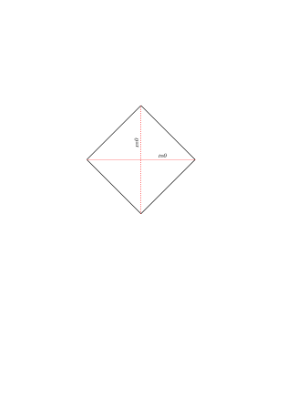
FIG. 1.: A conformal diagram of the constant $y$ and $z$ sections of the spacetime $M_{0}$. When the diagram is understood to depict $M_{0}$, each point in the diagram is a flat cylinder of circumference $2a$, coordinatized locally by $(y,z)$ with the identification $(y,z)\sim(y,z+2a)$. Because of the suppressed dimensions, the infinities of the diagram do not faithfully represent the infinity structure of $M_{0}$. The involution ${\tilde{J}}_{-}$ consists of the reflection $(t,x)\mapsto(t,-x)$ about the vertical axis, followed by the map $(y,z)\mapsto(-y,z+a)$ on the suppressed cylinder.

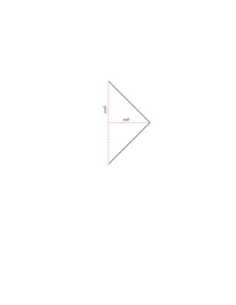
FIG. 2.: A conformal diagram of the constant $y$ and $z$ sections of the spacetime $M_{-}$. When the diagram is understood to depict $M_{-}$, the region $x>0$ is identical to that in the diagram of Figure 1, each point representing a suppressed cylinder. At $x=0$, each point in the diagram represents a suppressed open Möbius strip ($\simeq{{\mathbb{R}P}^{2}}\setminus\{\hbox{point}\}$), with the local coordinates $(y,z)$ identified by $(y,z)\sim(-y,z+a)$. Because of the suppressed dimensions, the infinities of the diagram do not faithfully represent the infinity structure of $M_{-}$.

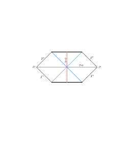
FIG. 3.: A conformal diagram of the Kruskal manifold. Each point represents a suppressed $S^{2}$ orbit of the ${\rm O}(3)$ isometry group. $(T,X)$ are the Kruskal coordinates introduced in subsection IV A, and the hypersurfaces $T=0$ and $X=0$ are shown. The involution $J^{L}$ (159) consists of the reflection $(T,X)\mapsto(T,-X)$ about the vertical axis, followed by the antipodal map $(\theta,\varphi)\mapsto(\pi-\theta,\varphi+\pi)$ on the suppressed two-sphere.

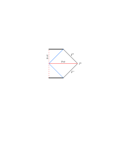
FIG. 4.: A conformal diagram of the ${{\mathbb{R}P}^{3}}$ geon [19]. Each point represents a suppressed orbit of the ${\rm O}(3)$ isometry group. The region $X>0$ is isometric to the region $X>0$ of the Kruskal spacetime, shown in figure 3; in particular, the ${\rm O}(3)$ isometry orbits in this region are two-spheres. At $X=0$, the ${\rm O}(3)$ orbits have topology ${{\mathbb{R}P}^{2}}$.

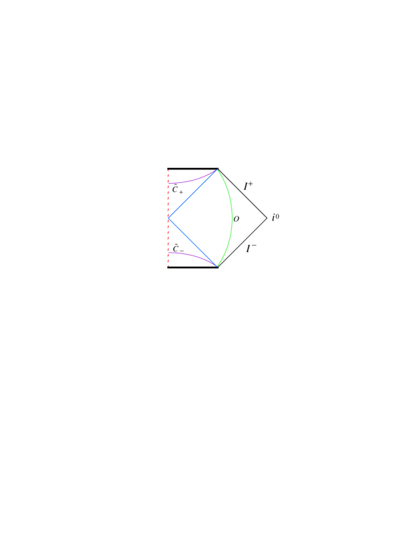
FIG. 5.: A conformal diagram for the emission and absorption calculation of subsection V D on the ${{\mathbb{R}P}^{3}}$ geon. The timelike hypersurface $O$ and the spacelike hypersurfaces ${\tilde{C}}_{+}$ and ${\tilde{C}}_{-}$ are shown. The diagram for the corresponding emission and absorption calculation on Kruskal is shown in Figure 3 of Ref. [6].

- [1] S. W. Hawking, Commun. Math. Phys. 43, 199 (1975).
- [2] J. M. Bardeen, B. Carter, and S. W. Hawking, Commun. Math. Phys. 31, 161 (1973).
- [3] J. D. Bekenstein, Nuovo Cimento Lett. 4, 737 (1972).
- [4] J. D. Bekenstein, Phys. Rev. D 9, 3292 (1974).
- [5] W. G. Unruh, Phys. Rev. D 14, 870 (1976).
- [6] J. B. Hartle and S. W. Hawking, Phys. Rev. D 13, 2188 (1976).
- [7] W. Israel, Phys. Lett. 57A, 107 (1976).
- [8] R. M. Wald, Quantum Field Theory in Curved Spacetime and Black Hole Thermodynamics (The University of Chicago Press, Chicago, 1994).
- [9] G. W. Gibbons and S. W. Hawking, Phys. Rev. D 15, 2752 (1977).
- [10] S. W. Hawking, in General Relativity: An Einstein Centenary Survey, edited by S. W. Hawking and W. Israel (Cambridge University Press, Cambridge, England, 1979).
- [11] D. N. Page, in Black Hole Physics, edited by V. D. Sabbata and Z. Zhang (Kluwer Academic Publishers, Dordrecht, 1992).
- [12] J. D. Brown and J. W. York, Phys. Rev. D 47, 1407 (1993).
- [13] J. D. Brown and J. W. York, Phys. Rev. D 47, 1420 (1993).
- [14] S. W. Hawking, G. T. Horowitz, and S. F. Ross, Phys. Rev. D 51, 4302 (1995). (gr-qc/9409013)
- [15] C. Teitelboim, Phys. Rev. D 51, 4315 (1995); Erratum, Phys. Rev. D 52, 6201 (1995). (hep-th/9410103)
- [16] J. I. Kapusta, Finite-temperature field theory (Cambridge University Press, Cambridge, England, 1989).
- [17] J. Polchinski, Rev. Mod. Phys. 68, 1245 (1996). (hep-th/9607050)
- [18] G. T. Horowitz, in Black Holes and Relativistic Stars, edited by R. M. Wald (The University of Chicago Press, Chicago, 1998). (gr-qc/9704072)
- [19] J. L. Friedman, K. Schleich, and D. M. Witt, Phys. Rev. Lett. 71, 1486 (1993); Erratum, Phys. Rev. Lett. 75, 1872 (1995). (gr-qc/9305017)
- [20] G. W. Gibbons, Nucl. Phys. B271, 497 (1986).
- [21] G. ’t Hooft, J. Geom. Phys. 1, 45 (1984).
- [22] D. Boulware, Phys. Rev. D 11, 1404 (1975).
- [23] S. A. Fulling, J. Phys. A 10, 917 (1977).
- [24] B. S. DeWitt, in General Relativity: An Einstein Centenary Survey, edited by S. W. Hawking and W. Israel (Cambridge University Press, Cambridge, England, 1979).
- [25] N. D. Birrell and P. C. W. Davies, Quantum Fields in Curved Space (Cambridge University Press, Cambridge, England, 1982).
- [26] S. Takagi, Prog. Theor. Phys. Suppl. 88, 1 (1986).
- [27] G. W. Gibbons, in Proceedings of the 10th Sorak School of Theoretical Physics, edited by J. E. Kim (World Scientific, Singapore, 1992).
- [28] A. Chamblin and G. W. Gibbons, Phys. Rev. D 55, 2177 (1996). (gr-qc/9607079)
- [29] R. Laflamme, Phys. Lett. 196B, 449 (1987).
- [30] J. A. Wolf, Spaces of Constant Curvature (McGraw-Hill, New York, 1967).
- [31] J. S. Dowker and R. Banach, J. Phys. A 11, 2255 (1978).
- [32] Handbook of Mathematical Functions, edited by M. Abramowitz and I. A. Stegun (Dover, New York, 1965).
- [33] Ref. [25], section 5.3.
- [34] M. Holschneider, Wavelets: An Analysis Tool (Clarendon Press, Oxford, 1995).
- [35] M. Ferraris and M. Francaviglia, Gen. Relativ. Gravit. 10, 283 (1979).
- [36] G. Arfken, Mathematical Methods for Physicists, second edition (Academic, New York, 1970).
- [37] A. Messiah, Quantum Mechanics (North-Holland, Amsterdam, 1991), Vol. I.
- [38] N. Dunford and J. S. Schwartz, Linear Operators (Interscience, New York, 1963), Vol. II.
- [39] S. M. Christensen and S. A. Fulling, Phys. Rev. D 15, 2088 (1977).
- [40] J. P. Boersma, Phys. Rev. D 55, 2174 (1997).
- [41] J. W. York, Phys. Rev. D 33, 2092 (1986).
- [42] B. F. Whiting and J. W. York, Phys. Rev. Lett. 61, 1336 (1988).
- [43] J. J. Halliwell and J. B. Hartle, Phys. Rev. D 41, 1815 (1990).
- [44] J. J. Halliwell and J. Louko, Phys. Rev. D 42, 3997 (1990).
- [45] B. L. Hu and A. Matacz, Phys. Rev. D 49, 6612 (1994). (gr-qc/9312035)
- [46] B. S. Kay and R. M. Wald, Phys. Rep. 207, 49 (1991).
- [47] K. Fredenhagen and R. Haag, Commun. Math. Phys. 127, 273 (1990).
- [48] R. Brandenberger and R. Kahn, Phys. Lett. 119B, 75 (1982).
- [49] K. Schleich and D. M. Witt, private communication.