Ringing the eigenmodes from compact manifolds

Abstract

We present a method for finding the eigenmodes of the Laplace operator acting on any compact manifold. The procedure can be used to simulate cosmic microwave background fluctuations in multi-connected cosmological models. Other applications include studies of chaotic mixing and quantum chaos.

1 Introduction

Much of physics boils down to solving differential equations subject to certain boundary conditions. Waves in a box are a classic example. The box we have in mind here is some closed manifold, and the waves are those of a massless scalar field. This picture arises naturally when studying density perturbations in a multi-connected universe[1]. The mathematical problem can be stated: Find all square integrable functions $\Psi_{q}({\bf x})$ that satisfy the partial differential equation

$$(\nabla+q^{2})\Psi_{q}({\bf x})=0\,.$$ (1)

Here $\nabla$ is the Laplace operator on some closed manifold $\Sigma$ and the constant $q$ is an eigenvalue of the Laplacian. The complexity of the problem is controlled by the geometry of $\Sigma$. When $\Sigma$ is $n$-dimensional Euclidean space, $E^{n}$, modulo some discrete group of covering transformations, $\Gamma$, it is a simple matter to write down analytic expressions for the eigenmodes $\Psi_{q}({\bf x})$. In contrast, if $\Sigma$ describes some compact hyperbolic manifold, $H^{n}/\Gamma$, then the eigenmodes cannot be expressed in closed analytic form. This difficulty is closely related to the chaotic behaviour of geodesic flows on compact negatively curved spaces[2]. Here we describe a numerical solution to the problem based on Fourier filtering solutions to the scalar wave equation $\Box\Psi=0$. While our approach works for any topology, we will focus on hyperbolic manifolds as these are of the most interest to cosmology.

2 Ringing out the modes

Rather than attack Laplace’s equation directly, we begin by introducing a ficticious time dimension $t$, thereby lifting the problem to solving the wave equation

$$\left({\partial^{2}\over\partial t^{2}}-\nabla\right)\Psi_{q}(t,{\bf x})=0\,,$$ (2)

on the Lorentzian manifold ${\cal M}=R\times\Sigma$. Consistent with this picture we adopt a product ansatz for the eigenmodes:

$$\Psi_{q}(t,{\bf x})=\exp(-i\omega_{q}t)\Psi_{q}({\bf x})\,.$$ (3)

The eigenfrequency $\omega_{q}$ is fixed by (2) to equal $q$. Assuming for now that the spatial boundary conditions have been properly enforced, we can evolve the initial data $\Psi(0,{\bf x})$, $\partial_{t}\Psi(t,{\bf x})|_{0}=0$ according to (2) to find $\Psi(t,{\bf x})$. By Fourier transforming in time:

$$a_{\omega}({\bf x})=\int_{0}^{\infty}\Psi(t,{\bf x})e^{i\omega t}dt\,,$$ (4)

and calculating the power spectrum

$$P(\omega)=\int_{\Sigma}|a_{\omega}|\,\sqrt{g}\,{d^{n}x}\,,$$ (5)

we are able to isolate the eigenfrequencies $\omega_{q}$. These are located at local maxima of $P(\omega)$. Once the eigenfrequencies are known the individual spatial eigenmodes can be extracted:

$$\Psi_{q}({\bf x})=\lim_{T\rightarrow\infty}{1\over T}\int_{0}^{T}\Psi(t,{\bf x})e^{iqt}dt\,.$$ (6)

In practice the integration time $T$ will be finite, so we can only resolve modes separated in frequency by at least $\Delta\omega=2\pi/T$.

The main difficulty in implementing the above procedure stems from the complicated periodic boundary conditions that are imposed by the topology. The remainder of this paper is devoted to describing a numerical solution to this problem, and illustrating how it works by finding the eigenmodes for a genus 2 surface with constant negative curvature.

3 The double doughnut

The manifold we will focus on is the two-hole doughnut $\Sigma=H^{2}/\Gamma$, where $\Gamma$ is a discrete subgroup of $SO(2,1)$ with presentation

$$\Gamma=\{g_{0},\,g_{1},\,g_{2},\,g_{3}\,:g_{0}g_{1}^{-1}g_{2}g_{3}^{-1}g_{0}^{-1}g_{1}g_{2}^{-1}g_{3}\}\,.$$ (7)

The group generators have the $SO(2,1)$ matrix representation[3]

$$g_{j}=R_{j}\left(\begin{array}[]{ccc}\cosh\eta&\sinh\eta&0\\ \sinh\eta&\cosh\eta&0\\ 0&0&1\end{array}\right)R_{j}^{-1}\,,$$ (8)

where $\eta=2\,{\rm arccosh}(1+\sqrt{2})$ and

$$R_{j}=\left(\begin{array}[]{ccc}1&0&0\\ 0&\cos(j\pi/4)&-\sin(j\pi/4)\\ 0&\sin(j\pi/4)&\cos(j\pi/4)\end{array}\right)\,.$$ (9)

The double doughnut can be obtained by gluing together opposite faces of a regular octagon with dihedral angles $\pi/4$. The octagonal fundamental domain (FD) is drawn in Fig. 1 using the Poincaré disc model for $H^{2}$.

Figure 1: The fundamental domain for the double doughnut (shown bordered by a solid line) in the Poincaré disk (bordered by a dashed line).

The double doughnut has area $4\pi$ and diameter $d=2\,{\rm arctanh}(2^{-1/4})\approx 2.448$. All distances are quoted in units of the curvature radius. The largest simply connected circle that can be drawn inside $\Sigma$ has radius $\eta_{-}={\rm arccosh}(1+\sqrt{2})$, and the smallest circle to fully enclose the fundamental domain has radius $\eta_{+}=2{\rm arccosh}(\sqrt{2+\sqrt{2}})$. The light crossing time varies in the interval $2\eta_{-}\leq t_{c}\leq 2\eta_{+}$, and has the mean value $t_{\lambda}=\sqrt{4\pi}\approx 3.545$. This is the Lyapunov time for chaotic flows on $\Sigma$, and represents the characteristic dynamical timescale for our system.

4 Solving the wave equation

The dynamics is described by a massless scalar field $\phi$ with action

$$S=\int\sqrt{-g}g^{\mu\nu}\partial_{\mu}\phi\partial_{\nu}\phi\,d^{3}x\,,$$ (10)

evolving on the Lorentzian manifold $(R\times\Sigma,g)$. Choosing a Poincaré metric for $H^{2}$ we have

$$ds^{2}=-dt^{2}+{4(dx^{2}+dy^{2})\over(1-x^{2}-y^{2})^{2}}\,.$$ (11)

The coordinate distance $r=(x^{2}+y^{2})^{1/2}$ is related to the proper distance $\eta$ by $r={\rm tanh}(\eta/2)$. To evolve the system numerically we begin by discretising time and space such that $x=i\,\Delta x$, $y=j\,\Delta y$ and $t=k\,\Delta t$. The discretised action then reads

$$S_{\Delta}= \sum_{i,j,k}\left[{(\phi(i+1,j,k)-\phi(i,j,k))^{2}\over\Delta x^{2}}+{(\phi(i,j+1,k)-\phi(i,j,k))^{2}\over\Delta y^{2}}\right.$$ (12)

$$\left.-{4\over(1-(i\Delta x)^{2}-(j\Delta y)^{2})^{2}}{(\phi(i,j,k+1)-\phi(i,j,k))^{2}\over\Delta t^{2}}\right]\Delta x\Delta y\Delta t\,.$$

The equations of motion that follow by varying $S_{\Delta}$ with respect to $\phi(i,j,k)$ are:

$$4\delta_{k}^{2}\phi(i,j,k)=(1-(i\Delta x)^{2}-(j\Delta y)^{2})^{2}\left[\delta_{i}^{2}\phi(i,j,k)+\delta_{j}^{2}\phi(i,j,k)\right]\,$$ (13)

where

$$\delta_{i}^{2}f(i)={f(i+1)-2f(i)+f(i-1)\over(\Delta x^{i})^{2}}\,.$$ (14)

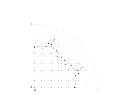
Figure 2: (a) The grid points are first sorted into masters (dark crosses), slaves (heavy dots) and freemen (light crosses). (b) The slave images (heavy dots) are located inside the FD.

Our next task is to enforce periodic boundary conditions at the edge of the fundamental domain. To do this we begin by sorting all points in the spatial grid into those inside and outside the fundamental domain. There is a simple sorting algorithm that works for all topologies. In what follows, $|{\bf x}|$ denotes the proper distance from the origin.

Algorithm 4.0. Point Sorting

1. If $|{\bf x}|<\eta_{-}$ then the point lies inside the FD. If $|{\bf x}|>\eta_{+}$ then the point lies outside the FD.

2. For $\eta_{-}<|{\bf x}|<\eta_{+}$, act on ${\bf x}$ by all $n$ group generators and their inverses to form the $2n$ image points ${\bf x}^{\prime}_{\pm}i=g_{i}^{\pm 1}{\bf x}$.

3. If $|{\bf x}^{\prime}_{\pm i}|<|{\bf x}|$ for any $i$, then ${\bf x}$ lies outside the fundamental domain, else ${\bf x}$ is inside the fundamental domain.

Only the “master” points inside the FD need to be evolved. However, forming the second derivatives $\delta_{i}^{2}\phi$ and $\delta_{j}^{2}\phi$ for the masters often requires knowledge of field values outside the FD. We refer to all points outside the FD that are within one grid point of a master as “slaves”. Points that are neither masters nor slaves play no part in the numerical evolution and are designated “freemen”. Each slave has a unique image inside the FD. We can find the position of these images using the following algorithm.

Algorithm 4.1. Locating the fundamental image

1. Act on ${\bf x}$ by all $n$ group generators and their inverses to form the $2n$ image points ${\bf x}^{\prime}_{\pm}i=g_{i}^{\pm 1}{\bf x}$.

2. Find the image point ${\bf x}^{\prime}_{\pm}i$ nearest the origin and call it ${\bf x}^{\prime}$.

3. If $|{\bf x}^{\prime}|<|{\bf x}|$ then let ${\bf x}={\bf x}^{\prime}$ and go to (i), else ${\bf x}$ is the fundamental image.

Since typical coordinate grids are not mapped into themselves by the fundamental group, the slave image points will not lie on the computational mesh. Therefore we have to interpolate to find the field value at each slave point. The procedure of point sorting and image finding is illustrated in Fig. 2. Only one quadrant of the FD is shown since the FD has 8-fold symmetry. The slave images are those of slave points located in the other three quadrants.

Figure 3: Interpolating the image of a slave point.

The interpolation of the slave values is done using either a 3-point, 4-point or 6-point interpolation scheme. Employing the labelling convention shown in Fig. 3, the 6-point interpolation is described by

$$\phi(p\,\Delta x,q\,\Delta y)= q(q-1)/2\,\phi_{0-1}+p(p-1)/2\,\phi_{-10}$$ (15)

$$+(1-pq-p^{2}-q^{2})\phi_{00}+p(p-2q+1)/2\,\phi_{10}$$

$$+q(q-2p+1)/2\,\phi_{01}+pq\phi_{11}+{\cal O}(\epsilon^{3}\phi_{00})\,.$$

Here $\epsilon={\rm max}(\Delta x,\Delta y)$. By rotating the coordinates so that the interpolation is performed in the quadrant $x>0,\,y>0$, we can ensure that the $(0,0)$ vertex of the cell enclosing the image point lies nearest the origin. This increases the chances that $(-1,0)$ and $(0,-1)$ are master points. Nevertheless, we need to check that all points involved in the interpolation are either masters or slaves. If a freeman is used in the interpolation it must be enslaved. Once this is done for all the slave points we arrive at a set of $N$ coupled linear equations involving $N$ slaves and $M$ masters (the slave drivers). Writing the list of slaves and slave drivers as the column vectors $\phi_{S}$ and $\phi_{SD}$, the interpolation equation (15) can be used to form the linear system

$$A\phi_{S}=B\phi_{SD}\,\quad\Rightarrow\quad\phi_{S}=A^{-1}B\phi_{SD}\,,$$ (16)

where $A$ is a $N\times N$ matrix and $B$ is a $N\times M$ matrix. This procedure only has to be performed once at the beginning of a simulation. The $N\times M$ matrix $C=A^{-1}B$ can then be stored and called during the numerical evolution. In summary, at each time step the masters are evolved according to (13). The slaves are then updated using (16). The slaves are the glue that holds together identified sides of the fundamental cell. If the glue is poor energy can either leak in or out of the system. Thus, by keeping track of the total energy $E=K+G$ we can check that the periodic boundary conditions are being properly implemented. The kinetic energy is given by

$$K_{k}=\sum_{i,j}^{\rm masters}\left[{4(\phi(i,j,k)-\phi(i,j,k-1))^{2}\over(1-(i\Delta x)^{2}-(j\Delta y)^{2})^{2}\Delta t^{2}}\right]\Delta x\Delta y\,.$$ (17)

and the gradient energy is given by

$$G_{k}=\sum_{i,j}^{\rm masters}\left[{(\phi(i+1,j,k)-\phi(i,j,k))^{2}\over\Delta x^{2}}+{(\phi(i,j+1,k)-\phi(i,j,k))^{2}\over\Delta y^{2}}\right]\Delta x\Delta y,$$ (18)

5 Results

Several simulations were run using $301^{2}$ grids covering the region $-0.8<x,y<0.8$. The coordinate grid spacings were: $\Delta x=\Delta y=2/375$ and $\Delta t=\Delta x/10$. The proper distance between grid points varies between $\delta x=\Delta x$ near the origin and $\delta x=(2+\sqrt{2})\Delta x$ at the extremities of the FD. Consequently, the resolution is $\sim 3.4$ times worse at the edge of the FD. Other metrics could be used to give a more even coverage if desired. As a check on the accuracy of the code the area was evaluated and compare to the continuum answer:

$$A=\sum_{i,j}^{{\rm masters}}{4\Delta x\Delta y\over(1-(i\Delta x)^{2}-(j\Delta y)^{2})^{2}}=(1.00014)\,4\pi\,.$$ (19)

Two types of initial conditions were used for $\phi(0,{\bf x})$. The first employed a random superposition of Gaussian peaks and was designed to excite as many eigenmodes as possible. The second employed a superposition of two spherically symmetric eigenmodes ($q=0.1$ and $q=0.5$) of the Laplacian on $H^{2}$. This choice was designed to excite low lying eigenmodes. The waveforms were smoothed to remove any large gradients caused by the imposition of the periodic boundary conditions. The residual monopole contribution was removed to increase our chances of resolving any low lying multipoles. A stroboscopic sequence showing the evolution of the random Gaussian peaks is shown in Fig. 4.

The wave was evolved for $2^{17}$ timesteps, which equates to $T=69.9051$ curvature units, or roughly 20 light crossing times. The total energy remained roughly constant throughout the simulation, although there were $\sim\pm 2\%$ fluctuations about the mean value. We believe these variations are due to the uneven grid resolution.

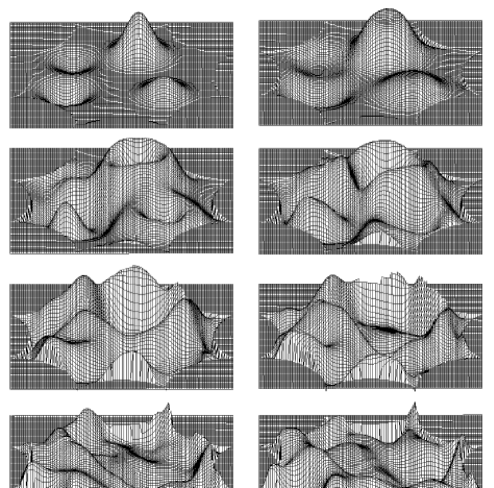
Figure 4: The evolution of an initially static waveform shown every 0.2 time units. Time runs cartoon style.

The wave was Fourier analysed to produce the scaled power spectrum shown in Fig. 5. The power spectrum is multiplied by $\sqrt{\omega}$ for $\omega>0$ to reflect the larger statistical weight of the high frequency modes.

Figure 5: The scaled power spectrum for the wave shown in Fig. 4.

The first three peaks are at $\omega_{1}=q_{1}=1.97\pm 0.09$, $q_{2}=2.30\pm 0.09$ and $q_{3}=2.90\pm 0.09$. The errors reflect the finite frequency resolution of $\Delta\omega=2\pi/T=0.09$. Aside from some residual monopole power at $q=0$ there is no evidence for any low lying eigenmodes. We will return to this crucially important point later.

Figure 6: The two lowest eigenmodes found by Fourier filtering.

By Fourier filtering at $\omega=\omega_{1}$ and $\omega=\omega_{2}$ we are able to extract the corresponding spatial eigenmodes. These are displayed in Fig. 6. By numerically evaluating the Laplacian of these waveforms we were able to confirm that they are indeed eigenmodes with the correct eigenvalues. We illustrate this in Fig. 7 by displaying the eigenmode $\phi_{q_{3}}({\bf x})$ and $-q_{3}^{-2}\nabla\phi_{q_{3}}({\bf x})$. The agreement is remarkably good over most of the FD, save for some small regions where the spatial gradients are large. The eigenmodes can be improved by a second scrubbing run. To do this we use the approximate eigenmode as initial data and evolve the system as before while filtering at the appropriate eigenfrequency. This helps to remove contamination from the other eigenmodes.

Figure 7: (a) The $q_{3}$ eigenmode. (b) The $q_{3}$ eigenmode acted on by $-q^{-2}_{3}\nabla$.

One possible explanation for the lack of eigenmodes below $q_{1}=1.97$ might be a lack of long range power in our choice of initial conditions. To check this we tried a different initial waveform based on a superposition of the spherically symmetric $q=0.1$ and $q=0.5$ eigenmodes of $H^{2}$. When the periodic boundary conditions are imposed the resulting initial waveform has 8-fold symmetry.

Figure 8: The 8-fold symmetric $q=0.1,0.5$ initial waveform and the resulting scaled power spectrum.

The scaled power spectrum shown in Fig. 8 shows no sign of any modes below $q_{1}=1.97$. As expected, many of the modes excited by the random superposition of Gaussian peaks are missing from the spectrum produced by the 8-fold symmetric initial conditions. However, the modes that are present agree with those in seen in Fig. 5.

6 Supercurvature modes

In $n$ dimensions the eigenmode spectrum for $H^{n}$ takes all values in the range $q=[q_{0},\infty)$, where $q_{0}=(n-1)/2$. Modes with $q<q_{0}$ are not square integrable in infinite $n$-dimensional hyperbolic space, but they are square integrable in the compact quotients $\Sigma^{n}=H^{n}/\Gamma$. According to Buser[5], many compact hyperbolic manifolds support supercurvature modes with $q<q_{0}$. The name supercurvature refers to the fact that these modes support significant long range correlations on scales larger than the curvature scale. In contrast, modes with $q>q_{0}$ have exponentially damped correlations outside the curvature radius, even though their wavelengths $\lambda=2\pi(q^{2}-q_{0}^{2})^{-1/2}$ may greatly exceed the curvature scale. This suppression can be understood on the grounds of flux conservation in a space where the volume grows exponentially on large scales. Supercurvature modes are very important in a cosmological setting as even a single supercurvature mode can significantly increase the amplitude of cosmic microwave background fluctuations on large angular scales[4].

There are a number of upper and lower bounds for the lowest eigenvalue, $q_{1}>q_{0}$, of the Laplacian on $H^{n}/\Gamma$. In two dimensions the tightest upper bound we know of was found by Cheng[6]:

$$q_{1}^{2}\leq{1\over 4}+\left({2\pi\over d}\right)^{2}\,,$$ (20)

where $d$ is the diameter of $\Sigma$. Applying this to our genus 2 example we find that $q_{1}\leq 2.61$, which is consistent with what we found ($q_{1}=1.97\pm 0.09$). Using Cheeger’s inequality, $q_{1}^{2}\geq h^{2}/4$, where $h$ is Cheeger’s isoperimetric constant, Balazs & Voros[3] suggest that $q_{1}\geq 0.7$. This is also consistent with our result.

To be certain that we have not missed any low lying eigenvalues we need to use other methods such as the Selberg-Gutzwiller global eigenvalue count[7]. After presenting our results in Cleveland, we discovered a paper by Aurich & Steiner[8] that calculates all the low lying eigenvalues for the double doughnut using a suitably regularised Gutzwiller trace formula. They find the lowest three eigenvalues to be $q_{1}=1.959$, $q_{2}=2.314$ and $q_{3}=2.872$, in perfect agreement with our values. This proves that we did not miss any low lying eigenvalues. While their values are sharper, the advantage of our method is that it allows us to extract the eigenmodes in addition to the eigenvalues.

The lack of low lying eigenmodes on the regular octagon is probably related to its high degree of symmetry. Indeed, it is possible to move to an alternative description of the manifold using a larger fundamental group and a fundamental cell $96$ times smaller than the octagon[3]. Viewed from this perspective, the lowest eigenmode is remarkably low, as it corresponds to a wave with a wavelength $\sim 10$ times larger than the diameter of the desymmetrised fundamental cell.

7 Concluding Remarks

Having demonstrated that our approach works in 2-dimensions, our next task is to apply it to the cosmologically relevant case where $\Sigma$ is a compact hyperbolic 3-manifold. The computational cost of having an extra dimension will be offset by the availability of examples with very small fundamental domains. Many small hyperbolic 3-manifolds have FD’s that have outradii, $\eta_{+}$, smaller than the radius of curvature[9]. Consequently, space looks approximately Euclidean inside the FD, so standard coordinate systems such as the Klein metric will produce fairly uniform computational grids. Once we have found all the low lying eigenmodes we can use them to produce simulated maps of the cosmic microwave background radiation. These maps can then be compared to observational data, or used to test proposals for finding the large scale topology of the universe[10].

References

References

- [1] M. Lachieze-Rey & J-P. Luminet, Phys. Rep. 254, 135 (1995).
- [2] M.V. Berry, J. Phys. A10, 2083 (1977); M.V. Berry, N. L. Balazs, M. Tabor & A. Voros, Ann. Phys. N.Y. 122, 26 (1979).
- [3] N.L. Balazs and A. Voros, Phys. Rep. 143, 109 (1986).
- [4] J. Garcia-Bellido, Phys. Rev. D54, 2473, (1996).
- [5] P. Buser, in Geometry of the Laplace Operator, Proc. Symp. Pure Math. XXXVI, Am. Math. Soc. (1980).
- [6] S.-Y. Cheng, Math. Z. 143, 289 (1975).
- [7] M.C. Gutzwiller, J. Math. Phys. 11, 1791 (1970); ibid 12, 343 (1971).
- [8] R. Aurich & F. Steiner, Physica D 39, 169, (1989).
- [9] J. Weeks, SnapPea: A computer program for creating and studying hyperbolic 3-manifolds, available at http://www.geom.umn.edu:80/software.
- [10] N.J. Cornish, D. Spergel & G. Starkman, in this volume, Class. Quant. Grav. (1998); J. Weeks, in this volume, Class. Quant. Grav. (1998); J. J. Levin, in this volume, Class. Quant. Grav. (1998).