Scaling of curvature in sub-critical gravitational collapse

Abstract

We perform numerical simulations of the gravitational collapse of a spherically symmetric scalar field. For those data that just barely do not form black holes we find the maximum curvature at the position of the central observer. We find a scaling relation between this maximum curvature and distance from the critical solution. The scaling relation is analogous to that found by Choptuik for black hole mass for those data that do collapse to form black holes. We also find a periodic wiggle in the scaling exponent.

PACS 04.20.-q, 04.20.Fy, 04.40.-b

I Introduction

Choptuik has found scaling phenomena in gravitational collapse.[1] He numerically evolves a one parameter family of initial data for a spherically symmetric scalar field coupled to gravity. Some of the data collapse to form black holes while others do not. There is a critical value of the parameter separating those data that form black holes from those that do not. The critical solution (the one corresponding to the critical parameter) has the property of periodic self similarity: after a certain amount of logarithmic time the profile of the scalar field repeats itself with its spatial scale shrunk. For parameters slightly above the critical parameter the mass of the black hole formed scales like ${(p-p*)}^{\gamma}$ where $p$ is the parameter, $p*$ is its critical value and $\gamma$ is a universal scaling exponent that does not depend on which family is being evolved. Numerical simulations of the critical gravitational collapse of other types of spherically symmetric matter were subsequently performed. These include complex scalar fields [2], perfect fluids [3], axions and dilatons [4], and Yang-Mills fields [5]. In addition scaling has been found in the collapse of axisymmetric gravity waves [6], and in a perturbative analysis of fluid collapse with no symmetries[7]. Thus scaling seems to be a generic feature of critical gravitational collapse. In some of these systems the critical solution has periodic self-similarity while in other systems it has exact self-similarity.

These phenomena were discovered numerically, so one would like to have an analytic explanation for why systems that just barely undergo gravitational collapse behave in this way. An explanation of the scaling of black hole mass was provided by Koike, Hara and Adachi [8]. These authors assume that the critical solution is exactly self-similar and has exactly one unstable mode. Exact self-similarity means that the critical solution has a homothetic Killing vector, i.e. a vector field $\xi$ such that ${{\cal L}_{\xi}}{g_{ab}}=-\,2\,{g_{ab}}$. Let coordinates be chosen so that ${\xi}=\partial/\partial t$. Then the unstable mode grows as $e^{\kappa t}$ for some constant $\kappa$. The result of reference[8] is that black hole mass scales as ${(p-p*)}^{\gamma}$ where $\gamma=1/\kappa$.

The results of reference[8] were extended to the case of periodic self-similarity by Gundlach[9] and by Hod and Piran [10]. Here, the assumptions are that the critical solution is periodically self-similar and has exactly one unstable mode. Periodic self-similarity means that there is a diffeomorphism $\zeta$ and a number $\Delta$ such that ${\zeta^{*}}({g_{ab}})={e^{-2\Delta}}\,{g_{ab}}$. Let coordinates be chosen so that $\zeta$ is the transformation $t\to t+\Delta$ with the other coordinates remaining constant. Then the unstable mode grows as $e^{\kappa t}$ multiplied by a function that is periodic in $t$. (Here again $\kappa$ is a constant). The result is still a scaling relation for black hole mass; but it is more complicated than a linear relation. A graph of $\ln M$ vs. $\ln(p-p*)$ is no longer a straight line; but is instead the sum of a linear function and a periodic function. The slope of the linear function is again $\gamma=1/\kappa$ and the period of the periodic function is $\Delta/(2\gamma)$. The scaling relation for black hole mass in scalar field collapse was originally thought to be linear[1] because the additonal “wiggle” is small. This small wiggle was found numerically by Hod and Piran[10].

Any proposed analytic explanation of a numerically observed phenomenon needs to be tested. Perhaps the best such test is to ask what other phenomena are predicted by the explanation and then to see whether those phenomena occur. One remarkable property of the derivations in references[8, 9, 10] is their generality. The only property of black hole mass that is used is that it is a global property of the spacetime and has dimensions of length. Furthermore, the derivations apply as well to solutions that do not collapse to form black holes as to those that do: the only assumption needed is that the initial data be near data that leads to the critical solution.

Therefore, it is a consequence of the explanation of references[8, 9, 10] that other scaling relations exist in near-critical collapse, even in the case where no black hole forms. This is in contrast to the case of phase transitions, where scaling behavior occurs only on one side of the critical parameter. For the case of a periodically self-similar critical solution, the scaling relation should have a wiggle with period $\Delta/(2\gamma)$. For the case where no black hole forms, the field collapses for a while and then disperses. Therefore, at the position of the central observer, the scalar curvature should grow, achieve some maximum value $R_{\rm max}$ and then approach zero at late times. This $R_{\rm max}$ is a characteristic of the spacetime and has dimensions of ${\rm length}^{-2}$. Therefore, one would expect that a graph of $\ln{R_{\rm max}}$ vs. $\ln(p*-p)$ should be a curve with average slope $-\,2\gamma$ (where $\gamma$ is the same constant that occurs in the black hole mass scaling relation) and a wiggle with period $\Delta/(2\gamma)$.

In order to test the explanation of references[8, 9, 10], this paper presents the results of numerical investigations which explore whether $R_{\rm max}$ obeys exactly this sort of scaling relation. We have performed numerical simulations of the collapse of a family of initial data for a spherically symmetric scalar field. The data were chosen to be near the critical solution, but with $p<p*$ so that no black hole forms. For each evolved spacetime in the family we find $R_{\rm max}$, the maximum scalar curvature at the central observer. We then plot $\ln{R_{\rm max}}$ vs $\ln(p*-p)$ and show that the resulting curve is a straight line with a periodic wiggle, where the slope of the line is $-\,2\gamma$ and the period of the wiggle is $\Delta/(2\gamma)$. Section II briefly presents the numerical method used. The results are presented in Section III. Section IV contains a discussion of some of the implications of the results of these studies.

II Numerical method

The numerical method used is that of Garfinkle[11]. This method is a modification of an earlier method due to Goldwirth and Piran[12], which is in turn based on analytical work by Christodoulou [13]. The matter is a massless, minimally coupled scalar field, with both scalar field and metric spherically symmetric. In addition to the usual area coordinate $r$ and angular coordinates, we use a null coordinate $u$ defined to be constant along outgoing light rays, and equal to proper time of the central observer at $r=0$. Instead of directly using the matter field $\phi$, it is convenient to work with the quantity $h\equiv(\partial/\partial r)(r\phi)$. Due to the spherical symmetry, the metric is completely determined by the matter. This is made explicit as follows: for any function $f(u,r)$ define

$${\bar{f}}(u,r)\equiv{1\over r}\;{\int_{0}^{r}}\;f(u,{\tilde{r}})\;d{\tilde{r}}\;\;\;.$$

Then define the quantity $g$ by

$$g(u,r)\equiv\exp\left(4\pi\;{\int_{0}^{r}}\;{{d{\tilde{r}}}\over{\tilde{r}}}\;{{\left[h(u,{\tilde{r}})-{\bar{h}}(u,{\tilde{r}})\right]}^{2}}\right)\;\;\;.$$

Then the metric is given by

$$d{s^{2}}=-\,g\,du\,({\bar{g}}\,du\,+\,2\,dr)\;+\;{r^{2}}\,d{\Omega^{2}}$$

where $d{\Omega^{2}}$ is the usual unit two-sphere metric. Define the operator

$$D\equiv{\partial\over{\partial u}}\;-\;{1\over 2}\;{\bar{g}}\;{\partial\over{\partial r}}\;\;\;.$$

$D$ is essentially the derivative operator along ingoing light rays. The evolution equation for $h$ is

$$D\,h={1\over{2r}}\;(g-{\bar{g}})(h-{\bar{h}})\;\;\;.$$

The numerical treatment of these equations is as follows: given $h$ at some time $u$, the quantities ${\bar{h}},\,g$ and $\bar{g}$ are evaluated in turn, with the integrations done using Simpson’s rule. This is quite accurate, except near $r=0$. For the region near $r=0$ we use a Taylor series method: first we fit the values of $h$ near $r=0$ to a straight line and thus evaluate the quantity

$${h_{1}}\equiv{{\left.{{\partial h}\over{\partial r}}\right|}_{r=0}}\;\;\;.$$

Near $r=0$ the quantities ${\bar{h}},\,g$ and $\bar{g}$ are then given by

$${\bar{h}}=h\;-\;{1\over 2}\;{h_{1}}\,r\;+\;O({r^{2}})\;\;\;,$$

$$g=1\;+\;{\pi\over 2}\;{h_{1}^{2}}\,{r^{2}}\;+\;O({r^{3}})\;\;\;,$$

$${\bar{g}}=1\;+\;{\pi\over 6}\;{h_{1}^{2}}\,{r^{2}}\;+\;O({r^{3}})\;\;\;.$$

(Note: equations (8) and (9) correct an error in reference[11]). The value of the scalar curvature at $r=0$ is given by

$$R(u,0)=-\,2\pi\,{h_{1}^{2}}\;\;\;.$$

Equation (5) can be regarded as a set of decoupled ODEs for the value of $h$ along each ingoing light ray. These equations are used to determine the evolution of $h$ for one time step, and then the whole process is continued until the scalar field either forms a black hole or disperses. The critical solution is found by a binary search of $p$ parameter space to find the boundary between those data that form black holes and those that do not. Since $h$ is evolved along ingoing light rays, the spatial scale of the grid shrinks as the evolution proceeds. With the outermost gridpoint chosen to be the light ray that hits the singularity of the critical solution, the grid shrinks at the same rate as the spatial features of the scalar field. These features are therefore resolved throughout the evolution.

III Results

All runs were done with 300 spatial gridpoints. The code was run in quadruple precision on Dec alpha workstations and in double precision on a Cray YMP8. The initial data for the scalar field was chosen to be of the form

$$\phi(0,r)=p\;{r^{2}}\;\exp\left[{{(r-{r_{0}})}^{2}}/{\sigma^{2}}\right]\;\;\;.$$

Here $p$ is our parameter, and $r_{0}$ and $\sigma$ are constants. This is the family which was evolved in [11], where the value of the critical parameter $p*$ was found. Here we evolve this family for 100 values of $p<p*$, chosen equally spaced in $\ln(p*-p)$. During each evolution, we keep track of the behavior of the scalar curvature at $r=0$ and thus find the maximum of its absolute value $R_{\rm max}$.

Figure 1 shows a graph of $\ln{R_{\rm max}}$ vs. $\ln(p*-p)$. In the figure, each point is the result of one evolution. The points were fit to a five parameter curve that is a straight line plus a sine wave. (Both the figures and the curve fitting were done with KaleidaGraph). Figure 1 also shows this curve. However, because of the large number of data points and the goodness of the fit, the curve is indistinguishable from the data points.

The parameters of the fit are the slope and intercept of the line, and the amplitude, period and phase of the sine wave. To examine the goodness of the fit, the data and the fit are plotted in Figure 2 with the straight line piece of the fit subtracted from both of them. Here, we see that the fit is good, but not exact. Indeed there is no reason for the fit to be exact: the function should be periodic with period $\Delta/(2\gamma)$ and therefore a sum of sine waves of period $\Delta/(2\gamma n)$ for integer $n$. In addition, inaccuracies in the numerical evolution of the spacetime contribute some “noise” to the data points.

Of particular interest are the slope of the line and the period of the sine wave. It is not clear what error should be attributed to the parameters of the fit. While there is an error that can be obtained formally from the fitting process, there may be additional errors due to inaccuracies of the numerical evolution algorithm itself. Using three significant figures, we find that the slope of the line is -0.747 and the period of the sine wave is 4.63. The values of $\gamma$ and $\Delta$ given in reference[9] are $\gamma=0.374\pm 0.001$ and $\Delta=3.4453\pm 0.0005$. These numbers give rise to $-\,2\gamma=-0.748\pm 0.002$ and $\Delta/(2\gamma)=4.61\pm 0.01$. Thus it is clear that the slope of the line is $-2\,\gamma$ and the period of the sine wave is $\Delta/(2\gamma)$. That is, as expected, $R_{\rm max}$ scales like ${(p*-p)}^{-2\gamma}$ with a periodic wiggle of period $\Delta/(2\gamma)$.

IV Discussion

Our paper considers the behavior of only one sort of curvature: scalar curvature at the position of the central observer. Clearly there are other sorts of curvature that one could treat. The quantities ${{|{R^{ab}}{R_{ab}}|}^{1/2}}$ and ${{|{R^{abcd}}{R_{abcd}}|}^{1/2}}$ would also be expected to scale like ${(p*-p)}^{-2\gamma}$. In the case of spherical symmetry, and evaluated on the world line of the central observer, these quantities yield nothing new. All of them are proportional to $h_{1}^{2}$. This is what one would expect, since in spherical symmetry the gravitational field has no degrees of freedom of its own, and the Ricci tensor just depends quadratically on the gradient of the scalar field. However, there is no need to restrict consideration to the world line of the central observer. One could also consider the maximum value of the scalar curvature (or any of these other curvatures) over the whole spacetime. In this project we chose the world line of the central observer mostly for convenience, since it is very easy to evaluate the scalar curvature there. We do not expect the results to differ much if instead we find the maximum of the scalar curvature over the whole spacetime, since in a spherically symmetric collapse we would expect the spacetime maximum of the scalar curvature to occur at or near the world line of the central observer.

The situation is different in the case of collapse without spherical symmetry. Here there is no central observer and so the spacetime maximum of curvature is the appropriate quantity to consider. (Though in the case of axisymmetry with equatorial plane reflection symmetry there is a preferred observer). Choptuik scaling has been shown to occur in the collapse of vacuum, axisymmetric gravity waves [6]. It would be interesting to see whether curvature scaling takes place in this situation. Of course, since the spacetimes are vacuum, $R$ and ${R^{ab}}{R_{ab}}$ vanish. Therefore, the appropriate quantity to consider is the spacetime maximum of ${{|{R^{abcd}}{R_{abcd}}|}^{1/2}}$. We would expect this quantity to scale like ${{(p*-p)}^{-2\gamma}}$ (with a small periodic wiggle) for those spacetimes that just barely do not collapse to form black holes. It would also be of interest to investigate the gravitational collapse of an axisymmetric scalar field and look for scaling in the spacetime maxima of $R$ and ${|{R^{ab}}{R_{ab}}|}^{1/2}$ as well as ${{|{R^{abcd}}{R_{abcd}}|}^{1/2}}$.

Although we would expect that a quantity with dimensions of length would scale as ${{|p-p*|}^{\gamma}}$, it is known that in some cases this does not occur. Hod and Piran[14] have performed a numerical simulation of the collapse of a spherically symmetric charged scalar field. Here the black holes formed have charge as well as mass. Since charge has units of length, one might expect that near the critical solution charge scales as ${{(p-p*)}^{\gamma}}$. Instead, the charge vanishes faster: like ${{(p-p*)}^{2\gamma}}$. (This scaling is explained in references [14, 15]). Thus a simple consideration of the dimensions of a quantity is not sufficient, in all cases, to predict the scaling of that quantity. It would be interesting to know which quantities can be expected to scale as their dimensions would suggest, and which behave anomalously. In any case, some sort of scaling behavior can be expected for many different quantities, both in spacetimes that barely form black holes and in those that barely do not.

V Acknowledgements

This work was partially supported by NSF grant PHY-9722039 and by a Cottrell College Science Award of Research Corporation to Oakland University. Some of the computations were performed at the Ohio Supercomputer Center.

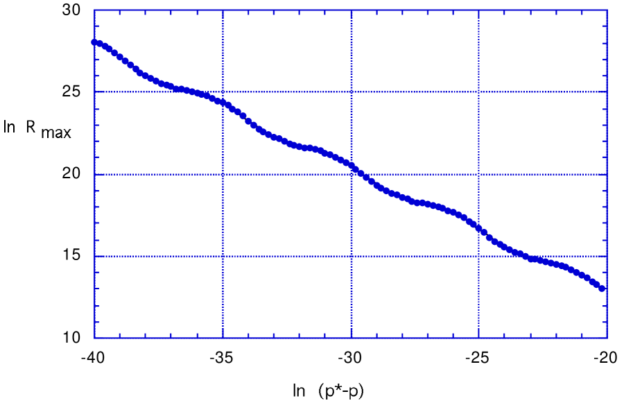
FIG. 1.: $\ln{R_{\rm max}}$ is plotted vs. $\ln(p*-p)$. The result is a line with slope $-2\gamma$ and a periodic wiggle with period $\Delta/(2\gamma)$

FIG. 2.: The data and the fitted curve of figure 1 are plotted with the straight line piece of the fitted curve removed from both.

REFERENCES

- [1] M. Choptuik, Phys. Rev. Lett. 70, 9 (1993)
- [2] E.W. Hirschmann and D.M. Eardley, Phys. Rev. D51, 4198 (1995)
- [3] C.R. Evans and J.S. Coleman, Phys. Rev. Lett. 72, 1782 (1994)
- [4] R.S. Hamade, J.H. Horne and J.M. Stewart, Class. Quantum Grav. 13, 2241 (1996)
- [5] M. Choptuik, T. Chmaj and P. Bizon, Phys. Rev. Lett. 77, 424 (1996)
- [6] A.M. Abrahams and C.R. Evans, Phys. Rev. Lett. 70, 2980 (1993)
- [7] C. Gundlach, gr-qc/9710066
- [8] T. Koike, T. Hara and S. Adachi, Phys. Rev. Lett. 74, 5170 (1995), T. Hara, T. Koike and S. Adachi, gr-qc/9607010
- [9] C. Gundlach, Phys. Rev. D55, 695 (1997)
- [10] S. Hod and T. Piran, Phys. Rev. D55, 440 (1997)
- [11] D. Garfinkle, Phys. Rev. D51, 5558 (1995)
- [12] D.S. Goldwirth and T. Piran, Phys. Rev. D36, 3575 (1987)
- [13] D. Christodoulou, Commun. Math. Phys. 105, 337 (1986)
- [14] S. Hod and T. Piran, Phys. Rev. D55, 3485 (1997)
- [15] C. Gundlach and J. Martin-Garcia, Phys. Rev. D54, 7353 (1996)