Gravitational evolution and stability of boson halos

Abstract

We investigate the gravitational evolution of dark matter halos made up of a massless bosonic field. The coupled Einstein-Klein-Gordon equations are solved numerically, showing that such a boson halo is stable and can be formed under a large class of initial conditions. We also present an analytical proof that such objects are stable in the Newtonian limit. In the context of boson stars made of massive scalar fields, we introduce new solutions with an oscillatory scalar field, similar to boson halos. We find that these solutions are unstable.

I Introduction

Boson stars are self-gravitating configurations which are described mathematically by the Einstein-Klein-Gordon equations [1]. In order to find such globally regular solutions it is necessary to have a conserved particle number which is fulfilled if one uses a complex scalar field and a potential with global $U(1)$ symmetry. Investigations so far have shown that stable and unstable configurations exist so that study to a greater extent makes sense [2, 3, 4]. A boson star can have values of the mass over large orders of magnitudes; it depends on the mass of the scalar field and possible self-interactions [5]. A recent paper described the effects if the scalar field would interact only gravitationally so that the star is transparently similar as a dark matter halo of a galaxy [6]. Baryonic matter could then move within the gravitational potential of the star and if perhaps a accretion disk can be built the radiation would suffer a gravitational redshift. Redshift of an iron-K line is actually observed within the center of a Seyfert galaxy [7].

Boson star solutions are characterized by an exponential decrease of the scalar field for which a mass term in the potential is responsible. A zero temperature solution is usually considered in which all scalar particles are within the same ground state forming a Bose-Einstein condensate. The size of this general-relativistic object is given by the Compton wavelength. If one ‘switches off’ the mass of the scalar field, the Compton wavelength is infinite. Then the massless scalar particles are within a coherent state, a kind of ‘boson star’, which in principle has an infinite range. Investigations of these solutions [8, 9, 10, 11] which we call now boson halos, have shown that the mass of these objects increases linearly, a behavior suggested by HI observations for spiral and dwarf galaxies. It was shown that the rotation curves for galaxies could be very well fitted by this kind of matter. In this paper, we present an analytical proof showing the stability of the Newtonian solutions.

In this paper we also examine numerically how these objects could have formed and show that they are stable. For this purpose, we use the process of gravitational cooling as described in [12]. We add a small radial perturbation to a solution and show that the evolved solution does not disperse or form a black hole, hence it is stable. Furthermore, we present here for the first time solutions with an oscillating scalar field for the massive case; we find that they are unstable.

In section II we present the mathematical foundations of the problem of bosonic objects made from massless scalar fields. We set up equilibrium equations and approximate solutions. We then set up the evolution equations which we use in our code. In section III we discuss our numerical studies on the formation of scalar halos followed in section IV by an analytical proof of stability of these objects. In section V we discuss our numerical studies of stability of bosonic halos. In section VI we discuss new oscillatory (in space) solutions for massive scalar fields. Finally we have a discussion of our results and their implications in section VII.

II Mathematical Foundations of the Problem

In this Section we start with the Lagrangian for the system and set up the equilibrium equations and their solutions as well as the evolution equations with which we evolve the equilibrium solutions.

A Einstein-scalar-field equations

The Lagrange density of a complex self-gravitating scalar field reads

$${\cal L}=\frac{1}{2}\sqrt{\mid g\mid}\left[\frac{1}{\kappa}R+g^{\mu\nu}(\partial_{\mu}\Phi^{\ast})(\partial_{\nu}\Phi)-U(|\Phi|^{2})\right]\;,$$ (1)

where $R$ is the curvature scalar, $\kappa=8\pi G$, $G$ the gravitation constant ($\hbar=c=1$), $g$ the determinant of the metric $g_{\mu\nu}$, $\Phi$ the complex scalar field, and $U$ the potential depending on $|\Phi|^{2}$ so that a global $U(1)$ symmetry is conserved. Then we find the coupled system

$$R_{\mu\nu}-\frac{1}{2}g_{\mu\nu}R = -\kappa T_{\mu\nu}(\Phi)\;,$$ (2)

$$\Box\Phi+\frac{\partial U}{\partial\Phi^{\ast}} = 0\;,$$ (3)

where

$$T_{\mu\nu}=(\partial_{\mu}\Phi^{\ast})(\partial_{\nu}\Phi)-\frac{1}{2}g_{\mu\nu}[g^{\sigma\kappa}(\partial_{\sigma}\Phi^{\ast})(\partial_{\kappa}\Phi)-U(|\Phi|^{2})]$$ (4)

is the energy-momentum tensor and

$$\Box=\partial_{\mu}\Bigl{[}\sqrt{\mid g\mid}g^{\mu\nu}\partial_{\nu}\Bigr{]}/\sqrt{\mid g\mid}$$ (5)

the generally covariant d’Alembertian.

For spherically symmetric solutions we use the following line element

$$ds^{2}=N^{2}({\bf r},{\bf t})d{\bf t}^{2}-g^{2}({\bf r},{\bf t})d{\bf r}^{2}-{\bf r^{2}}(d\vartheta^{2}+\sin^{2}\vartheta\,d\varphi^{2})$$ (6)

and for the scalar field the ansatz

$$\Phi({\bf r},{\bf t})=P({\bf r},{\bf t})e^{-i\omega{\bf t}}\;,\\$$ (7)

where $\omega$ is the frequency.

B Equilibrium Equations

The non-vanishing components of the energy-momentum tensor are

$$T_{0}{}^{0}=\rho = \frac{1}{2}\left[\frac{\omega^{2}P^{2}}{N^{2}}+\frac{P^{\prime 2}}{g^{2}}+U\right]\;,$$ (8)

$$-T_{1}{}^{1}=p_{\bf r} = \frac{1}{2}\left[\frac{\omega^{2}P^{2}}{N^{2}}+\frac{P^{\prime 2}}{g^{2}}-U\right]\;,$$ (9)

$$-T_{2}{}^{2}=-T_{3}{}^{3}=p_{\bot} = \frac{1}{2}\left[\frac{\omega^{2}P^{2}}{N^{2}}-\frac{P^{\prime 2}}{g^{2}}-U\right]\;,$$ (10)

where ${}^{\prime}=d/d{\bf r}$.

The equilibrium configurations (those for which the metrics are static) for a system of massless scalar fields are derived from the following equations

$$\sigma^{\prime}=\chi\;,$$ (11)

$$\chi^{\prime}=-\left[\frac{1}{r}+\frac{g^{2}}{r}\right]\chi-\frac{\sigma g^{2}}{N^{2}}\;,$$ (12)

$$g^{\prime}=\frac{1}{2}\left[\frac{g}{r}-\frac{g^{3}}{r}+\frac{\sigma^{2}rg^{3}}{N^{2}}+rg\chi^{2}\right]\;,$$ (13)

$$N^{\prime}=\frac{1}{2}\left[-\frac{N}{r}+\frac{Ng^{2}}{r}+\frac{rg^{2}\sigma^{2}}{N}+rN\chi^{2}\right]\;.$$ (14)

Here we use the dimensionless variables $r=\omega{\bf r}$, $t=\omega{\bf t}$ and $\sigma=\sqrt{4\pi G\,}\phi$. Regularity at the center implies $g(r=0)=1$. The equilibrium configurations are characterized by saddle points in the density $\rho$, which might have some significance in stability issues. These systems are characterized by a two parameter family of solutions. Firstly, we can vary $\sigma(0)$, the central density, and secondly, for each $\sigma(0)$ we can vary $N(0)$. Although we do not have asymptotic flatness (the mass $M$ rises with $r$) the mass profile for a given value of $r$ has a very interesting feature. Figure $1a$ shows the mass as a function of central density for a given value of $r=R$ and $N(0)$. The mass throughout the paper is calculated from the Schwarzschild metric

$$M(r)=\frac{r}{2}\left(1-\frac{1}{g^{2}}\right)\;,$$ (15)

where $g^{2}$ is the radial metric.

The mass profile is very similar to that of the massive scalar field case although there the mass is not subject to these variations with $r$. This is also reminiscent of neutron star profiles. The increase in mass with increase in central density is followed by a decrease in mass with further increase in central density. For the same value of $N(0)$ and larger values of $r$ the mass increases but the profile remains the same. Figure $1b$ shows mass versus radius for different central densities and a given value of $N(0)$. The profile is independent of the value of the radius for large values of $r$.

The Noether theorem associates with each symmetry a locally conserved “charge”. The Lagrangian density (1) is invariant under a global phase transformation $\Phi\rightarrow\Phi e^{-i\vartheta}$. The local conservation law of the associated Noether current density reads

$$\partial_{\mu}j^{\mu}=0\;,\qquad j^{\mu}=\frac{i}{2}\sqrt{\mid g\mid}\;g^{\mu\nu}[\Phi^{\ast}\partial_{\nu}\Phi-\Phi\partial_{\nu}\Phi^{\ast}]\;.$$ (16)

If one integrates the time component $j^{0}$ over the whole space we find the particle number

$$N_{p}=4\pi\omega\int\limits_{0}^{\infty}\;\frac{g}{N}r^{2}P^{2}\,dr\;.$$ (17)

C Approximate solution

The Newtonian and the general relativistic solutions of system (11)-(14) for $U=0$ were recently discussed [8, 9, 10, 11]. The Newtonian ones (initial value $\sigma(0)$ smaller than about $10^{-2}$) can be used to describe dark matter halos of spiral and dwarf galaxies. The general relativistic ones (initial value $\sigma(0)>10^{-2}$) reveal very high redshift values. As was shown in [8, 9, 10, 11], for the Newtonian solutions there exists an approximately analytic formula for the scalar field ($N=g=1$)

$$\sigma(r)=A\frac{\sin(r)}{r}\;,$$ (18)

where $A$ is a constant. The energy density reads

$$\rho(r)=\frac{A^{2}}{r^{2}}\left[1-\frac{\sin(2r)}{r}+\frac{\sin^{2}(r)}{r^{2}}\right]$$ (19)

and the mass defined as usual as $M(r)=\int_{0}^{r}\rho(\zeta)\zeta^{2}d\zeta$ yields

$$M(r)=A^{2}\left[r+\frac{\cos(2r)-1}{2r}\right]\;.$$ (20)

The energy density shows a decreasing behavior with saddle points in between (cf. Fig. 3a). The Newtonian solution for the particle number is

$$N_{p}(r)=\frac{A^{2}}{4}\biggl{[}2r-\sin(2r)\biggr{]}\;,$$ (21)

the quantitative behavior of which is also revealed by numerical calculation.

D Evolution Equations

For accurately numerical evolution the following set of variables are chosen [4]

$$\psi_{1}\equiv r\sigma_{1}\;,\quad\psi_{2}\equiv r\sigma_{2}\;,\quad\pi_{1}\equiv\frac{1}{\alpha}\frac{\partial\psi_{1}}{\partial t}\;,\quad\pi_{2}\equiv\frac{1}{\alpha}\frac{\partial\psi_{2}}{\partial t}\;,$$ (22)

where

$$\alpha\equiv\frac{N}{g}\;,$$ (23)

and the subscripts on $\psi_{i}$ denote the real and imaginary parts of the scalar field multiplied by $r$.

In terms of these variables and the dimensionless ones in the previous Section the evolution equations are as follows: The radial metric function $g$ evolves according to

$${\dot{g}}=N(\pi_{1}\sigma_{1}^{\prime}+\pi_{2}\sigma_{2}^{\prime})\;.$$ (24)

The polar slicing equation, which is integrated on each time slice, is given by

$$N^{\prime}=\frac{N}{2}\left[\frac{g^{2}-1}{r}+r\left[(\sigma_{1}^{\prime})^{2}+(\sigma_{2}^{\prime})^{2}\right]+\frac{\pi_{1}^{2}+\pi_{2}^{2}}{r}\right]\;.$$ (25)

The Klein-Gordon equation for the scalar field can be written as

$${\dot{\pi}_{i}}=\alpha^{\prime}\psi_{i}^{\prime}+\alpha\psi_{i}^{\prime\prime}-\psi_{i}\left[gN+\frac{\alpha^{\prime}}{r}\right],\quad i=1,2\;,$$ (26)

$${\dot{\psi}}_{i}=\alpha\pi_{i},\quad i=1,2\;.$$ (27)

The Hamiltonian constraint equation is given by

$$\frac{2g^{\prime}}{rg^{3}}+\frac{g^{2}-1}{r^{2}g^{2}}-\frac{\pi_{1}^{2}+\pi_{2}^{2}}{r^{2}g^{2}}-\frac{\sigma_{1}^{\prime 2}+\sigma_{2}^{\prime 2}}{g^{2}}=0\;.$$ (28)

After we introduce a perturbation in the field or when we have an arbitrary initial field configuration we reintegrate on the initial time slice to get new metric components [4].

III Formation of Scalar Objects

In this Section we discuss the possibility of formation of massless scalar field configurations from non-equilibrium data. Earlier studies both numerical and analytical have confirmed that self-gravitating objects with massless scalar fields cannot be compact [12, 13]. Thus taking a Gaussian type localized distribution of scalar matter and evolving the system using the evolution equations described above, results in dissipation of the scalar matter without forming any self-gravitating object. Even sinusoidal functions that were damped by exponential decays met with the same fate. These were functions like $\exp(-r)\sin(r)/r$ and $\exp(-r)\cos(r)$. In Figure 2, a plot of the density versus the radius for different times is shown for $\sigma=0.001\cos(r)\exp(-r)$. The star dissipates very quickly.

The initial configurations for the scalar field that yield stable configurations were those characterized by a $1/r$ times a sinusoidal dependence at large $r$ as well as a saddle point structure of the energy density $\rho$. These were typically functions like

$$\frac{\cos(r)}{1+r}\;,\quad\cos(r)\left[1-\exp\left(-\frac{1}{r}\right)\right]\;,\quad\mbox{and}$$ (29)

$$\sin(r)\left(1+\frac{1}{r}\right)\log\left[1+\frac{1}{1+r}\right]\;.$$ (30)

In Figure 3 we show the density and radial metric evolutions for a field of the form $0.003\cos(r)(1-\exp(-1/r))$. This settles into a self-gravitating object after some time. Figure $3a$ shows the density as a function of $r$. The central density $\rho(0)$ increases during the evolution from its initial value at $t=0$. Figure $3b$ reveals the radial metric as it evolves in time as a function of radius. This too displays the settling to a stable configuration. In Figure $3c$ we show the mass loss for the system as it finds itself a configuration. The mass at fixed radial values for these times is shown in Table 1. The amount of radiation for this system is relatively small and decreases in time.

On the other hand, functions like $1/(r+1)$ , $\cos(r)/{(1+r)}^{2}$ and $\sin(r^{1.01})/r^{1.01})$ failed to settle to a bound state and just dissipated away. These functions did not have saddle points in $\rho$.

Functions like $\sigma=\sin(r)/\log(1+r)$ for which $\rho$ has saddle points (it also has a maximum near the origin), did not dissipate but failed to settle in a long numerical evolution. This might mean they would form the halo structures in a very long time for which it would not be computationally feasible to evolve the system. The same was observed for $\sin(r)/(r\log(1+r))$ or a numerical six node boson star configuration ($\omega<m$).

All the above configurations were fairly Newtonian for which the exact solution was close to $\sin(r)/r$.

IV Analytical stability proof

We investigate here the stability of the Newtonian solutions against small radial perturbations; for stability investigations concerned with the boson star model and using a perturbative method, see Ref. [14, 15, 16]. Therefore, we can neglect the perturbations for the spacetime and make the following ansatz for the linear scalar field perturbations $\delta P$:

$$\Phi(r,t):=P(r)e^{-i\omega t}+\delta P(r)e^{ik_{n}t}\;,$$ (31)

where $k_{n}$ are the frequencies of the normal modes. The pulsation equation, an eigenvalue equation, is then:

$$\delta P^{\prime\prime}+2\delta P^{\prime}/x+k_{n}^{2}\delta P=0\;.$$ (32)

Together with the boundary conditions

$$\delta P^{\prime}(0)=\delta P(R)=0$$ (33)

for regularity of $\delta P$ at the origin and at the radius $R$ of the boson halo, this is a Sturm-Liouville eigenvalue problem. As it is well-known from mathematical theory, we have a series of real eigenvalues with a minimal one:

$$k_{1}^{2}<k_{2}^{2}<\ldots\;.$$ (34)

Eigenfunctions of this particular differential equation (32) exist only if the eigenvalues $k_{n}^{2}$ are positive. This means that all modes are stable. The eigenfunctions are

$$\delta P=\frac{\sin(k_{n}x)}{x}\;,$$ (35)

where the eigenvalues are

$$k_{n}=n\frac{\pi}{R}\;;$$ (36)

$n$ is a natural number and $R$ the radius of the solution.

V Numerical Stability Issues

In order to study the stability of these systems numerically we perturbed exact configurations and observed whether the system settled to new configurations. In some sense taking a function like $A\sin(r)/r$ which is quite close to the exact solution for a Newtonian system or $A\cos(r)/(1+r)$ can be regarded as a perturbation on the exact solution and the eventual settling to a new configuration can be regarded as indicative of stability. The settling of $0.001\cos(r)/(r+1)$ to a stable configuration is shown in Figure 4. The density at the center increases in this case from what it starts at. The radial metric evolution case is shown in Figure 4b. On the other hand when $A=1$ the system is non-Newtonian and in a long evolution failed to settle down although it did not disperse. This is not surprising since the $\sin(r)/r$ form is close to the solution only in the Newtonian case.

In Figure 5 we show a perturbed Newtonian configuration as it settles to a new Newtonian configuration. The perturbation that is used in this case mimics an annihilation of particles. A Gaussian bump of field is removed from a part of the star near the origin. Figure 5a is a plot of the unperturbed versus the perturbed density at $t=0$. The perturbed configuration is evolved and settles to a new configuration. The scalar radiation moves out as shown in Figure 5b. In Figure 5c the density profile is shown after the system settles down. The system is very clearly in a new stable configuration. In Figure 5d the mass is plotted as a function of radius for various times. Again one can see that the mass loss is decreasing by the end of the run showing that the system is settling to a new configuration. The mass as a function of time is presented in Table 2 for different radii.

We have so far been successful only in our Newtonian evolutions. The reason for this is that denser configurations need much better resolution for evolution. This is coupled with the difficulty that we still need the boundary to be very far away so that the density has significantly fallen off. We are working on improving our boundary conditions. So far, we are using either an outgoing wave condition or exact boundary conditions where the latter one simulates a vacuum energy. Further investigation is needed before we can decide whether the non-Newtonian configurations are inherently unstable.

VI Boson star oscillators

A boson star consists of scalar massive particles, hence in the simplest model one has a potential $U=m^{2}|\Phi|^{2}$. Exponentially decreasing solutions exist for special eigenvalues $\omega<m$, so that the star has a finite mass. In the case of $\omega>m$, oscillating scalar field solutions can be found for all values of $\omega$. The energy density reveals minima and maxima as opposed to the saddle point structure seen for the massless case. Figure 6a shows a comparison of the density profile for the two cases.

In figure 6b we show the mass profile and the particle number as functions of central density. The binding energy is always positive making the system unstable against a collective transformation in which it disperses into free particles but the system is still stable against any one-at-a-time removal of a particle [17]. The complete dispersion is a numerical confirmation of the result by Zeldovich, cf. [18].

VII Discussion

We have shown that massless complex scalar fields are able to settle down to a stable configuration. It seems that the formation process needs a special form for the energy density. The appearance of saddle points within the decreasing density supports the ‘birth’ of the boson halos. In contrast, extremal values for the density cannot be compensated and lead to the destruction of the initial configuration. This result of our numerical investigation reveals that the formation of boson halos could be difficult. But as our attempt by cutting off a part of a Newtonian solution has shown, if there exists such a structure, then a new configuration forms and settles down to a stable dark matter halo. One can understand this as Bose-Einstein condensation where a small initial configuration forms and particles in the surrounding falls into the most favorable state given by the condensation. In this way, the boson halo forms and grows up to the point where it is stopped by the outer boundary, the vacumm energy density. Our choice of the numerical boundary was necessary so that it simulates a hydrostatic equilibrium with this vacuum energy as it was assumed in [9, 10, 11]. Because the boundary can be placed at every radius the size of these dark matter halo depends on the value of the cosmological constant.

During the formation process of the boson halo, massless scalar particles change into the Bose-Einstein condensate and loose energy through this process; only particles with at least this energy can participate. We infer that the condensed state is the energetically more preferable state in comparison with the free state. The calculation of the binding energy, the comparison of mass of the bounded with the free particle at infinity, is not advised due to the arbitrariness of the energy of a massless particle at infinity.

Investigations with real scalar fields [13] or with different boundary conditions [4] cannot lead to singularity free solutions; cf. Liddle and Madsen in [1].

The second class of solutions presented here is the oscillatory one for a massive complex scalar field. Our result of a positive binding energy confirms the expectations for systems where the energy of the field is higher than the rest mass energy. Our numerical evolution also reveals the instability by dispersion of the unperturbed exact solution.

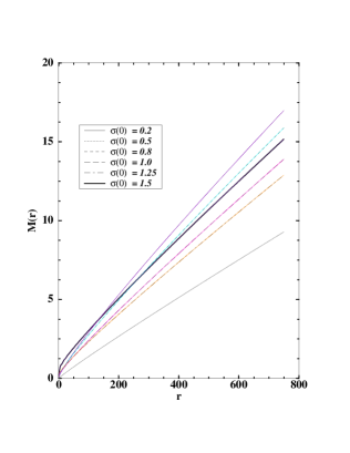
FIG. 1.: (a) Left: The mass profile of equilibrium configurations of massless scalar fields, are interestingly similar to the profiles of massive scalar fields and neutron stars. The mass for a given radius increases to a maximum with central density before it decreases with further increase in central density. However by calculating the particle number, we see no division into stable and unstable configurations at the peak. The particle number depends very sensitive on the initial value of the lapse function $N$, so that a clear cusp structure in the mass-particle-number diagram found for boson stars cannot be derived here (cf. [2, 8]). (b) Middle: The profiles are largely independent of radius although the mass itself increases with $r$. (c) Right: If one cuts the boson halos at the same energy density, then the mass profile reveals the same oscillating behavior as in case (a). The energy density $\rho$ is measured in $\omega^{2}/\kappa$.

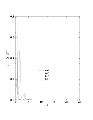
FIG. 2.: The inability of massless scalar field configurations to form compact self-gravitating objects as discussed by Christodoulou and others [12, 13] is verified numerically. An initial field configuration of the form $\sigma=0.001\cos(r)\exp(-r)$ is seen dispersing in the plot. The dispersion takes place very quickly.

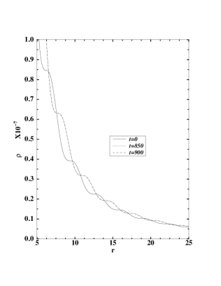
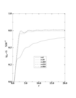
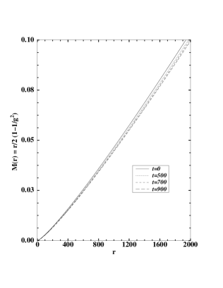
FIG. 3.: (a) Left: The formation of a self-gravitating massless scalar field object is shown here for an initial field configuration of the form $0.003\cos(r)(1-\exp(-1/r))$. The density in this case increases from its initial value as the configuration settles down. (b) Middle: The radial metric for this configuration is shown evolving to a stable final configuration. (c) Right: The mass is plotted as a function of radius at different times. As the configuration evolves it looses less and less mass as it settles down.

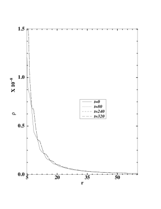
FIG. 4.: (a) Left: A Newtonian initial field configuration of the form $0.001\cos(r)/(r+1)$ can be regarded in some sense to be a perturbation of a Newtonian configuration which is proportional to $\sin(r)/r$. A plot of the density evolution is shown as it settles to a final stable state. Configurations of this form with non-Newtonian amplitudes do not settle down. Since the non-Newtonian configurations do not have this sinusoidal dependence this is not surprising. (b) Right: The radial metric evolution for the above configuration shows its settling in time.

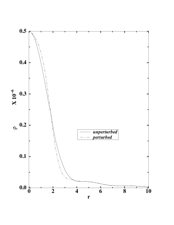
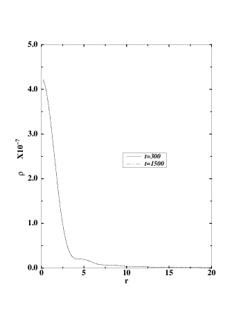
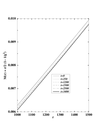
FIG. 5.: (a) Above left: An exact Newtonian configuration is perturbed and evolved. The initial unperturbed and perturbed densities are shown. A Gaussian amount of scalar field is removed from the equilibrium configuration and the constraint equations are reintegrated to give new metrics before beginning evolution. (b) Above right: The outgoing scalar radiation can be seen in a plot of the density at early times. (c) Bottom left: The density profile is shown after it starts to settle down. Between times of 300 and 1500 very little has changed in the density profile. (d) Bottom right: The mass is plotted as a function of radius for different times. In order to enhance the features only a small part of the radial region is shown. The amount of mass loss is clearly lessening in time.

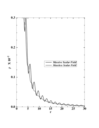
FIG. 6.: (a) Left: The density profiles of massive scalar field configurations with $\omega>m$ is compared to that of a massless field. The former has maxima and minima while the latter has saddle points. This structure may be related to stability issues. (b) Right: The mass and particle number are plotted against the central density for boson star oscillators. We find in all cases that the mass is always greater than the particle number explaining their instability against a collective dispersion.

TABLE I.: Mass values at different radii and different times for the evolution in Fig. 3. One recognizes that the change in the mass at fixed radius decreases, hence it proves the settling to a stable configuration.

Table 1.
	$t=0$	$t=500$	$t=700$	$t=900$
$r=800$	$0.03589375$	$0.0350625$	$0.034625$	$0.034234375$
$r=1200$	$0.0575$	$0.0563125$	$0.055625$	$0.0550625$
$r=1600$	$0.0801875$	$0.078625$	$0.0776875$	$0.0769375$

TABLE II.: Mass values at different radii and different times for the evolution in Fig. 5. One recognizes that the change in the mass at fixed radius decreases, hence it proves the settling to a stable configuration.

Table 2.
	$t=0$	$t=1500$	$t=2500$	$t=3400$
$r=500$	$0.002847$	$0.00278$	$0.0026875$	$0.00268375$
$r=1000$	$0.00628625$	$0.00619375$	$0.00608495$	$0.00608335$