Effects of anisotropy and spatial curvature on the pre-big bang scenario

Dominic Clancy^1a, James E. Lidsey^2b & Reza Tavakol^1c

¹Astronomy Unit, School of Mathematical Sciences,
Queen Mary & Westfield College, Mile End Road, LONDON, E1 4NS, U.K.

²Astronomy Centre and Centre for Theoretical Physics,
University of Sussex, BRIGHTON, BN1 9QH, U.K.

A class of exact, anisotropic cosmological solutions to the vacuum Brans–Dicke theory of gravity is considered within the context of the pre–big bang scenario. Included in this class are the Bianchi type III, V and ${\rm VI}_{h}$ models and the spatially isotropic, negatively curved Friedmann–Robertson–Walker universe. The effects of large anisotropy and spatial curvature are determined. In contrast to negatively curved Friedmann–Robertson–Walker model, there exist regions of the parameter space in which the combined effects of curvature and anisotropy prevent the occurrence of inflation. When inflation is possible, the necessary and sufficient conditions for successful pre–big bang inflation are more stringent than in the isotropic models. The initial state for these models is established and corresponds in general to a gravitational plane wave.

PACS NUMBERS: 04.20.Jb, 04.50.+h, 11.25.Mj, 98.80.Cq

^aElectronic address: dominic@maths.qmw.ac.uk

^bElectronic address: jel@astr.cpes.susx.ac.uk

^cElectronic address: reza@maths.qmw.ac.uk

1 Introduction

The inflationary paradigm of the very early universe resolves a number of problems with the hot big bang model [1]. In the standard, chaotic scenario, the inflationary (accelerated) expansion is driven by the potential energy of a self–interacting quantum scalar field [2]. Recently, an alternative inflationary cosmology – the pre–big bang scenario – has been developed within the context of string theory [3]. The fundamental postulate of pre–big bang cosmology is that the initial state of the universe should correspond to the string perturbative vacuum. Such a state is unstable to small fluctuations in the dilaton field, however, due to the non–minimal coupling of this field to the graviton. The kinetic energy of the dilaton then drives a superinflationary expansion, where the Hubble radius decreases with cosmic time, and the universe evolves from a region of weak coupling and low space–time curvature to one of strong coupling and high curvature. To lowest–order in the string effective action, the end state is a singularity both in the curvature and coupling, but it is anticipated that this will be avoided at the string scale when higher–order terms in the action become relevant [4]. An important feature of this scenario, therefore, is that the end of inflation is determined by quantum gravitational effects, in contrast to models driven by potential energy.

Given the potential importance of such a scenario, it is necessary to establish its generality with respect to anisotropy and spatial curvature, since small anisotropies and curvature are bound to be present in the real universe. A number of authors have recently addressed related questions. Veneziano and collaborators considered the general effects of small anisotropy and inhomogeneity by assuming the initial space and time derivatives of the fields were vanishingly small but of the same order [5, 6]. In this sense, the initial state of the universe is arbitrarily near to Minkowski space–time, but it is not necessarily homogeneous. It was found that sufficiently smooth regions inflate.

On the other hand, Turner and Weinberg investigated large spatial curvature in the isotropic Friedmann–Robertson–Walker (FRW) universes [7]. They concluded that curvature terms postpone the onset of inflation and can prevent sufficient inflation from occurring before higher–order terms become significant. This was interpreted as a restriction on the set of possible initial conditions. Kaloper, Linde and Bousso have also argued that initial conditions are severely constrained in the FRW models [8]. A Hamilton–Jacobi approach to inhomogeneous string cosmology has been developed [9] and higher–order corrections in spatially curved and anisotropic models have also been considered [10]. Finally, a number of exact anisotropic and inhomogeneous solutions have been found [11, 12, 13, 14].

The purpose of the present paper is to investigate the combined effects of spatial anisotropy and curvature in homogeneous, Brans–Dicke cosmologies. The Brans–Dicke theory includes the dilaton–graviton sector of the string effective action as a special case [15, 16]. We analyze the class of Bianchi type ${\rm VI}_{h}$ $(h<0)$ universes. These cosmologies are interesting for a number of reasons. They are amongst those Bianchi models with a positive measure in the homogeneous initial data and admit some of the most general, vacuum solutions [17]. They have a positive measure in the homogeneous initial data. Exact type ${\rm VI}_{h}$ solutions with a non–trivial dilaton field have been derived previously [18] and these solutions include the Bianchi types III and V and negatively curved, isotropic FRW models as special cases. Direct comparisons with the isotropic models can therefore be made by employing these solutions and, since they are exact, the effects of large deviations from the flat FRW model can also be determined. The initial state for a pre–big bang scenario can also be found analytically.

The paper is organised as follows. In Section 2 we present the cosmological solutions in the string frame, where fundamental strings trace geodesic surfaces with respect to the metric. We then determine whether large anisotropies and spatial curvature can prevent pre–big bang inflation. We derive quantitative bounds on the curvature and coupling for successful inflation in Section 3 and consider the early–time limits of the models in Section 4. We conclude with a discussion in Section 5.

Unless otherwise stated, units are chosen such that $\hbar=c=1$.

2 Pre–Big Bang Inflation in Bianchi Type ${\rm VI}_{h}$ Cosmologies

The Bianchi cosmologies are spatially homogeneous models with a line element given by $ds^{2}=-dt^{2}+h_{ij}(t)\omega^{i}\omega^{j}$ $(i,j=1,2,3)$, where $h_{ij}(t)$ is the metric on the surfaces of homogeneity and $\omega^{i}$ are one–forms [19]. A three–dimensional Lie group of isometries acts simply–transitively on the space–like, three–dimensional orbits and the structure constants, ${C^{a}}_{bc}$, of the Lie algebra of the group determine the isometry of the three–surfaces. In general, these may be expanded in terms of a diagonal, symmetric matrix, $m^{ab}$, such that ${C^{a}}_{bc}=m^{ad}\epsilon_{dbc}+{\delta^{a}}_{[b}a_{c]}$, where $a_{c}\equiv{C^{a}}_{ac}$ and indices are raised with $h^{ab}$ [20]. It then follows from the Jacobi identity, ${C^{a}}_{b[c}{C^{b}}_{de]}\equiv 0$, that $m^{ab}$ and $a_{b}$ must be orthogonal, $m^{ab}a_{b}=0$. A specific model belongs to the Bianchi class A or B if $a_{b}=0$ or $a_{b}\neq 0$, respectively [20]. Furthermore, each equivalence class of tensors ${C^{a}}_{bc}$ form a linear submanifold of the space of all 3–index tensors, where the dimension of each submanifold (with the upper bound of six) may be taken as a measure of that Bianchi class within the space of initial data. The class B Bianchi type ${\rm VI}_{h}$ models (with group parameter $h<0$) considered here are among the Bianchi models that possess the maximum dimension 6. When $h=-1$, this model corresponds to the Bianchi type III. The case $h=-1/9$ is exceptional because $a^{b}$ is not a shear eigenvector in this case [20]. The diagonal Bianchi type ${\rm VI}_{h}$ metric with ${m^{a}}_{a}=0$ is

$$ds^{2}=-dt^{2}+a_{1}^{2}(t)dx^{2}+a^{2}_{2}(t)e^{-2(1+k)x}dy^{2}+a_{3}^{2}(t)e^{2(k-1)x}dz^{2},$$ (2.1)

where $k\equiv(-h)^{-1/2}$.

The gravitational sector of the Brans–Dicke theory of gravity is given by [15]

$$S=\int d^{4}x\,\sqrt{-g}\,e^{-\phi}\left[R-\omega\left(\nabla\phi\right)^{2}\right]\,,$$ (2.2)

where $R$ is the Ricci curvature scalar of the spacetime with metric $g_{\mu\nu}$ and signature $(-,+,+,+)$, $g\equiv{\rm det}g_{\mu\nu}$ and $\phi$ is the dilaton field. The constant parameter $\omega$ determines the coupling between the dilaton and graviton and $\omega=-1$ corresponds to the string effective action [16]. The dilaton is assumed to be constant on the surfaces of homogeneity and the type ${\rm VI}_{h}$ cosmological field equations derived from Eq. (2.2) have the form

$$\partial_{t}{H}_{1}+3HH_{1}-2(1+k^{2})a_{1}^{-2}+\partial_{t}(\ln\Phi)\partial_{t}(\ln a_{1})=0$$

$$\partial_{t}{H}_{2}+3HH_{2}-2(1+k)a_{1}^{-2}+\partial_{t}(\ln\Phi)\partial_{t}(\ln a_{2})=0$$

$$\partial_{t}{H}_{3}+3HH_{3}-2(1-k)a_{1}^{-2}+\partial_{t}(\ln\Phi)\partial_{t}(\ln a_{3})=0$$

$$2H_{1}=(1+k)H_{2}+(1-k)H_{3}$$

$$H_{1}H_{2}+H_{1}H_{3}+H_{2}H_{3}-(3+k^{2})a_{1}^{-2}+3H\partial_{t}(\ln\Phi)-\frac{\omega}{2}\left[\partial_{t}(\ln\Phi)\right]^{2}=0$$

$$\partial_{t}\left(a^{3}\partial_{t}\Phi\right)=0,$$ (2.3)

where $\Phi\propto e^{-\phi}$ is the Brans-Dicke field, $a\equiv(a_{1}a_{2}a_{3})^{1/3}$ represents an averaged scale factor, $H_{i}\equiv\partial_{t}(\ln a_{i})$, $H\equiv\left(\sum_{i}H_{i}\right)/3$ and $\partial_{t}$ denotes differentiation with respect to cosmic time, $t$. The Brans–Dicke field determines the Planck length, $\Phi=l^{-2}_{\rm Pl}$, and, in string theory, is related to the string scale, $l_{\rm st}$, by $\Phi=l^{-2}_{\rm st}e^{-\phi}$.

The field equations (2.3) may be written as [18]

$$g^{\prime\prime}-4g = 0$$ (2.4)

$$(\ln y)^{\prime}+y(\ln g)^{\prime} = 2(1+k)$$ (2.5)

$$a_{2}a_{3}\Phi^{\prime} = -B,$$ (2.6)

where

$$g \equiv a_{2}a_{3}\Phi$$ (2.7)

$$y \equiv (\ln a_{2})^{\prime}$$ (2.8)

$$\eta \equiv \int^{t}\frac{dt_{1}}{a_{1}(t_{1})},$$ (2.9)

a prime denotes differentiation with respect to $\eta$ and $B$ is an arbitrary constant [18]. Eqs. (2.4)–(2.8) admit the class of solutions [18]

$$a_{1}^{2} = A_{1}^{2}\left[{\rm sinh}(-2\eta)\right]^{1+k^{2}}\left[{\rm tanh}(-\eta)\right]^{mk-p(1-k)}$$ (2.10)

$$a_{2}^{2} = A^{2}_{2}\left[{\rm sinh}(-2\eta)\right]^{1+k}\left[{\rm tanh}(-\eta)\right]^{m}$$ (2.11)

$$a_{3}^{2} = A_{3}^{2}\left[{\rm sinh}(-2\eta)\right]^{1-k}\left[{\rm tanh}(-\eta)\right]^{-(m+2p)}$$ (2.12)

$$\Phi = Q^{2}\left[{\rm tanh}(-\eta)\right]^{p},$$ (2.13)

where $A_{i}$ and $Q$ are arbitrary constants and the constants $\{m,p,k,\omega\}$ satisfy the constraint

$$3+k^{2}-m^{2}-2p\left[(\omega+2)p+m\right]=0.$$ (2.14)

A linear translation on the time parameter has been performed without loss of generality such that the singularity is located at $\eta=0$. We consider solutions defined over negative time within the context of the pre–big bang scenario.

Solution (2.10)–(2.13) includes the Bianchi type III, Bianchi type V and negatively curved FRW models as special cases, corresponding to $k=1$ $(h=-1)$, $k=0$ $(h=-\infty)$ and $(k=0,p=-m)$, respectively. It corresponds to the Ellis–MacCallum vacuum ${\rm VI}_{h}$ solution of Einstein gravity when the Brans–Dicke field is constant $(p=0)$ [20, 21]. In the limit $\eta\rightarrow 0^{-}$, it reduces to the Bianchi type I cosmology [22]:

$$a_{i}\propto(-\eta)^{p_{i}},\qquad\Phi\propto(-\eta)^{p},$$ (2.15)

where the constants $p_{i}$ are defined by

$$p_{1} \equiv \frac{1}{2}\left(1+k^{2}+mk-p(1-k)\right)$$

$$p_{2} \equiv \frac{1}{2}(1+k+m)$$

$$p_{3} \equiv \frac{1}{2}(1-k-2p-m)$$ (2.16)

and satisfy

$$\sum_{i=1}^{3}p_{i}=1+p_{1}-p.$$ (2.17)

The characteristic feature of pre–big bang cosmology is that the universe should exhibit superinflationary expansion simultaneously in all three directions as $t\rightarrow 0^{-}$ $(\eta\rightarrow 0^{-})$, i.e., $H_{i}>0$ and $\partial_{t}{H}_{i}>0$. We now consider the range of parameter values $\{k,m,p\}$ where this behaviour is possible. Due to continuity, it is sufficient to consider the necessary and sufficient conditions on the type I solution (2.15). These are that $p_{i}<0$ and $p_{1}>-1$ and this implies that

$$1<p(1-k)-k(k+m)<3$$

$$1+k+m<0$$

$$k+m+2p>1.$$ (2.18)

Thus, $p>0$ and the Brans–Dicke field must be a monotonically decreasing function of $\eta$.

The relevant regions in the $(m,p)$ plane for the type III and V models are illustrated in Figs. 1 and 2, respectively. For a given model, pre–big bang solutions are constrained to lie in the interior of the bold region defined by the constraints (2.18). In addition, physical solutions must satisfy Eq. (2.14). In the range $-3/2<\omega\leq 0$ (which includes the string case $\omega=-1$) and for all $k$, Eq. (2.14) represents an ellipse. The superinflationary solutions lie along the open arcs bounded by the points $AC$. In the type V model, the region of the ellipse consistent with the above constraints includes the point $B$ representing the negatively curved FRW solution $(p=-m=\sqrt{3})$. Although Eq. (2.14) implies that all type V solutions satisfy $|p|<\sqrt{3}$, only a very narrow region of the ellipse, $(1+\sqrt{5})/{2}<p<\sqrt{3}$, leads to pre–big bang inflation. Similar considerations give the allowed values of $m$ in this model to be $-\sqrt{5}<m<-1$.

Figure 1: Constraints on the parameters $m$ and $p$ permitting pre–big bang inflation in the Bianchi type III models. For $\omega=-1$, the bounds are $-2\sqrt{2}<m<-2$ and $\sqrt{2}<p<2$. The allowed region satisfying all constraints is given by the arc $AC$.

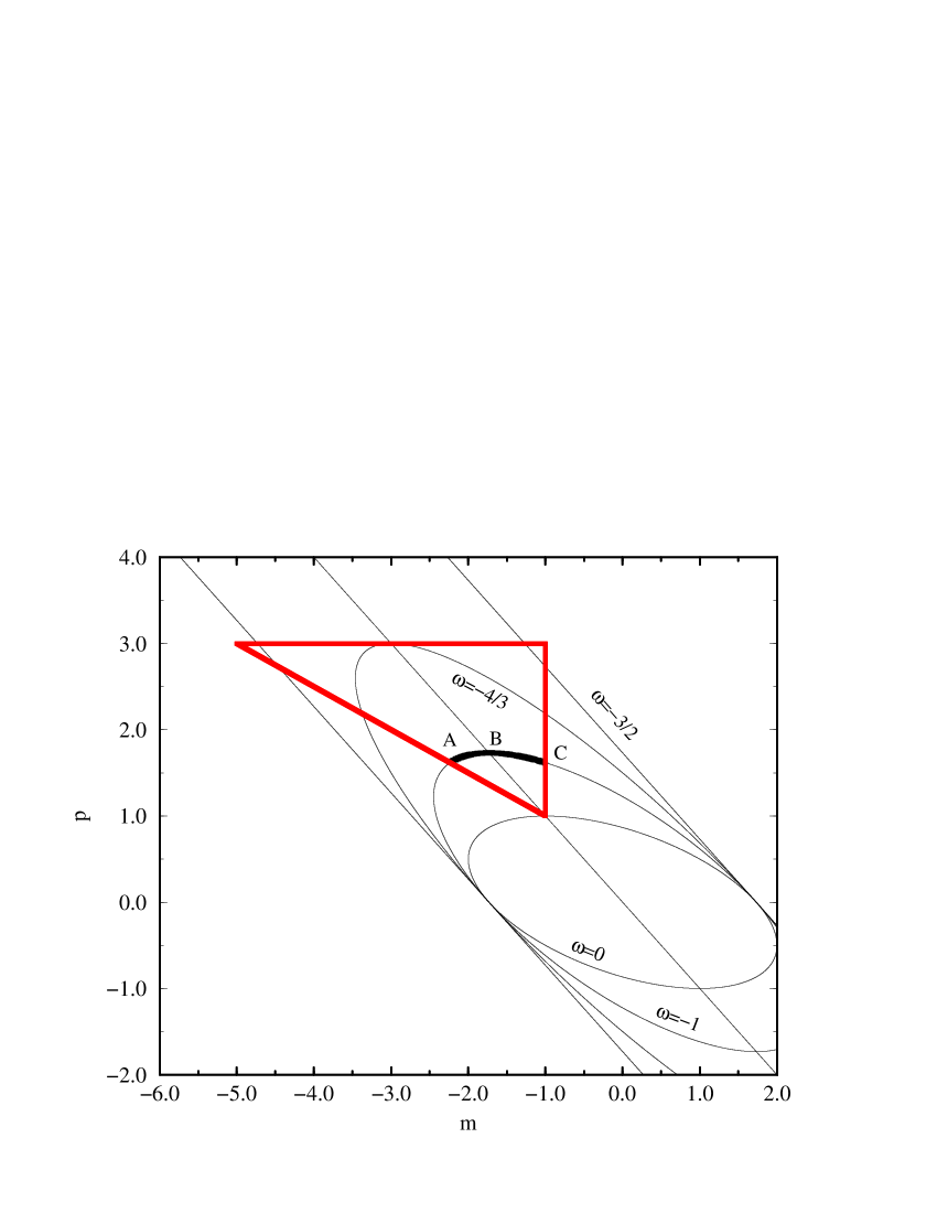
Figure 2: Constraints on the parameters $m$ and $p$ permitting pre–big bang inflation in the Bianchi type V models. The values of $m$ and $p$ must lie within the region bounded by $1<p<3$, $m<-1$ and $m+2p>1$. The arc $AC$ denotes the region satisfying all constraints in the string model and includes the point $B$ corresponding to the negatively curved FRW solution.

Thus, pre–big bang inflation is possible in these Bianchi models, but the combined roles of anisotropy and spatial curvature can prevent inflation from occurring. This is in contrast to the negatively curved FRW universe, where a superinflationary expansion towards a singular state is only delayed by the spatial curvature [7]. This is confirmed by our results shown in Fig. 2, since the point $B$ lies on the arc $AC$. When the FRW model is generalized to the anisotropic Bianchi type V universe, we find that only a relatively small region of the ellipse in Fig. 2 intersects the pre–big bang regime. Solutions exist in a region near to the FRW model $B$, where the anisotropy is small, but far from this point, superinflation does not proceed. In this sense, therefore, Fig. 2 provides in principle a quantitative measure of the likelihood of pre–big bang inflation for generic values of $(m,p)$ in the type V cosmology, given by the relative size of the arc AC to the allowed sections of the corresponding ellipse.

Finally, the ellipse (2.14) is also shown in Figs. 1 and 2 when $\omega=\{0,-4/3,-3/2\}$. The first two values represent the upper and lower bounds on $\omega$ consistent with pre–big bang inflation in the isotropic models [23]. In the anisotropic models considered here, the $\omega=0$ curve just intersects the bold–faced regions and this value again represents the upper limit on $\omega$ for the presence of superinflation. However, the lower bound is decreased to $\omega>-3/2$. (We do not consider $\omega<-3/2$ because this leads to a violation of the weak energy condition). It is interesting that the range of $\omega$ is broadened in these more general models and includes a simple class of higher–dimensional, Kaluza–Klein cosmologies [24].

In the following Section we derive bounds for successful pre–big bang inflation in the string–inspired model on the gravitational coupling and spatial curvature.

3 Conditions for successful inflation

In the Bianchi type ${\rm VI}_{h}$ models considered in the previous Section, the Brans–Dicke field begins to move move away from its asymptotic value when $\eta={\cal{O}}(-1)$. Its kinetic energy then increases significantly and this epoch denotes the onset of inflation. Since $p>0$, the effective gravitational coupling, $G\propto\Phi^{-1}$, diverges in the limit $\eta\rightarrow 0^{-}$. The question that now arises is whether sufficient inflation occurs before the regime of strong coupling and high space–time curvature is attained. Turner and Weinberg have derived bounds on the Brans–Dicke field for sufficient inflation in the open FRW model and have shown that the universe must be in the very small coupling and curvature regimes at the onset of the pre–big bang inflationary epoch [7]. Similar conclusions have been drawn in the inhomogeneous case [6]. We generalize these bounds to anisotropic, negatively curved universes.

The discussion following Fig. 2 implies that the initial anisotropy should not be too pronounced and, consequently, we assume that $a_{1}={\cal{O}}(a_{2})={\cal{O}}(a_{3})$ when $\eta={\cal{O}}(-1)$. We further assume that spatial curvature rapidly becomes negligible once inflation begins and that the Bianchi type I solution (2.15) applies for $\eta>-1$. The amount of inflation that occurs in each direction is given by the ratio

$$Z_{i}\equiv\frac{H_{if}a_{if}}{H_{ib}a_{ib}},$$ (3.1)

where subscripts ‘$b$’ and ‘$f$’ denote values at the onset and end of inflation, respectively. Substitution of Eq. (2.15) into Eq. (3.1) implies that

$$Z_{i}\approx\left(\frac{\eta_{b}}{\eta_{f}}\right)^{1+p_{1}-p_{i}}\approx\left(\frac{\Phi_{b}}{\Phi_{f}}\right)^{(1+p_{1}-p_{i})/p}\approx\left(\frac{H_{if}}{H_{ib}}\right)^{(1+p_{1}-p_{i})/(1+p_{1})},$$ (3.2)

where $\Phi_{b}\approx Q^{2}$. In general, the inflationary solution derived from the tree–level string effective action breaks down at $t\approx t_{f}$ when either the coupling exceeds the critical value $\Phi^{-1}(t_{f})\approx l_{\rm st}^{2}$ or the curvature becomes comparable to the string scale, $H^{2}_{i}(t_{f})\approx l_{\rm st}^{-2}$. Substituting these conditions into Eq. (3.2) then implies that

$$Z_{i}<{\rm Min}\left\{\left(Q^{2}l_{\rm st}^{2}\right)^{(1+p_{1}-p_{i})/p},\left(H_{ib}l_{\rm st}\right)^{(p_{i}-1-p_{1})/(1+p_{1})}\right\}.$$ (3.3)

Since $\eta_{b}={\cal{O}}(-1)$, it follows that $\Phi(-\eta_{b})\approx-\Phi^{\prime}(-\eta_{b})$. Moreover, approximating the solution to that of the type I cosmology implies that $H_{i}\approx-p_{i}/[A_{1}(-\eta)^{1+p_{1}}]$, and, therefore, that $H_{ib}\approx 1/A_{1}$. The definition (2.6) then implies that $H_{ib}\approx(Q^{2}/B)^{1/2}$. Substituting these relationships into Eq. (3.3) and combining the two inequalities leads to an upper limit on the amount of pre–big bang inflation in each of the three spatial directions:

$$Z_{i}\leq B^{r_{i}}\approx\left(-\dot{\Phi}_{b}a^{3}_{b}\right)^{r_{i}},\qquad r_{i}\equiv\frac{1+p_{1}-p_{i}}{2(1+p_{1})+p},$$ (3.4)

where a dot denotes differentiation with respect to cosmic time, $t$.

This expression generalizes the result of Turner and Weinberg [7] to the class of negatively curved, anisotropic cosmological models that exhibit similar qualitative behaviour to that of the type ${\rm VI}_{h}$ model. The effect of the anisotropy on the maximum amount of inflation is parametrized completely in terms of the exponents $r_{i}$. The constraints (2.18) ensure that these quantities are positive definite and they take the values $r_{i}=1/3$ in the isotropic FRW limit. Successful inflation requires that all directions expand by factors of at least $Z_{i}\geq e^{60}$ [1] and this implies that $B\geq{\rm exp}(60/r_{i})$. Consequently, the spatial direction with the smallest exponent determines the strongest limit on the value of $B=-\dot{\Phi}a^{3}$. The constraint is weakest when $r_{i}$ are simultaneously maximized. Since $\sum_{i}r_{i}=1$ and $r_{i}>0$, their maximal values correspond to the isotropic limit, $r_{i}=1/3$. We conclude, therefore, that a necessary, but not sufficient, condition for successful inflation is $-\dot{\Phi}a^{3}\geq e^{180}$. This becomes a sufficient condition only in the isotropic limit. This implies that the constraints in anisotropic models are stronger than in the isotropic case.

The inflation factors in the type V model are bounded such that

$$Z_{1}\leq B^{1/3},\qquad Z_{2}\leq B^{(2-p-m)/6},\qquad Z_{3}\leq B^{(2+p+m)/6}.$$ (3.5)

Either one of the exponents $r_{2}$ or $r_{3}$ is minimized when $|p+m|$ is maximized and this occurs when $|p+m|\rightarrow(\sqrt{5}-1)/2$. Substituting this limiting value into the constraint (3.5) implies that $B\geq e^{260}$ is a sufficient condition for successful type V pre–big bang inflation. For the Bianchi type III model, the constraints on the inflation factors are

$$Z_{1}=Z_{2}\leq B^{1/(4+m+p)},\qquad Z_{3}\leq B^{(2+m+p)/(4+m+p)}.$$ (3.6)

In this model, $p+m<0$, and the exponents $r_{1}=r_{2}$ are maximized (minimized) when $|p+m|$ is maximized (minimized). It follows from Eqs. (2.14) and (2.18) that the minimum values the exponents may take are $r_{1}=r_{2}=0.25$ and $r_{3}=0.23$. Thus, the corresponding sufficient bound for successful inflation in this model is $B\geq e^{240}$.

Finally, instead of imposing initial conditions in the limit $t\rightarrow-\infty$, one may consider a scenario where quantum stringy effects result in the spontaneous creation of a sufficiently homogeneous universe at a time $\eta=\eta_{0}$ [7]. In this case, inflation will not begin immediately if $|\eta_{0}|>|\eta_{b}|$ and Eq. (3.4) then determines the total amount of inflation that is possible.

If, on the other hand, $|\eta_{0}|<|\eta_{b}|$, inflation begins immediately, but Eq. (3.4) overestimates the amount of inflation because the expansion during the epoch $\eta_{b}<\eta<\eta_{0}$ does not occur. Thus, the actual amount of inflation is given by

$$Z_{i,{\rm actual}}=\frac{H_{ib}a_{ib}}{H_{i0}a_{i0}}Z_{i}\approx\left(\frac{\eta_{b}}{\eta_{0}}\right)^{p_{i}-1-p_{1}}Z_{i}.$$ (3.7)

By employing the relations $a^{2}\Phi\propto(-\eta)^{(2+2p_{1}+p)/3}$ and $B\approx a^{2}_{b}\Phi_{b}$, together with Eqs. (2.6) and (3.4), we find that

$$Z_{i,{\rm actual}}\leq\left(\frac{\Phi_{0}^{3}}{\dot{\Phi}^{2}_{0}}\right)^{r_{i}}.$$ (3.8)

Thus, the coupling must be sufficiently small at $\eta=\eta_{0}$ if enough inflation is to occur.

4 Past asymptotic state of the universe

It is important to consider the initial state of the universe as $t\rightarrow-\infty$. Recently, Buonanno et al. have conjectured that with sufficiently isotropic initial data, the Milne universe represents an attractor in the far past for negatively curved cosmologies [6]. The Milne universe represents the wedge of Minkowski space–time corresponding to the future (past) light–cone, $|t|>|{\rm{\bf x}}|$, of the origin. In this sense, it corresponds to the string perturbative vacuum and its spatial three–sections, $t={\rm constant}$, are constant curvature hyperbolic surfaces [25]. The exact, negatively curved FRW solutions with radiation and non–trivial axion, dilaton and moduli fields approach the Milne solution in the infinite past [7, 11].

In this Section we determine the initial state of the class of type ${\rm VI}_{h}$ cosmologies (2.10)–(2.13) within the context of the pre–big bang scenario without restricting the level of anisotropy. As $\eta\rightarrow-\infty$, the dilaton tends to a constant value and the metric (2.1) reduces to the vacuum solution of Lifshitz and Khalatnikov [26]:

$$ds^{2}=-dt^{2}+(1+k^{2})^{2}(-t)^{2}dx^{2}+e^{-2(1+k)x}(-t)^{2(1+k)/(1+k^{2})}dy^{2}$$

$$+e^{2(k-1)x}(-t)^{2(1-k)/(1+k^{2})}dz^{2},$$ (4.1)

where the variables $\{y,z\}$ have been rescaled without loss of generality. Defining the coordinate pair

$$u\equiv(-t)e^{-(1+k^{2})x},\qquad v\equiv(-t)e^{(1+k^{2})x}$$ (4.2)

transforms the metric (4) to the null form

$$ds^{2}=-dudv+u^{2(1+k)/(1+k^{2})}dy^{2}+u^{2(1-k)/(1+k^{2})}dz^{2}$$ (4.3)

and a further change of variables:

$$v\equiv\bar{v}-\frac{1}{u(1+k^{2})}\left(\bar{y}^{2}+\bar{z}^{2}+2k\bar{y}\bar{z}\right)$$

$$y\equiv\frac{1}{\sqrt{2}}u^{-(1+k)/(1+k^{2})}(\bar{y}+\bar{z})$$

$$z\equiv\frac{1}{\sqrt{2}}u^{-(1-k)/(1+k^{2})}(\bar{y}-\bar{z})$$ (4.4)

implies that

$$ds^{2}=-dud\bar{v}+F(u,\bar{y},\bar{z})du^{2}+d\bar{y}^{2}+d\bar{z}^{2},$$ (4.5)

where

$$F(u,\bar{y},\bar{z})\equiv H(u)\bar{y}\bar{z},\qquad H(u)\equiv\frac{2k(1-k^{2})}{(1+k^{2})^{2}}u^{-2}.$$ (4.6)

In general, Eq. (4.5) is the metric for a gravitational plane wave with an amplitude uniquely determined by the function $H(u)$ [17, 26, 27]. (For a review of the properties of plane wave metrics see, e.g., Ref. [28]). These metrics are Ricci–flat and exhibit a covariantly constant null Killing vector field, $l_{\mu}\equiv\partial_{\mu}u$, where $l^{\mu}\partial_{\mu}\bar{v}=1$, and the Riemann curvature is given by $R_{\mu\nu\rho\sigma}=2l_{[\mu}\partial_{\nu]}\partial_{[\rho}Fl_{\sigma]}$. It follows that the only non–zero component is $R_{u\bar{y}u\bar{z}}=-\frac{1}{2}H(u)$ and for $k\neq\{0,1\}$, this tends to zero as $|u|\rightarrow+\infty$.

It follows that in the limit of $\eta\rightarrow-\infty$, where the metric (2.1) reduces to (4), the Riemann curvature is identically zero for the Bianchi types III and V. Thus, the initial state of these models is isomorphic to the string perturbative vacuum and substituting the new variables

$$-t \equiv \left[T^{2}-X^{2}-Y^{2}-(1-k)Z^{2}\right]^{1/2}$$ (4.7)

$$x \equiv \frac{1}{2(1+k)}\ln\left[\frac{T^{2}-X^{2}-Y^{2}-(1-k)Z^{2}}{(T-X)^{2}}\right]$$ (4.8)

$$y \equiv \frac{Y}{T-X}$$ (4.9)

$$z \equiv \frac{Z}{(T-X)^{1-k}}$$ (4.10)

into Eq. (4) transforms the metric into the standard Minkowski form, $d\eta^{2}=-dT^{2}+dX_{i}dX^{i}$, when $k=\{0,1\}$.

It is important to note that the entire Minkowski space–time is not covered by the set of coordinates (4.7)–(4.10). The type V model is isomorphic to the wedge representing the $(3+1)$–dimensional Milne universe. In the type III model, there is no restriction from the $Z$ coordinate on the timelike variable, $T$, and this background is formally equivalent to the product of the $(2+1)$–dimensional Milne model with a line. The asymptotic behaviour of these exact type III and V solutions are therefore consistent with the conjecture of Buonanno et al. [6].

5 Discussion and Conclusion

In this paper we have considered the pre–big bang scenario within the context of the spatially homogeneous, diagonal Bianchi type ${\rm VI}_{h}$ universes, including the types III, V and negatively curved FRW models as particular cases. We find that the combined effects of anisotropy and spatial curvature can prevent pre–big bang inflation, in contrast to the negatively curved FRW cosmology. In the region of parameter space where inflation does occur, the gravitational coupling and spatial curvature must satisfy appropriate bounds for successful inflation. In general, these bounds are stronger in the anisotropic models than the FRW models. In particular, the constraint $\ln(-\dot{\Phi}a^{3})>180$ is a sufficient condition for successful inflation in the FRW universe, but this is strengthened to $\ln(-\dot{\Phi}a^{3})>260$ in the type V model.

The past asymptotic state of the models was established. In general, the asymptotic behaviour of the scale factors (2.10)–(2.12) would seem to indicate that the universe must have been highly anisotropic and infinitely large in the far past and it could be argued that such a state is unnatural [7, 8]. However, the type III and V models are isomorphic to the wedge of Minkowski space–time (string perturbative vacuum) corresponding to the Milne universe with an asymptotically constant dilaton field. This is in agreement with the postulates of the pre–big bang cosmology.

On the other hand, we have found that the asymptotic limit of the generic diagonal type ${\rm VI}_{h}$ cosmology with a dilaton corresponds to a homogeneous gravitational plane wave. This supports the conjecture that Bianchi type IV, ${\rm VI}_{h}$ and ${\rm VII}_{h}$ models containing a perfect fluid with pressure $p$ and energy density $\rho$ related by $p=(\gamma-1)\rho$ $(2/3<\gamma\leq 2)$ are asymptotic to a plane wave model or the Collins ${\rm VI}_{h}$ model [29, 30].

There are a number of reasons why plane wave backgrounds represent a generic initial state for the universe in the pre–big bang scenario. Firstly, in the space of initial data, the most general vacuum Bianchi type B models are the types ${\rm VI}_{h}$ and ${\rm VII}_{h}$. All but a set of measure zero of the known (asymptotically self–similar) solutions belonging to these types correspond to gravitational plane waves [17, 30, 31, 32]. These solutions have been classified in a unified manner by Siklos [17] and recently surveyed in Ref. [33].

Secondly, gravitational plane waves are manifestly Ricci–flat and exhibit the important property that their curvature invariants vanish identically. Consequently, they are exact solutions to the classical string equations of motion to all orders in the inverse string tension [34]. Moreover, both the ${\rm VI}_{h}$ and ${\rm VII}_{h}$ vacuum solutions exhibit unbroken space–time supersymmetries with constant Killing spinors [34, 35]. This is important because supersymmetric solutions have a nonrenormalization property and therefore play a central role in quantum theories of gravity [36]. It has been suggested that supersymmetric plane waves may provide a suitable basis for an expansion of the path integral in quantum string gravity and such an approach may yield further insight into the high curvature, strong–coupling regime of the pre–big bang scenario.

Finally, higher dimensions are important in any realistic string cosmology. Recent advances in string theory indicate that the five separate theories have a common origin in an eleven–dimensional ‘M–theory’, where the radius of the eleventh dimension is related to the dilaton, $R_{11}\approx l_{\rm st}e^{\phi/3}$ [37, 38]. Within the context of M–theory, the thickness of the eleventh dimension should be vanishingly small if the initial state of the universe is the ten–dimensional string perturbative vacuum with vanishing coupling $(\phi\rightarrow-\infty)$. Since the low–energy effective action of M–theory is eleven–dimensional supergravity with a vacuum limit given by Einstein gravity [39], a possible initial state that avoids such a difficulty is an eleven–dimensional gravitational plane wave manifold that is homeomorphic to ${\cal R}^{11}$.

It would be interesting to consider the implications of such an initial state further. In particular, the embedding of four–dimensional cosmological solutions in such an eleven-dimensional background could be established by employing the known theorems of differential geometry. For example, there exists a theorem that states that any $n$–dimensional Riemannian manifold may be locally and isometrically embedded in a Ricci–flat, Riemannian manifold of arbitrary dimension, $N\geq n+1$ [40]. A number of plane wave solutions were recently embedded in five–dimensional spaces by employing such a theorem [41].

The bounds on the coupling and curvature derived in this paper correspond to the string model, $\omega=-1$, and it would be interesting to generalize the results to other values of $\omega$. It would also be of interest to extend the analysis to include other fields that arise in the low–energy string effective action. Homogeneous solutions with a non–trivial Neveu–Schwarz/Neveu–Schwarz (NS–NS) form field have been found for a wide variety of Bianchi and Kantowski–Sachs models [11, 12, 13]. These solutions may serve as a basis for investigating whether the bounds for successful inflation in highly anisotropic models are altered when such a form field is present. Their asymptotic limits could also be investigated to establish whether class B cosmologies containing both a dilaton and NS–NS form field asymptotically approach a plane wave model.

In conclusion, therefore, spatial curvature and anisotropy lead to a number of important physical effects in the pre–big bang scenario.

Acknowledgments

DC and JEL are supported by the Particle Physics and Astronomy Research Council (PPARC), UK. JEL thanks the Astronomy Unit, Queen Mary and Westfield, and the Theory Division, CERN, for hospitality. We thank J. D. Barrow, N. P. Dabrowski, J. Maharana, S. T. C. Siklos, M. S. Turner and G. Veneziano for helpful discussions and communications.

References

References

- [1] A. A. Starobinsky, Phys. Lett. B 91, 99 (1980); A. H. Guth, Phys. Rev. D 23, 347 (1981); K. Sato, Mon. Not. R. Astron. Soc. 195, 467 (1981); A. D. Linde, Phys. Lett. B 108, 389 (1982); A. Albrecht and P. J. Steinhardt, Phys. Rev. Lett. 48, 1220 (1982); S. W. Hawking and I. G. Moss, Phys. Lett. B 110, 35 (1982).
- [2] A. D. Linde, Phys. Lett. B 129, 177 (1983); A. D. Linde, Particle Physics and Inflationary Cosmology (Harwood Academic, Chur, Switzerland, 1990).
- [3] G. Veneziano, Phys. Lett. B 265, 287 (1991); M. Gasperini and G. Veneziano, Astropart. Phys. 1, 317 (1993); M. Gasperini and G. Veneziano, Mod. Phys. Lett. A 8, 3701 (1993); M. Gasperini and G. Veneziano, Phys. Rev. D 50, 2519 (1994).
- [4] R. Brustein and G. Veneziano, Phys. Lett. B 329, 429 (1994); N. Kaloper, R. Madden, and K. A. Olive, Nucl. Phys. B 452, 677 (1995); N. Kaloper, R. Madden, and K. A. Olive, Phys. Lett. B 371, 34 (1996); R. Easther, K. Maeda, and D. Wands, Phys. Rev. D 53, 4247 (1996).
- [5] G. Veneziano, Phys. Lett. B 406, 297 (1997).
- [6] A. Buonanno, K. A. Meissner, C. Ungarelli, and G. Veneziano, “Classical inhomogeneities in string cosmology”, hep-th/9706221.
- [7] M. S. Turner and E. J. Weinberg, Phys. Rev. D 56, 4604 (1997).
- [8] N. Kaloper, A. Linde, and R. Bousso, “Pre–big bang requires the universe to be exponentially large from the very beginning”, hep-th/9801073.
- [9] K. Saygili, “Hamilton–Jacobi approach to pre–big bang cosmology at long–wavelengths”, hep-th/9710070.
- [10] M. Maggiore and R. Sturani, “The fine tuning problem in pre–big bang inflation”, gr-qc/9706053, In Press, Phys. Lett. B (1998).
- [11] E. J. Copeland, A. Lahiri, and D. Wands, Phys. Rev. D 50, 4868 (1994); E. J. Copeland, A. Lahiri, and D. Wands, Phys. Rev. D 51, 223 (1995).
- [12] N. A. Batakis and A. A. Kehagias, Nucl. Phys. B 449, 248 (1995); N. A. Batakis, Phys. Lett. B 353, 39 (1995); N. A. Batakis, Phys. Lett. B 353, 450 (1995); N. A. Batakis and A. A. Kehagias, Phys. Lett. B 356, 223 (1995).
- [13] J. D. Barrow and K. Kunze, Phys. Rev. D 55, 623 (1997); J. D. Barrow and M. P. Dabrowski, Phys. Rev. D 55, 630 (1997).
- [14] J. D. Barrow and K. Kunze, Phys. Rev. D 56, 741 (1997); A. Feinstein, R. Lazkoz, and M. A. Vazquez-Mozo, Phys. Rev. D 56, 5166 (1997); M. Giovannini, “Regular cosmological examples of tree–level dilaton–driven models”, hep-th/9712122.
- [15] C. Brans and R. H. Dicke, Phys. Rev. 124, 925 (1961).
- [16] M. B. Green, J. H. Schwarz, and E. Witten, Superstring Theory: Vol. 1 (Cambridge University Press, Cambridge, 1987).
- [17] S. T. C. Siklos, Commun. Math. Phys. 58, 255 (1978); S. T. C. Siklos, J. Phys. A 14, 395 (1981); S. T. C. Siklos, in Relativistic Astrophysics and Cosmology, eds. X. Fustero and E. Verdaguer (World Scientific, Singapore, 1984).
- [18] D. Lorenz–Petzold, Astrophys. Space Sci. 98, 101 (1984).
- [19] M. P. Ryan and L. C. Shepley, Homogeneous Relativistic Cosmologies (Princeton University Press, Princeton, 1975).
- [20] G. F. R. Ellis and M. A. H. MacCallum, Commun. Math. Phys. 12, 108 (1969).
- [21] M. A. H. MacCallum, Commun. Math. Phys. 20, 57 (1971).
- [22] M. Mueller, Nucl. Phys. B 337, 37 (1990).
- [23] J. E. Lidsey, Phys. Rev. D 55, 3303 (1997).
- [24] T. Appelquist, A. Chodos, and P. G. O. Freund, Modern Kaluza–Klein Theories (Addison–Wesley, New York, 1987).
- [25] N. D. Birrell and P. C. W. Davies Quantum Fields in Curved Space (Cambridge University Press, Cambridge, 1982).
- [26] E. M. Lifshitz and I. M. Khalatnikov, Adv. Phys. 12, 185 (1963); J. Wainwright, Phys. Lett. A 99, 301 (1983).
- [27] H. Brinkmann, Proc. Natl. Acad. Sci. USA 9, 1 (1923); H. Brinkmann, Math. Ann. 94, 119 (1925).
- [28] D. Kramer, H. Stephani, E. Herlt, and M. A. H. MacCallum, Exact Solutions of Einstein’s Field Equations (Cambridge University Press, Cambridge, 1980).
- [29] C. B. Collins, Commun. Math. Phys. 23, 137 (1971).
- [30] C. G. Hewitt and J. Wainwright, Class. Quantum Grav. 10, 99 (1993); C. G. Hewitt and J. Wainwright, in Dynamical Systems in Cosmology, eds. J. Wainwright and G. F. R. Ellis (Cambridge University Press, Cambridge, 1996).
- [31] V. Lukash, Sov. Phys. JETP 40, 792 (1975).
- [32] J. D. Barrow and D. H. Sonoda, Phys. Rep. 139, 1 (1986).
- [33] C. G. Hewitt, S. T. C. Siklos, C. Uggla, and J. Wainwright, in Dynamical Systems in Cosmology, eds. J. Wainwright and G. F. R. Ellis (Cambridge University Press, Cambridge, 1996).
- [34] R. Güven, Phys. Lett. B 191, 275 (1987).
- [35] E. A. Bergshoeff, R. Kallosh, and T. Ortin, Phys. Rev. D 47, 5444 (1993).
- [36] A. Dabholkar, G. Gibbons, J. A. Harvey, and F. Ruiz, Nucl. Phys. B 340, 33 (1990); R. E. Kallosh, A. D. Linde, T. M. Ortin, A. W. Peet, and A. Van Proeyen, Phys. Rev. D 46, 5278 (1992).
- [37] A. Font, L. Ibanez, D. Luest, and F. Quevedo, Phys. Lett. B 249, 35 (1990); A. Sen, Int. J. Mod. Phys. A 9, 3707 (1994); A. Giveon, M. Porrati, and E. Rabinovici, Phys. Rep. 244, 77 (1994); J. Polchinski and E. Witten, Nucl. Phys. B 460, 525 (1996); J. Polchinski, Rev. Mod. Phys. 68 1245 (1996).
- [38] E. Witten, Nucl. Phys. B 443, 85 (1995); J. H. Schwarz, Phys. Lett. B 367, 97 (1996); M. J. Duff, Int. J. Mod. Phys. A 11, 5623 (1996).
- [39] E. Cremmer and B. Julia, Nucl. Phys. B 159, 141 (1978).
- [40] J. E. Campbell, A Course of Differential Geometry (Clarendon Press, Oxford, 1926); C. Romero, R. Tavakol, and R. Zalaletdinov, Gen. Rel. Grav. 28, 365 (1996); J. E. Lidsey, R. Tavakol, and C. Romero, Mod. Phys. Lett. A 12, 2319 (1997).
- [41] J. E. Lidsey, C. Romero, R. Tavakol, and S. Rippl, Class. Quantum Grav. 14 865 (1997); J. E. Lidsey, In press, Phys. Lett. B (1998).