Einstein-Yang-Mills black hole solutions
in three dimensions.

Introduction.

Solutions of Einstein-Yang-Mills (EYM) equations have already been the motivation for several studies [1]. For most of them the ansatz used is a sophisticated version of the Reissner-Nordstr m solution. This solution teaches a lot about the properties of EYM black holes, but it requires a numerical evaluation in the final stage. Here, a method is proposed to build analytically a family of Euclidean solutions to these equations. In this report, the method is restricted to three dimensions and SU(2) is chosen as the Yang-Mills (YM) group.

The study of 3 dimensional gravity is important because it provides a compromise between the triviality of 2-d gravity and the intricacy of the 4-d one. Classically, the Riemann tensor is entirely determined by the Ricci tensor and by the scalar curvature, thus the solutions of the Einstein equations can be studied almost systematically [2]. From the quantum point of view, the formalism proposed by Achùcarro, Townsend, Witten [3, 4] shows that 3-d quantum gravity is, in principle, integrable [4] albeit not trivial. It can serve as a good model for exploring the complexity of quantum gravity [5] or at least of quantum field theory in curved space-time.

The study of quantum properties by a functional integral means that one has to look for Euclidean solutions that will provide a starting point for a saddle point approximation. This method has shown its efficiency in the development of black hole thermodynamical properties and in quantum cosmology [6]. An important step is to introduce non-trivial matter fields such as the YM field in this procedure.

In the present work, the key to finding Euclidean solutions for the EYM equations is based on describing the 3-d YM theory in terms of gauge invariant variables [7]. In this procedure, YM theory takes the form of a gravity. Thus, the EYM equations reduce to those of two coupled gravities. The similarity between the two sets of equations leads to a very simple ansatz which reduces the two coupled equations to one simple Einstein equation.

We apply our ansatz to the Euclidean continuation of BTZ black hole which is a particularly interesting three dimensional solution [8] of the Einstein equations. The mass and the energy of the solution are calculated with the help of the quasi-local formalism developed in [9] and [10].

Reformulation of the 3d SU(2) Yang-Mills theory as a Euclidean
gravity.

The reformulation of a YM theory as a strong gravity is based on the idea that there can exist a combination of YM fields which can be defined as a new metric on space-time. This is a very difficult task in four dimensions but some elegant ways exist in three dimensions such as, for example, the Lunev reformulation [7]. This reformulation is reviewed in the following, with a few modifications that will allow it to be adapted to our problem. Consider the SU(2) YM theory written in first order formalism, on a 3-dimensional Euclidean manifold $\mathcal{M}$ with a metric $g_{\mu\nu}$:

$$S_{\mathrm{Y}M}=\frac{1}{16\pi\alpha_{{}_{\rm{s}}}}\int_{\mathcal{M}}d^{3}x\sqrt{g}\Big{(}2F_{a}^{\ \mu\nu}(\partial_{\mu}A^{a}_{\nu}-\partial_{\nu}A^{a}_{\mu}-\epsilon^{abc}A_{b\mu}A_{c\nu})-F_{a}^{\ \mu\nu}F^{a}_{\ \mu\nu}\Big{)}$$ (1)

Where $\alpha_{{}_{\rm{s}}}$ is the square of the YM coupling constant.

Instead of $(F^{a}_{\ \mu\nu},A^{a}_{\mu})$ one can choose $(E^{a}_{\mu},A^{a}_{\mu})$ as the fundamental variables where:

$$E^{a}_{\rho}=-\frac{1}{\alpha_{{}_{\rm{s}}}^{2}}{\sqrt{g}\over 2}\epsilon_{\rho\mu\nu}\,F^{a\mu\nu}$$ (2)

The new variable $E^{a}_{\rho}$ is simply the dual variable of $F^{a}_{\ \mu\nu}$. The term $(\alpha_{{}_{\rm{s}}})^{-2}$ which has, in 3d, the dimension of L², is added to the definition in order to obtain dimensionless quantities. This is necessary because we want to interpret

$$G_{\mu\nu}=E^{a}_{\mu}\,\delta_{ab}\,E^{b}_{\nu}$$ (3)

as a new metric field on space. The minus sign in Eq. (2) is used in order to ensure that the strong gravitational constant will always have the same sign as the universal gravitational constant. In three dimensions there is, strictly speaking, no gravitational interaction and so a negative gravitational constant does no harm. If $\det(E)~{}>~{}0$ on $\mathcal{M}$ except eventually on a null measure set, then by substituting Eq. (2) in Eq. (1), $S_{\mathrm{Y}M}$ can be rewritten as [7]

$$S_{\mathrm{Y}M}=-\frac{\alpha_{{}_{\rm{s}}}}{4\pi}\int_{\mathcal{M}}d^{3}x\Big{\{}\sqrt{G}R(\Gamma)+\frac{\alpha_{{}_{\rm{s}}}^{2}}{2}\sqrt{g}g^{\mu\nu}G_{\mu\nu}\Big{\}}$$ (4)

where $G_{\mu\nu}$ is the strong metric defined in Eq. (3), $\sqrt{G}=\sqrt{\det(G_{\mu\nu})}$, $\Gamma$ is the strong gravitational connection defined by:

$${\mathcal{D}}_{\mu}\,E^{a}_{\nu}\equiv\partial_{\mu}\,E^{a}_{\nu}-\epsilon^{abc}A_{b\mu}E_{c\nu}-\Gamma^{\rho}_{\nu\mu}E^{a}_{\rho}\equiv 0$$ (5)

and $R(\Gamma)$ is the scalar curvature of $\Gamma$. One can see that the vacuum YM equations can be written as:

$$\epsilon^{\lambda\mu\nu}D_{\mu}\,E^{a}_{\nu}=0$$

In conjunction with Eq. (5) this implies that if there are no YM sources, then $\Gamma$ is torsion free i.e.

$$T^{\mu}_{\,\nu\rho}(\Gamma)=0$$ (6)

The first part of Eq. (4) is nothing but a pure Euclidean Einstein gravity action in its first order (or Palatini) formulation. The Euclidean character of this gravity is imposed by the signature of the su(2) Killing metric: $\frac{1}{2}\delta_{ab}$. One can remark that the Newton constant of this gravity is $G_{\mathcal{S}}=(4\alpha_{{}_{\rm{s}}})^{-1}$. The second part introduces a coupling between the new metric and the universal one. This term is not surprising because the YM action depends on the metric $g_{\mu\nu}$ which must appear somewhere in the reformulation.

The reformulation can have several applications such as, for example, the study of the new degree of freedom $G_{\mu\nu}$ and the study of confinement [11]. We will concentrate on the search of solutions to the EYM equations where it appears to be very powerful.

Reformulated Einstein-Yang-Mills equations.

We are now interested in the complete EYM action:

$$S=\int_{\mathcal{M}}d^{3}x\sqrt{g}\Big{(}\frac{1}{16\pi\alpha_{{}_{\rm{s}}}}F^{a}_{\ \mu\nu}F_{a}^{\ \mu\nu}-\frac{1}{16\pi G_{\mathcal{N}}}(r(\gamma)+2\Lambda)\Big{)}+S_{B}$$ (7)

where $G_{\mathcal{N}}$ is the Newton constant, $r$ the scalar curvature of the connection $\gamma$, $\Lambda$ the cosmological constant and $S_{B}$ the gravitational boundary term which will be detailed later on. If one uses the first order formalism for the YM part of the action one knows by Eq. (4) that:

$$S=-\int_{M}d^{3}x\Big{(}\frac{\sqrt{g}}{16\pi G_{\mathcal{N}}}(r+2\Lambda)+\frac{\alpha_{{}_{\rm{s}}}}{4\pi}\sqrt{G}R(\Gamma)+\frac{\alpha_{{}_{\rm{s}}}^{3}}{8\pi}\sqrt{g}G_{\mu\nu}g^{\mu\nu}\Big{)}+S_{B}$$ (8)

Note that because of the sign in Eq. (2) the strong gravity has the same sign as the universal gravity.
The equations of motion described in Eq. (7) are very asymmetric and thus lead to a very complicated ansatz [1], however this is not the case for those described by Eq. (8):

$$r_{\mu\nu}-\frac{1}{2}rg_{\mu\nu}-\Lambda g_{\mu\nu} = -2G_{\mathcal{N}}\alpha_{{}_{\rm{s}}}^{3}(G_{\mu\nu}-\frac{1}{2}G_{\rho\sigma}g^{\rho\sigma}g_{\mu\nu})$$ (9)

$$R_{\mu\nu}(\Gamma)-\frac{1}{2}R(\Gamma)G_{\mu\nu} = \frac{\alpha_{{}_{\rm{s}}}^{2}}{2}\sqrt{\frac{g}{G}}G_{\mu\rho}g^{\rho\sigma}G_{\sigma\nu}$$ (10)

$$\nabla^{\gamma}_{\rho}g_{\mu\nu} = 0$$ (11)

$$\nabla^{\Gamma}_{\rho}G_{\mu\nu} = 0$$ (12)

Besides these equations of motion there are two conservation laws obtained by taking the covariant derivatives of Eqs. (9) and (10) with respect to $\gamma$ and $\Gamma$ respectively:

$$\nabla_{(\gamma)}^{\mu}\big{(}G_{\mu\nu}-\frac{1}{2}G_{\rho\sigma}g^{\rho\sigma}g_{\mu\nu}\big{)}=0$$ (13)

$$\nabla^{(\Gamma)}_{\rho}\big{(}\frac{\sqrt{g}}{\sqrt{G}}g^{\rho\sigma}\big{)}=0$$ (14)

Equation (13) is the energy-momentum conservation law and it can be shown that Eq. (14) is the reformulated version of the YM Bianchi identities.

We will study the YM equations without a source term, then as seen in Eq. (6), $\Gamma$ is torsion free and the complete set of Eqs. (9-12) reduces to:

$$r_{\mu\nu}(g) = -2(\Lambda g_{\mu\nu}+G_{\mathcal{N}}\alpha_{{}_{\rm{s}}}^{3}G_{\mu\nu})$$ (15)

$$R_{\mu\nu}(G) = \frac{\alpha_{{}_{\rm{s}}}^{2}}{2}\sqrt{{g\over G}}g^{\rho\sigma}\big{(}G_{\mu\rho}G_{\sigma\nu}-G_{\mu\nu}G_{\rho\sigma}\big{)}$$ (16)

A Simple ansatz.

Since Eqs. (15) and (16) are symmetric in $G_{\mu\nu}$ and $g_{\mu\nu}$, the simplest ansatz consists by considering the two metrics as beeing related by a conformal transformation:

$$G_{\mu\nu}=\varphi^{4}(x)g_{\mu\nu}$$ (17)

By inserting Eq. (17) in the Eqs. (13,14) one immediately obtains

$$\partial_{\mu}\varphi=0$$ (18)

which shows that $\varphi$ is constant. From Eq. (17) and Eq. (18), it then follows that $\Gamma^{\mu}_{\ \nu\rho}~{}=~{}\gamma^{\mu}_{\ \nu\rho},\ R_{\mu\nu}~{}=~{}r_{\mu\nu}$ and $R~{}=~{}r~{}/~{}\varphi^{4}$. Equations (15) and (16) becomes

$$r_{\mu\nu} = -2\big{(}\Lambda+G_{\mathcal{N}}\alpha_{{}_{\rm{s}}}^{3}\varphi^{4}\big{)}g_{\mu\nu}$$ (19)

$$\varphi^{2}r_{\mu\nu} = -\alpha_{{}_{\rm{s}}}^{2}\varphi^{4}g_{\mu\nu}$$ (20)

These equations show that $r$ is constant. Taking the trace of Eqs. (19,20) one can see that,

• if $r\geq 0$, the only possible solution for $\varphi$ is $0$. In this case, by Eq. (19), $r=-6\Lambda$ and then $\Lambda\leq 0$. We then have a locally spherical space with no YM fields.

• if $r\leq 0$, $\varphi$ has three possible values: $0$ and $\pm\sqrt{-r/(3\alpha_{{}_{\rm{s}}}^{2})}$. The solution $\varphi=0$ corresponds to $\Lambda\geq 0$ and then to a space which is locally the hyperbolic plane H³ and admits also BTZ black hole solutions. However, as in the previous case, this solution has no YM fields. The interesting solutions are $\varphi=\pm\sqrt{-r/(3\alpha_{{}_{\rm{s}}}^{2})}$. They exist for $\Lambda$ positive or negative and correspond to non-trivial persisting YM fields in the vacuum.

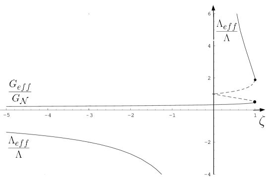
Figure 1: Plot of $\frac{\Lambda_{eff}}{\Lambda}$ and $\frac{G_{eff}}{G_{\mathcal{N}}}$ as a function of $\zeta$ for both cases “$+$” and “$-$”. The solid and dashed line correspond respectively to “$+$” and “$-$” cases. The transitions between them takes place on the filled circles.

The compatibility between Eqs. (19) and (20) implies that:

$$\varphi^{2} = \frac{1}{4\alpha_{{}_{\rm{s}}}G_{\mathcal{N}}}\Bigg{(}1\pm\sqrt{1-\zeta}\ \Bigg{)}$$ (21)

$$\zeta = 16\frac{G_{\mathcal{N}}\Lambda}{\alpha_{{}_{\rm{s}}}}$$

In the following, we will use “$+$” to indicate the positive sign solution and “$-$” for the negative sign solution of Eq. (21). Since $\varphi^{2}$ must be positive if one wants to guarantee the positive sign of $\sqrt{G}$, the ranges of the dimensionless constant $\zeta$ are $]-\infty,1]$ for the “$+$” solution and $[0,1]$ for the “$-$” one. Then $\zeta$ can be viewed as the ratio of the interaction and vacuum characteristic lengths, i.e. $\zeta=\pm 16l_{\alpha}l_{G_{\mathcal{N}}}/l_{\Lambda}$. When the compatibility condition (21) is respected, there remains the Einstein equations to be solved:

$$r_{\mu\nu}=-2\Lambda_{eff}g_{\mu\nu}$$ (22)

An effective cosmological constant, induced by YM theory and gravity,

$$\Lambda_{eff}=\Lambda\frac{2(1\pm\sqrt{1-\zeta})}{\zeta}$$ (23)

has been introduced. We have considered that $G_{\mathcal{N}}$ and $\alpha_{{}_{\rm{s}}}$ are positive quantities, therefore $\Lambda_{eff}\geq 0$ for all values of $\Lambda\leq\frac{\alpha_{{}_{\rm{s}}}}{16G_{\mathcal{N}}}$. Replacing $G_{\mu\nu}$ by its ansatz in Eq. (7) one obtains in addition to $\Lambda_{eff}$, an effective gravitational constant:

$$G_{eff}=G_{\mathcal{N}}\frac{1}{2\pm\sqrt{1-\zeta}}$$ (24)

As can be seen in figure 1, when $\zeta\in[0,1]$ the two solutions, “$-$” and “$+$” coexist. For these solutions $\Lambda$ and $\Lambda_{eff}$ are positive and the addition of the YM fields does not change the topology of space. In contrast to this, when $\zeta$ is negative, $\Lambda_{eff}$ remains positive while $\Lambda$ is negative, then the addition of the YM fields changes the topology of space from a quotient of S³ to a quotient of H³. One can note that when $\zeta\rightarrow 0$ the “$-$” solution gives

$$\Lambda_{eff}\rightarrow\Lambda\ \ ,\ \ G_{eff}\rightarrow G_{\mathcal{N}}$$

This happens when one of the length scales defined by $\alpha_{{}_{\rm{s}}}$ or $G_{\mathcal{N}}$ tends to $0$ and therefore when the two theories decouple.

To summarize, one can say that the ansatz proposed in Eq. (17) reduces the EYM equations to the Einstein equations with an effective cosmological constant (23) which in all cases is positive, corresponding to an attractive interaction, and an effective gravitational constant, (24).

When one has solved Eq. (22), one has a solution for $(g_{\mu\nu},G_{\mu\nu})$ and consequently for $(g_{\mu\nu},E^{a}_{\mu})$, where $E^{a}_{\mu}$ is defined up to an SO(3) rotation. Using Eq. (5), one obtains the YM field $A^{a}_{\mu}$ as being

$$A^{b}_{\mu}={1\over 2}\epsilon^{bcd}\big{(}E_{c}^{\nu}\partial_{\mu}E^{d}_{\nu}-E_{c}^{\nu}\Gamma^{\rho}_{\nu\mu}E^{d}_{\rho}\big{)}$$ (25)

It is interesting to note that the solutions found through this reformulation are fully non-Abelian. This can be viewed as beeing due to the absence of a Killing vector $\xi=\xi^{a}\sigma_{a}/2$ in the su(2) algebra. Such a Killing vector is defined by

$$D_{\mu}\xi=0$$

This is equivalent to $\epsilon_{abc}E^{a}_{\mu}\xi^{b}=0$. This last relation shows that $\xi$ exists if, and only if, $E^{a}_{\mu}$ is not invertible, i.e. if $\det(E)=0$. The configurations given by this reformulation are thus totally non-Abelian, which is not the case of the currently known analytical solutions.

Example of an application: Black hole solutions.

Many solutions to Eq. (22) are known but one of the most exciting ones is the BTZ black hole [8]. We will consider here the non-rotating BTZ black hole. One can extrapolate it to Euclidean time. It can be easily shown that through such a continuation, the Euclidean solution of the Einstein equations is:

$$ds^{2} = g_{\mu\nu}dx^{\mu}dx^{\nu}$$

$$= N^{2}d\tau^{2}+\frac{dr^{2}}{N^{2}}+r^{2}d\theta^{2}$$

where $N$ is a function of the radial distance “$r$” such that

$$N^{2}(r) = -8G_{eff}M_{eff}+\Lambda_{eff}r^{2}$$ (27)

Here, $M_{eff}$ is an integration constant.
The strong line element is

$$dS^{2} = G_{\mu\nu}dx^{\mu}dx^{\nu}$$

$$= \varphi^{4}(N^{2}d\tau^{2}+\frac{dr^{2}}{N^{2}}+r^{2}d\theta^{2})$$

and corresponds equally to the BTZ line element in the dilated space coordinate $dT=\varphi^{2}d\tau,dR=\varphi^{2}dr,d\Theta=d\theta$. As for the BTZ black hole solution, the line element, Eq. (Einstein-Yang-Mills black hole solutions in three dimensions.) has apparent singularities at

$$r_{s}=\left(\frac{8G_{eff}M_{eff}}{\Lambda_{eff}}\right)^{1/2}$$ (29)

As can be seen in figure 1, for fixed $\zeta>0$ and fixed positive $M_{eff}$ there are two black holes, a large one corresponding to the “$-$” solution in Eq. (21) and a smaller one corresponding to the “$+$” solution. Both of these black holes have a radius smaller than the vacuum BTZ black hole. This can be interpreted by the fact that in this regime both the universal and strong gravities are attractive.
For fixed $\zeta<0$ there is only one black hole. In this case, strong gravity is attractive while universal gravity is repulsive but strong gravity wins and black holes can appear.

Yang-Mills fields.

We will now show the YM fields corresponding to the strong metric, Eq. (Einstein-Yang-Mills black hole solutions in three dimensions.). This strong metric can be built from the particular triad field:

$$\mu=\begin{array}[]{ccc}0,&1,&2\end{array}\hskip 11.38109pt$$ (31)

$${{E^{a}_{\mu}}^{{}^{{}^{o}}}}=\frac{2\Lambda_{eff}}{\alpha_{{}_{\rm{s}}}^{2}}\left(\begin{array}[]{ccc}N&0&0\\ 0&\frac{1}{N}&0\\ 0&0&r\end{array}\right) \begin{array}[]{c}a=1\\ a=2\\ a=3\end{array}$$ (38)

However, when we decompose the strong metric, Eq. (3) into a triad field we introduce a gauge choice in a gauge invariant formalism. The most general triad solution to our problem is

$$E^{a}_{\mu}=\Omega^{-1}{{E^{a}_{\mu}}^{{}^{{}^{o}}}}{\hskip 8.82036pt\Omega}$$

where $\Omega$ is any SU(2)/${\mathbb{Z}}_{2}$ valued function. Inserting Eq. (31) into Eq. (25) and keeping the same conventions for the matrices, one obtains:

$${{A^{b}_{\mu}}^{{}^{\vspace{2mm}o}}}\hskip 8.82036pt=\left(\begin{array}[]{ccc}0&0&-N\\ 0&0&0\\ NN^{\prime}&0&0\end{array}\right)$$ (42)

where $N^{\prime}$ represents the derivation of $N$ with respect to $r$. Taking Eq. (27) into account this reduces to

$${{A^{b}_{\mu}}^{{}^{\vspace{2mm}o}}}\hskip 8.82036pt=\left(\begin{array}[]{ccc}0&0&-N\\ 0&0&0\\ \Lambda_{eff}r&0&0\end{array}\right)$$ (46)

This result can be rewritten in the gauge algebra as:

$$A^{{}^{{}^{o}}}\hskip 2.84526pt\equiv {{A^{b}_{\mu}}^{{}^{\vspace{2mm}o}}}\hskip 8.82036pt\frac{\sigma_{b}}{2}dx^{\mu}$$ (47)

$$=\left(\begin{array}[]{cc}r\Lambda_{eff}d\tau&-Nd\theta\\ &\\ -Nd\theta&-r\Lambda_{eff}d\tau\end{array}\right)$$ (51)

where $\sigma_{b}$ are the Pauli matrices:

$$\sigma_{1}=\left(\begin{array}[]{cc}0&1\\ 1&0\end{array}\right) \sigma_{2}=\left(\begin{array}[]{cc}0&-i\\ i&0\end{array}\right) \sigma_{3}=\left(\begin{array}[]{cc}1&0\\ 0&-1\end{array}\right)$$ (58)

In the same way as for ${{E^{a}_{\mu}}^{{}^{{}^{o}}}}\$, the solution $A^{{}^{{}^{o}}}$ can be extended to

$$A=\Omega^{-1}A^{{}^{{}^{o}}}\hskip 8.53581pt\Omega+i\Omega^{-1}\partial_{\mu}\Omega$$

Note that all the possible solutions of $A$ are classified by the homotopy classes of the applications $\Omega:{\mathcal{M}}\rightarrow{\mathrm{S}O(3)}$. In thermodynamical applications, time is “compactified” and the interior region has to be removed in such a way that the topology of ${\mathcal{M}}$ reduces to the empty torus. Finally, the possible solutions for the potential, $A$, are classified by the homotopy classes of $\Omega:S^{1}\times S^{1}\rightarrow{\mathrm{S}O(3)}$.

Energy and mass.

In this section the energy and the mass of the black holes found before are given. We will use the quasi-local formalism of [9], specially extended in [10] to the case of the BTZ black hole. This formalism is powerful because it can be applied in a bounded, finite spatial region, with no assumptions on the asymptotic flatness of space-time. It is based on a Hamilton-Jacobi treatment of the gravitational action, Eq. (7) with its boundary term

$$S_{B}=\frac{1}{8\pi G_{\mathcal{N}}}\int_{\Sigma_{t^{\prime}}\cup\Sigma_{t^{\prime\prime}}}{d^{2}x\sqrt{h}K}-\frac{1}{8\pi G_{\mathcal{N}}}\int_{\mathcal{B}}{d^{2}x\sqrt{-\gamma}\Theta}$$

In this equation $\Sigma_{t}$ is a space-like hyper-surface defined by $t=$constant and $r\leq R$, $\mathcal{B}$ is the surface defined by $t^{\prime}\leq t\leq t^{\prime\prime}$ and $r=R$. $h_{ij}$ and $\gamma_{ij}$ are respectively the metrics on $\Sigma$ and $\mathcal{B}$ with external curvatures $K$ and $\Theta$. For a given solution one varies this action but leaves the metric on the boundaries free. In this case one obtains

$$\delta S=\delta S_{\mathrm{Y}M}+\int_{\Sigma_{t^{\prime}}\cup\Sigma_{t^{\prime\prime}}}{d^{2}xP^{ij}\delta h_{ij}}+\int_{\mathcal{B}}{d^{2}x\pi^{ij}\delta\gamma_{ij}}$$

where $P_{ij}$ is the gravitational momentum associated with the space-like hyper-surface $\Sigma$ and $\pi_{ij}$ the gravitational momentum on $\mathcal{B}$. This last momentum can be interpreted as a quasi-conserved energy-momentum tensor on $\mathcal{B}$. Selecting its normal-normal, normal-parallel and parallel-parallel components one can extract the quasi-local energy $\epsilon$, the angular momentum $J_{\theta}$ and the stress $s^{\theta\theta}$. All these quantities are defined up to an additive constant because one can always add on a boundary action $S^{0}$ to $S$. This procedure fixes the zero energy point. Finally, if we apply this formalism to the Minkowskian continuation of our metric, one has [10]

$$\epsilon = \frac{\sigma^{\theta\theta}k_{\theta\theta}}{8\pi G_{\mathcal{N}}}-\epsilon_{0}$$ (59)

$$\j_{\theta} = 0$$ (60)

$$\sigma_{\theta\theta}s^{\theta\theta} = -\frac{1}{8\pi G_{\mathcal{N}}}n_{\mu}a^{\mu}-\frac{\partial R\epsilon_{0}}{\partial R}$$ (61)

where $\sigma_{\theta\theta}=R^{2}$ is the metric on $B=\partial\Sigma$, $k_{\theta\theta}=-RN$ is the extrinsic curvature of $B$, $\hat{n}$ is the normal vector of $\mathcal{B}$ and $a^{\mu}$ is the acceleration of $B$. The choice of the subtraction term $\epsilon_{0}$ poses a problem. In the range $\zeta\in[0,1]$ it is possible to take the empty anti-De Sitter (aDS) space-time as a reference but it is no longer possible in the range $\zeta\in]-\infty,0[$ where the empty space-time is De Sitter and where the energy is not defined beyond the cosmological horizon.

In the case where $\Lambda>0$, if one takes as a reference the space-time metric of the empty aDS space-time, then the total internal energy is

$$E = \int_{B}{d\theta\sqrt{\sigma}\epsilon}$$

$$= -\frac{1}{4G_{\mathcal{N}}}\Big{(}\sqrt{-8M_{eff}G_{eff}+\Lambda_{eff}R^{2}}-\sqrt{1+\Lambda R^{2}}\Big{)}\ ,$$

which diverges when $R\rightarrow\infty$, we then have

$$E\sim-\frac{1}{4G_{\mathcal{N}}}\Big{(}\sqrt{\Lambda_{eff}}-\sqrt{\Lambda}\Big{)}R$$

This infinity shows that our solution considerably changes the structure of space-time. Alternatively, if one wants a correctly referenced space-time for all values of $\zeta$ one has to take the aDS space-time defined by $\Lambda_{eff}$. Then for all $\zeta$,

$$E = -\frac{1}{4G_{\mathcal{N}}}\Big{(}\sqrt{-8M_{eff}G_{eff}+\Lambda_{eff}R^{2}}-\sqrt{1+\Lambda_{eff}R^{2}}\Big{)}\ ,$$

which tends to zero as $R$ tends to infinity. The stress $\sigma_{\theta\theta}s^{\theta\theta}$ is proportional to the thermodynamical “surface” pressure on the 1-dimensional “surface” $B$:

$$\sigma_{\theta\theta}s^{\theta\theta}=-\frac{1}{8\pi G_{\mathcal{N}}}(N^{\prime}(R)-N_{0}^{\prime}(R))$$

where the $N^{\prime}$ denotes the derivation of $N$ with respect to $R$ and where $N_{0}$ is the subtraction term $\sqrt{1+\Lambda_{0}R^{2}}$ with $\Lambda_{0}=\Lambda$ or $\Lambda_{eff}$ depending on the background choice. This “surface” pressure goes as

$$\sigma_{\theta\theta}s^{\theta\theta}\sim_{{}_{R\rightarrow\infty}} -\frac{1}{8\pi G_{\mathcal{N}}}(\sqrt{\Lambda_{eff}}-\sqrt{\Lambda_{0}})$$

In the quasi-local formalism, the conserved mass is not equivalent to energy in an asymptotically non-flat space-time. It is associated with the conserved charge of the time-like Killing vector and is thus ([10])

$$M = \int_{B}{d\theta\sqrt{\sigma}N\epsilon}$$

$$= -\frac{N(N-N_{0})}{4G_{\mathcal{N}}}$$

and with our choice, $\Lambda_{0}=\Lambda_{eff}$, this goes as

$$M \sim_{{}_{R\rightarrow\infty}} \frac{M_{eff}G_{eff}-1}{G_{\mathcal{N}}}$$

This last value gives the pure gravitational mass of the black hole.

Conclusions and outlook.

In the previous sections we have developed a new method for finding solutions to the 3-d Euclidean EYM equations. The crux of this method is the use of a reformulated YM theory as a gravitational theory. The present reformulation suggests many ans tze. We have studied the simplest one based on a conformal link between the strong and the true metric. This ansatz is exactly solvable for the YM field when one has a solution to the Einstein equations.

The ansatz gives some positive results: the solutions of EYM are explicit, they are fully non-Abelian, they reveal a rich topological structure of EYM space due to a non-trivial mapping between the base space and the gauge group. It is possible that this topological structure is linked with the classification of the usual EYM black holes by a set of integer numbers [1].

Unfortunately, this ansatz is very rough and it leads to a bad asymptotic behaviour for the YM field. In the case of the black hole solutions, we have found that the bad behaviour of the YM fields greatly changes the topology of space. For this reason, it is not possible in the case where $\Lambda<0$ to choose the vacuum De Sitter space as a reference space. When $\Lambda\geq 0$, the topology of space remains unchanged and it is, in principle, possible to take an aDS space as a reference. However, due to the shift from $\Lambda$ to $\Lambda_{eff}$, all the quantities obtained in this case are infinite. This point is not yet physically understood. Nevertheless, it is possible to begin a study of the thermodynamical quantities of these black holes using Eq. (Einstein-Yang-Mills black hole solutions in three dimensions.) and those thereafter. The charge of the black hole is still unclear [15] and so we have not included it in this discussion.

The bad behaviour of the YM fields can be cured in extended ans tze. The conformal ansatz considered here belongs to the large ensemble where the two metrics are related by a general transformation $A$:

$$G_{\mu\nu}(x)=A^{\rho}_{\mu}(x)g_{\rho\sigma}(x)A^{\sigma}_{\nu}(x)$$

One could constrain $A$ by requiring a good asymptotic behaviour.

Many other extensions are possible. We have applied our ansatz to a BTZ black hole, but this can be easily extended to all vacuum solutions of the Euclidean Einstein equations in three dimensions such as multi-black hole solutions [14]. Moreover, as our procedure systematically eliminates the gauge connection of the equations of motion, one can include various other fields such has dilaton, electro-magnetic, etc. The inclusion of other fields directly coupled to gauge fields, such as quark fields, is more difficult but possible in the framework of the ansatz. At the moment, this reformulation is well defined only in three dimensions with a gauge group SU(2). It is however possible to easily include matter sources which will give torsion and a topological term to the YM theory which will in turn give a strong gravitational topological term. It is important to be assured that the reformulation is not an accident of SU(2) gauge theories in three dimensions. It is in fact possible to extend this reformulation to the SU(N) gauge group in three dimensions but the result is already rather complicated for SU(3). There are also some possibilities for reformulating in 2 and 4 dimensions [13].

Acknowledgments
I want to thank in particular M. Bauer for the stimulating discussions we had and all his explanations necessary to this article. It is a pleasure to thank G. Cohen-Tannoudji for his advice and critical reading, M. Knecht, G. Clement and S.deser for their remarks, M. Mac Cormick for her corrections and I. Porto-Cavalcante and D. Lhuillier for their stimulating discussions.

References

-
[1]
R. Bartnik, J. McKinnon, Phys. Rev. Lett. 61 (1988) 141.
D.V. Gal’tsov, E.E. Donets, M.Yu. Zotov, Pis’ma Zh. Eksp. Teor. Fiz. 65 (1997)855 (GR-QC 9706063) -
[2]
S. Deser, R. Jackiw, G. ’t Hooft, Ann. Phys. 152 (1984) 220
S. Deser, R. Jackiw, Ann. Phys. 153 (1984) 405 - [3] A. Achùcarro, P.K. Townsend, Phys. Lett. 180B (1986), 89
- [4] E. Witten, Nucl. Phys. B311(1988) 46
- [5] A. Ashtekar, Phys.Rev.Lett. 77 (1996) 4864-4867
-
[6]
J.B. Hartle, S.W. Hawking, Phys. Rev. D28 (1983) 2960.
G.W. Gibbons, S.W. Hawking, Phys. Rev. D15(1977) 2752 - [7] F.A. Lunev, Phys. Lett B295 (1992) 99.
-
[8]
M. Bañados, C. Teitelboim, Zanelli, J. Phys. Rev. Lett 69 (1992) 1849.
M. Bañados, M. Henneaux,C. Teitelboim, J. Zanelli, Phys. Rev. D48 (1993) 1506. - [9] J.D. Brown, J.W. York, Phys. Rev.D47 (1993)1407
- [10] J.D. Brown, J. Creighton, R.B. Mann, Phys. Rev.D50 (1994) 6394
- [11] F.A. Lunev, O.V. Pavlovskii, Singular solutions of Yang-Mills equations and bag model. hep-ph/9609452
- [12] A. Actor, Rev. Mod. Phys. 51 (1979) 461
- [13] F.A. Lunev, J. Math. Phys. 37(1996)5351
- [14] G. Clément, Phys. Rev. D50 (1994) 7119
- [15] G. Clément, Private communication.