DILATONIC GLOBAL STRINGS

Abstract

We examine the field equations of a self-gravitating global string in low energy superstring gravity, allowing for an arbitrary coupling of the global string to the dilaton. Massive and massless dilatons are considered. For the massive dilaton the spacetime is similar to the recently discovered non-singular time-dependent Einstein self-gravitating global string, but the massless dilaton generically gives a singular spacetime, even allowing for time-dependence. We also demonstrate a time-dependent non-singular string/anti-string configuration, in which the string pair causes a compactification of two of the spatial dimensions, albeit on a very large scale.

I Introduction

Topological defects crop up widely in physics; in cosmology they have been put forward as a possible source for the density perturbations which seeded galaxy formation [2]. Phase transitions in the early universe can give rise to various forms of topological defect. A defect is a discontinuity in the vacuum and is classified according to the topology of the vacuum manifold of the field theory model being used. Disconnected vacuum manifolds give domain walls, non-simply connected manifolds, strings, and vacuum manifolds with non-contractible spheres give monopoles. Strings and monopoles can be further divided into local and global defects depending on the nature of the symmetry broken. Local defects are formed when the symmetry broken is gauged, and the Higgs mechanism typically removes any Goldstone bosons, meaning that the defect has a well-defined core and finite energy per unit defect area. Global defects on the other hand (with the exception of the domain wall which does not result from the breaking of a continuous symmetry) typically have a residual Goldstone field in the Lagrangian, which translates to a power law fall-off in the core energy density and a divergent total energy. More unusual defects, such as semi-local strings [3] also exist, but we do not consider these here.

Given this difference between local and global defects, we might expect them to have significantly different behaviour, and this is particularly evident in their coupling to gravity. Whilst local strings [4] and monopoles [5] are well-behaved and asymptote flat or locally flat spacetimes, global strings [6, 7] and monopoles [8, 9] have strong effects at large distances. Indeed, the spacetime of a global string was for some time thought to be singular [6]. In fact, the spacetime is time-dependent [7] with a de-Sitter expansion along the spatial extent of the defect. The spacetime is also characterised by an event horizon at a finite distance from the string core, although this horizon appears to be unstable to perturbations [10]. Of course, this work has all been performed within the context of general relativity. At sufficiently high energy scales it seems likely that gravity is not given by the Einstein action, but becomes modified, for example, by superstring terms which are scalar-tensor in nature [11]. Low energy string gravity is reminiscent of the scalar-tensor theories of Jordan, Brans and Dicke [12], and is equivalent to Brans-Dicke theory for a particular value of the Brans-Dicke parameter : $\omega=-1$. The implications of Brans-Dicke gravity for defects have been explored for local strings [13] and global monopoles [14]. However, since the Brans-Dicke parameter is known to be constrained by $\omega>500$ [15], we are more interested in exploring the low energy superstring action, particularly with a massive dilaton, although massless dilatons will provide a comparison with Brans-Dicke results. Moreover, some recent superstring inspired models of inflation [16] appear to allow for cosmic string defects to form of either the local or global variety, therefore it is useful to know how these objects interact with the dilaton.

In this paper we will consider the implications of superstring gravity for global cosmic strings. In particular we will address the question of whether a non-singular spacetime exists for the string. Recently Sen et. al. [17] studied global strings in Brans-Dicke theory. We disagree with their claim that a static, non-singular solution exists for the string spacetime. The structure of this paper is as follows. First, we briefly review the global string in Einstein gravity. We then study the global string in superstring gravity, for both massless and massive dilatons. Finally, we compare our results with the literature and present our conclusions - in particular, we present a novel solution which represents a self-gravitating string/anti-string pair on a closed two-dimensional spatial section.

II Non-static strings in Einstein gravity

In this section, we review the global string in Einstein gravity. The Lagrangian for an isolated $U(1)$ global string is

$${\mathcal{L}}=\left(\nabla_{a}\Phi\right)^{\dagger}\nabla^{a}\Phi-\frac{\lambda}{4}\left(\Phi^{\dagger}\Phi-\eta^{2}\right)^{2}$$ (1)

By writing

$$\Phi=\eta Xe^{i\chi}$$ (2)

we reformulate the complex scalar field into two real, interacting scalar fields, one massive ($X$), the other a massless Goldstone boson ($\chi$)

$${\mathcal{L}}=\eta^{2}(\nabla_{a}X)^{2}+\eta^{2}X^{2}(\nabla_{a}\chi)^{2}-\frac{\lambda\eta^{4}}{4}(X^{2}-1)^{2}$$ (3)

A vortex solution is characterised by the existence of closed loops in space for which

$$\frac{1}{2\pi}\oint\frac{d\chi}{dl}dl=n\in Z\hskip-8.53581ptZ$$ (4)

We take the winding number $n=1$ and look for a solution describing an infinitely long, isolated, straight string. The string spacetime is expected to exhibit cylindrical symmetry. If, in addition, we require the string to have fixed proper width, it can be shown [7] that coordinates may be chosen in which the metric is

$$ds^{2}=e^{2A(r)}\left(dt^{2}-e^{2b(t)}dz^{2}\right)-dr^{2}-C^{2}(r)d\theta^{2}$$ (5)

where $\chi=\theta$, and $X=X(r)$.

Since we are dealing with an isolated global string, for convenience we set $\sqrt{\lambda}\eta=1$, choosing units in which the string width is $O(1)$. Then the Einstein equations become

$$A^{\prime\prime}+\frac{C^{\prime\prime}}{C}+A^{\prime 2}+\frac{A^{\prime}C^{\prime}}{C} = -\epsilon\hat{T}_{t}^{t}$$ (6)

$$(\ddot{b}+\dot{b}^{2})e^{-2A}-A^{\prime 2}-2\frac{A^{\prime}C^{\prime}}{C} = \epsilon\hat{T}_{r}^{r}$$ (7)

$$(\ddot{b}+\dot{b}^{2})e^{-2A}-2A^{\prime\prime}-3A^{\prime 2} = \epsilon\hat{T}_{\theta}^{\theta}$$ (8)

where $\epsilon=8\pi G\eta^{2}$ measures the gravitational strength of the string, and $\epsilon{\hat{T}}_{ab}=8\pi GT_{ab}$. In addition, the field equation for $X$ is

$$-X^{\prime\prime}-\left(\frac{C^{\prime}}{C}+2A^{\prime}\right)X^{\prime}+\frac{X}{C^{2}}+\textstyle{1\over 2}X(X^{2}-1)=0$$ (9)

Clearly (7) and (8) require

$$\ddot{b}+\dot{b}^{2}=b_{0}$$ (10)

where $b_{0}$ is a constant. Reference [7] examined the behaviour of the string metric for different values of the free parameter $b_{0}$. This analysis is involved and will largely be mirrored in the next section; therefore we will merely sketch the results. The region of parameter space $b_{0}\leq 0$ is excluded as the metric can be proved to be singular in this case. For $b_{0}>0$ it can be shown that for a non-singular isolated string solution to exist, $e^{2A}\rightarrow 0$ at some finite $r_{0}$. This $r_{0}$ would represent an event horizon for the global string spacetime, analogous to that of the domain wall [18]. The asymptotic metric near this point would be

$$ds^{2}\simeq b_{0}(r_{0}-r)^{2}\left[dt^{2}-\cosh^{2}\sqrt{b_{0}}tdz^{2}\right]-dr^{2}-C_{0}^{2}d\theta^{2}$$ (11)

for some constant $C_{0}$. The curvature invariants for this metric are all finite, and a coordinate system can be found which extends beyond the event horizon $r=r_{0}$, verifying the coordinate nature of the singularity.

Of course, we have not shown such a non-singular solution necessarily exists. However, as demonstrated in [7], we can reduce the far-field equations describing the global string metric to a two-dimensional dynamical system. Whether or not (11) is admissible as an asymptotic solution for the global string reduces to the question of whether the dynamical system will asymptote the solution appropriate to (11) in phase space. By integrating out the full equations of motion to the edge of the vortex to find initial conditions for the dynamical system, it can indeed be shown that there always exists a $b_{0}$ for which a trajectory interpolates between the initial conditions and the asymptotic solution (11).

III Dilaton gravity and global strings

We are interested in the behaviour of the global string metric when gravitational interactions take a form typical of low energy string theory. In its minimal form, string gravity replaces the gravitational constant, $G$, by a scalar field, the dilaton. To account for the unknown coupling of the dilaton to the global string, we choose the action

$$S=\int d^{4}x\sqrt{-\hat{g}}\left[e^{-2\phi}\left(-\hat{R}-4(\hat{\nabla}\phi)^{2}-\hat{V}(\phi)\right)+e^{2a\phi}{\mathcal{L}}\right]$$ (12)

where $\mathcal{L}$ is as in (1). The potential for the dilaton ${\hat{V}}(\phi)$ is for the moment assumed general. This action is written in terms of the string metric which appears in the string sigma model. To facilitate comparison with the previous section we instead choose to write the action in the Einstein frame, which is related to the string frame via the conformal transformation

$$g_{ab}=e^{-2\phi}\hat{g}_{ab}$$ (13)

in which the gravitational part of the action appears in the normal Einstein form

$$S=\int d^{4}x\sqrt{-g}\left[-R+2(\nabla\phi)^{2}-V(\phi)+e^{2(a+2)\phi}{\mathcal{L}}(\Phi,e^{2\phi}g)\right]$$ (14)

where $V(\phi)=e^{2\phi}\hat{V}(\phi)$. The energy-momentum tensor is now

$$T_{ab} = e^{2(a+2)\phi}\left[\frac{\delta{\mathcal{L}}(\Phi,e^{2\phi}g)}{\delta g^{ab}}-\textstyle{1\over 2}g_{ab}{\mathcal{L}}(\Phi,e^{2\phi}g)\right]$$ (15)

$$= {\eta^{2}\over 2}e^{2(a+1)\phi}\left[2\nabla_{a}X\nabla_{b}X+2X^{2}\nabla_{a}\theta\nabla_{b}\theta-g_{ab}\left((\nabla X)^{2}+X^{2}(\nabla\theta)^{2}-{e^{2\phi}\over 4}(X^{2}-1)^{2}\right)\right]$$ (16)

where $\Phi$ takes the form (2) and $\chi=\theta$ as before. Einstein’s equation becomes

$$G_{ab}=\epsilon{\hat{T}}_{ab}+S_{ab}$$ (17)

where ${\hat{T}}_{ab}$ is defined as before, and $\epsilon=\eta^{2}/2$. The second term, $S_{ab}$, represents the energy-momentum of the dilaton

$$S_{ab}=2\nabla_{a}\phi\nabla_{b}\phi+\frac{1}{2}g_{ab}V(\phi)-g_{ab}(\nabla\phi)^{2}$$ (18)

which has as its equation of motion

$$-\Box\phi=\frac{1}{4}\frac{\partial V}{\partial\phi}+\epsilon(a+1)\hat{T}_{t}^{t}+\textstyle{1\over 4}\epsilon e^{2(a+2)\phi}(X^{2}-1)^{2}$$ (19)

We will take a quadratic approximation $V(\phi)=2M^{2}\phi^{2}$ (where the mass $M$ is measured in units of the Higgs mass) which will only be valid for small $\phi$ when $M\neq 0$ – an approximation which will require justification at the appropriate stage. Note that we are ruling out a linear or exponential potential which would correspond to a cosmological constant in the string frame. In practise, we expect $10^{-12}<M<1$, corresponding to a dilaton mass in the range 1 TeV – 10¹⁵GeV. A dilaton with a lower mass than 1TeV would appear to be ruled out and a higher mass dilaton would give a de facto Einstein gravitating global string.

As in Section 2, we choose the general, time-dependent, cylindrically symmetric metric compatible with the symmetries of the source. That is

$$ds^{2}=e^{2A(r)}\left(dt^{2}-e^{2b(t)}dz^{2}\right)-dr^{2}-C^{2}(r)d\theta^{2}$$ (20)

where $b$ can be shown to satisfy (10) as before. Taking $\sqrt{\lambda}\eta=1$, the rescaled, modified energy-momentum tensor is now

$$\hat{T}_{t}^{t}=\hat{T}_{z}^{z} = e^{2(a+2)\phi}\left(e^{-2\phi}\left(X^{\prime 2}+\frac{X^{2}}{C^{2}}\right)+\textstyle{1\over 4}(X^{2}-1)^{2}\right)$$ (21)

$$\hat{T}_{r}^{r} = e^{2(a+2)\phi}\left(e^{-2\phi}\left(-X^{\prime 2}+\frac{X^{2}}{C^{2}}\right)+\textstyle{1\over 4}(X^{2}-1)^{2}\right)$$ (22)

$$\hat{T}_{\theta}^{\theta} = e^{2(a+2)\phi}\left(e^{-2\phi}\left(X^{\prime 2}-\frac{X^{2}}{C^{2}}\right)+\textstyle{1\over 4}(X^{2}-1)^{2}\right)$$ (23)

and the equation of motion for $X$ is

$$\left[Ce^{2A}e^{2(a+1)\phi}X^{\prime}\right]^{\prime}=\frac{X}{C}e^{2A}e^{2(a+1)\phi}+\textstyle{1\over 2}Ce^{2A}e^{2(a+2)\phi}X(X^{2}-1)$$ (24)

The gravi-dilaton equations are given explicitly by

$$\left[C^{\prime}e^{2A}\right]^{\prime} = -\epsilon Ce^{2A}e^{2(a+1)\phi}\left(\frac{2X^{2}}{C^{2}}+\textstyle{1\over 4}e^{2\phi}(X^{2}-1)^{2}\right)-M^{2}Ce^{2A}\phi^{2}$$ (25)

$$\left[A^{\prime}Ce^{2A}\right]^{\prime} = C\left(b_{0}-\textstyle{1\over 4}\epsilon e^{2A}e^{2(a+2)\phi}(X^{2}-1)^{2}\right)-M^{2}Ce^{2A}\phi^{2}$$ (26)

$$A^{\prime 2}+\frac{2A^{\prime}C^{\prime}}{C} = b_{0}e^{-2A}+\phi^{\prime 2}-M^{2}\phi^{2}-\epsilon e^{2(a+1)\phi}\left(-{X^{\prime}}^{2}+\frac{X^{2}}{C^{2}}+\textstyle{1\over 4}e^{2\phi}(X^{2}-1)^{2}\right)$$ (27)

$$\left[Ce^{2A}\phi^{\prime}\right]^{\prime} = M^{2}Ce^{2A}\phi+\epsilon Ce^{2A}e^{2(a+1)\phi}\left((a+1)\left(X^{\prime 2}+\frac{X^{2}}{C^{2}}\right)+\frac{(a+2)e^{2\phi}}{4}(X^{2}-1)^{2}\right)$$ (28)

Having set up the formalism and equations of motion, we now turn to analyzing the possible solutions.

A Preliminary remarks

We wish to examine under what conditions the spacetime of a global string may be non-singular. We consider in turn the two cases $b_{0}\leq 0$ and $b_{0}>0$.

1 $b_{0}\leq 0$

We now prove that if $b_{0}\leq 0$ alll solutions are singular. Note that (25) and (26) imply

$$\left[Ce^{2A}\right]^{\prime\prime}=2b_{0}C-\epsilon Ce^{2A}e^{2(a+1)\phi}\left(\frac{2X^{2}}{C^{2}}+\frac{3}{4}e^{2\phi}(X^{2}-1)^{2}\right)-3M^{2}Ce^{2A}\phi^{2}\leq 0$$ (29)

Thus $Ce^{2A}\leq r$ for all $r$. Now if $(Ce^{2A})^{\prime}=0$ at any point then (29) implies $Ce^{2A}\rightarrow 0$ at some $r_{0}$ with $(Ce^{2A})^{\prime}$ strictly negative. Then

$$\frac{(Ce^{2A})^{\prime}}{Ce^{2A}}=2A^{\prime}+\frac{C^{\prime}}{C}\rightarrow-\infty$$ (30)

as $r\rightarrow r_{0}$. Now (26) implies $A^{\prime}$ is strictly negative away from $r=0$. So either $A^{\prime}C^{\prime}/C$ or $A^{\prime}$ becomes infinite at $r_{0}$. But then

$$R_{abcd}^{2}\propto\left(\frac{C^{\prime\prime}}{C}\right)^{2}+2\left(\frac{A^{\prime}C^{\prime}}{C}\right)^{2}+2(A^{\prime\prime}+A^{\prime 2})^{2}+(A^{\prime 2}-b_{0}e^{-2A})^{2}$$ (31)

would become infinite at $r_{0}$ indicating a physical singularity. So for a non-singular spacetime, we take $(Ce^{2A})^{\prime}>0$.

Define

$$\alpha_{1}(r) = \epsilon\int_{0}^{r}\frac{e^{2A}e^{2(a+1)\phi}X^{2}}{C}dr$$ (32)

$$\alpha_{2}(r) = \epsilon\int_{0}^{r}\textstyle{1\over 4}Ce^{2A}e^{2(a+2)\phi}(X^{2}-1)^{2}dr$$ (33)

$$\alpha_{3}(r) = |b_{0}|\int_{0}^{r}Cdr$$ (34)

$$\alpha_{4}(r) = \epsilon\int_{0}^{r}Ce^{2A}e^{2(a+1)\phi}X^{\prime 2}dr$$ (35)

$$\alpha_{5}(r) = M^{2}\int_{0}^{r}Ce^{2A}\phi^{2}dr$$ (36)

Then positivity of $(Ce^{2A})^{\prime}$ implies

$$1>2\alpha_{1}(r)+3\alpha_{2}(r)+2\alpha_{3}(r)+3\alpha_{5}(r)$$ (37)

for all $r$, hence the $\alpha_{i}$ (i = 1,2,3,5) are bounded. But since $A^{\prime}$ is negative and $(Ce^{2A})^{\prime}$ positive, $C^{\prime}$ must be greater than zero for all $r$. Hence $\int C$ cannot converge and the spacetime must be singular for $b_{0}<0$.

For $b_{0}=0$, note that convergence of an $\alpha_{i}$ implies that its integrand, $I_{i}$ must be o(${1\over r}$), so $Ce^{2A}I_{i}<rI_{i}\to 0$ as $r\to\infty$. Thus as $r\to\infty$ the constraint equation (27) becomes

$$(\alpha_{2}+\alpha_{5})^{2}-2(\alpha_{2}+\alpha_{5})(1-2\alpha_{1}-\alpha_{2}-\alpha_{5})\simeq(Ce^{2A}\phi^{\prime})^{2}+Ce^{2A}I_{4}>0$$ (38)

Irrespective of the behaviour of $I_{4}$ and $\phi^{\prime}$, we see that this requires

$$3(\alpha_{2}+\alpha_{5})+4\alpha_{1}>2$$ (39)

Rearranging (37) shows that

$$3(\alpha_{2}+\alpha_{5})+4\alpha_{1}<2-3(\alpha_{2}+\alpha_{5})$$ (40)

Hence we have a contradiction, and are forced to conclude that whether the dilaton is massless or massive, no non-singular solution exists for $b_{0}\leq 0$.

Note that this argument does not use the specifics of the global string source, it simply uses the negativity of $A^{\prime}$. This is a consequence of the fact that ($T^{r}_{r}+T^{\theta}_{\theta}$) is positive, a general feature of global defects.

2 $b_{0}>0$

For $b_{0}>0$, $(A^{\prime}Ce^{2A})^{\prime}$ no longer has a definite sign and the arguments of the previous subsection will not work. We start by noting that (25) implies $(C^{\prime}e^{2A})^{\prime}\leq 0$ and hence $C^{\prime}e^{2A}\leq 1$. Either $C^{\prime}e^{2A}$ remains positive, or it does not. However, if $C^{\prime}e^{2A}>0$ for all $r$, then $\alpha_{3}(r)$ will diverge, implying that $e^{2A}\to\infty$ as $r\to\infty$. An examination of (25,26) shows that

$$C\to C_{0}\;\;\;,\;\;\;\;e^{A}\sim\sqrt{b_{0}}r\;\;\;{\rm as}\;\;\;r\to\infty$$ (41)

If $M^{2}\neq 0$, then finiteness of $\alpha_{5}$ requires $\phi\to 0$ at large $r$, and finiteness of $\alpha_{1}$ and $\alpha_{2}$ then requires $X\to 0$ and $X\to 1$ respectively - clearly an impossibility. If $M^{2}=0$, then finiteness of $\alpha_{1}$ and $\alpha_{2}$ requires

$$e^{2(a+1)\phi}X^{2} = o(1/r^{3})$$ (42)

$$e^{2(a+2)\phi}(X^{2}-1)^{2} = o(1/r^{3})$$ (43)

and so either $e^{2(a+1)\phi}=o(1/r^{3})$ or $e^{2(a+2)\phi}=o(1/r^{3})$ or both. Thus $|\phi|\rightarrow\infty$ as $r\rightarrow\infty$. But (28) shows that either $\phi$ is bounded or $(a+1)\phi\to\infty$, hence $X^{2},e^{2(a+2)\phi}=o(1/r^{3})$ as $r\to\infty$. But these are contradictory statements, since if $X$ is so bounded, the integral $\alpha_{4}$ involving $X^{\prime}$ can never diverge. Thus at some $r_{0}$, $C^{\prime}e^{2A}=0$.

Suppose that $C^{\prime}=0$ but $e^{2A}\neq 0$. Then (25) implies $C^{\prime\prime}<0$, so $C^{\prime}$ becomes negative and must remain negative. Now if $C\to 0$ at $r_{1}$, say, then non-singularity of the spacetime from (31) requires that $C^{\prime\prime},A^{\prime}\to 0$. If we require the global string to be isolated, $X\approx 1$, and hence from (25), $e^{2(a+1)\phi}\to 0$. But then integrating (28) shows $Ce^{2A}\phi^{\prime}=O(r_{1}-r)^{2}$ which means that $\phi(r_{1})$ is bounded - a contradiction. If we drop the requirement that $X\approx 1$ then we have the interesting possibility that $X\to 0$ and there is an anti-string at $C=0$. We will explore this further in the final section.

For a non-singular, isolated string solution, we require $e^{2A}\to 0$ as $r\to r_{0}$. Near this point the asymptotic solution for the metric is

$$e^{A} \sim \sqrt{b_{0}}(r_{0}-r)$$ (44)

$$C = C_{0}+O(r_{0}-r)^{2}$$ (45)

which is the event horizon discussed in [7]. The value of $b_{0}$ may be implicitly determined via integration of (26) which yields

$$\alpha_{3}=\alpha_{2}+\alpha_{5}$$ (46)

for which a linearized argument would give $b_{0}=O(\epsilon e^{1/\epsilon})$, but a more general argument [7] can certainly bound $b_{0}$ by $\epsilon^{2}$.

If the dilaton is massless we can integrate the dilaton equation (28) out to $r_{0}$ and obtain

$$Ce^{2A}\phi^{\prime}|_{r_{0}}=(a+1)\left(\alpha_{1}(r_{0})+\alpha_{4}(r_{0})\right)+(a+2)\alpha_{2}(r_{0})$$ (47)

Since nonsingularity of $R_{ab}^{2}$ requires that $\phi^{\prime}$ is finite at $r_{0}$, the LHS is zero and hence $a\in(-2,-1)$.

Of course, so far, we have merely restricted the parameter ranges in which it may be possible to find a non-singular solution. That is, $b_{0}>0$, and $-1>a>-2$ if $M^{2}=0$. It remains to be shown that such a solution exists. We will do this by reducing the far-field equations to a two-dimensional dynamical system and demonstrating the existence of a trajectory interpolating between the initial conditions at the edge of the string and the asymptotic solution given by (45).

B Solutions for a massless dilaton

We take $X=1$ outside the core and look for the asymptotic solution. Our far-field equations are

$$\left[C^{\prime}e^{2A}\right]^{\prime} = -\frac{2\epsilon}{C}e^{2A}e^{2(a+1)\phi}$$ (48)

$$\left[A^{\prime}Ce^{2A}\right]^{\prime} = b_{0}C$$ (49)

$$A^{\prime 2}+\frac{2A^{\prime}C^{\prime}}{C} = b_{0}e^{-2A}+\phi^{\prime 2}-\frac{\epsilon e^{2(a+1)\phi}}{C^{2}}$$ (50)

$$\left[Ce^{2A}\phi^{\prime}\right]^{\prime} = \frac{\epsilon}{C}(a+1)e^{2A}e^{2(a+1)\phi}$$ (51)

We will take $\epsilon\ll 1$ and $b_{0}<O(\epsilon^{2})$. Let $\rho=\int_{0}^{r}e^{-A}dr$ and denote $\frac{d}{d\rho}$ by a dot. Then letting $f=\dot{A}+\frac{\dot{C}}{C}$, $g=\frac{\dot{C}}{C}$ and $h=\dot{\phi}$, some manipulation of the far-field equations gives

$$\dot{f} = f^{2}-2g^{2}-2h^{2}-b_{0}$$ (52)

$$\dot{g} = -2(b_{0}+g^{2}+h^{2}-f^{2})-fg$$ (53)

$$\dot{h} = (a+1)(b_{0}+g^{2}+h^{2}-f^{2})-fh$$ (54)

Note that

$$(a+1){\dot{g}}+2{\dot{h}}+f\left[(a+1)g+2h\right]=0$$ (55)

Hence since both $h$ and $g$ are zero at $r_{0}$,

$$h=-\frac{a+1}{2}g$$ (56)

at all points on the trajectory corresponding to a physical global string. Integrating this relation gives

$$e^{2\phi}\propto C^{-(a+1)}$$ (57)

for the non-singular solution.

Therefore on the plane given by (56) our far-field equations reduce to the two-dimensional dynamical system

$$\dot{f} = f^{2}-2\gamma g^{2}-b_{0}$$ (58)

$$\dot{g} = 2f^{2}-2\gamma g^{2}-2b_{0}-fg$$ (59)

where

$$\gamma=\left(1+\frac{(a+1)^{2}}{4}\right)$$ (60)

For the parameter range we are interested in, $1<\gamma<1.25$. However, the relation (56) between $h$ and $g$ will determine the specific value of $\gamma$ from the matching conditions at the string core.

Consider $b_{0}>0$. We set $t=\sqrt{b_{0}}\rho$ and $(f,g)=\sqrt{b_{0}}(x,y)$. Then

$$\frac{dx}{dt} = x^{2}-2\gamma y^{2}-1$$ (61)

$$\frac{dy}{dt} = 2x^{2}-2\gamma y^{2}-2-xy$$ (62)

The system has fixed points at

$$(\pm 1,0),\;\;\;\;\left(\pm\sqrt{\frac{2\gamma}{2\gamma-1}},\pm\frac{1}{\sqrt{2\gamma(2\gamma-1)}}\right)$$ (63)

These are, respectively, saddle points and foci. A diagram of the phase plane for $\gamma=1$ and $\gamma=1.25$ is given in Figure 1.

Consider the fixed point $(-1,0)$. This corresponds to $f=-\sqrt{b_{0}},g=0$. That is

$$(e^{A})^{\prime}=-\sqrt{b_{0}},C^{\prime}=0$$ (64)

the asymptotic form of the metric (45). The question of whether a non-singular solution exists for the global string reduces to asking whether a suitable trajectory exists terminating on the critical point $(-1,0)$. Since this is a saddle point, there is a unique trajectory approaching $(-1,0)$, the stable manifold. We must examine whether this trajectory matches onto the core of the string.

Let $\rho_{c}$ be a suitable value of $\rho$ representing the edge of the string and let $r_{c}$ be the corresponding value of $r$. Then from (26)

$$A^{\prime}Ce^{2A}|_{r_{c}}=b_{0}\int_{0}^{r_{c}}Cdr-\epsilon\int_{0}^{r_{c}}\textstyle{1\over 4}Ce^{2A}e^{2(a+2)\phi}(X^{2}-1)^{2}dr$$ (65)

Assuming $b_{0}<O(\epsilon^{2})$ then

$$A^{\prime}e^{A}\approx-\frac{\epsilon}{Ce^{A}}\int_{0}^{r_{c}}{\textstyle{1\over 4}}Ce^{2A}e^{2(a+2)\phi}(X^{2}-1)^{2}dr\approx-\frac{\epsilon K_{2}}{Ce^{A}}$$ (66)

where

$$K_{2}=\int_{0}^{r_{c}}{\textstyle{1\over 4}}Ce^{2A}e^{2(a+2)\phi}(X^{2}-1)^{2}dr={\alpha_{2}(r_{c})\over\epsilon}$$ (67)

But $e^{A}\approx 1$, $C\approx r_{c}$ and $\rho_{c}=\int_{0}^{r_{c}}e^{-A}dr\approx r_{c}$. Hence

$$\dot{A}(\rho_{c})=(e^{A})^{\prime}|_{r_{c}}\approx-\frac{\epsilon K_{2}}{\rho_{c}}$$ (68)

Similarly, from (25), we obtain

$$\frac{\dot{C}}{C}(\rho_{c})\approx\frac{1}{\rho_{c}}(1-\epsilon(K_{2}+2K_{1}))$$ (69)

where

$$K_{1}=\int_{0}^{r_{c}}\frac{e^{2A}e^{2(a+1)\phi}X^{2}}{C}dr={\alpha_{1}(r_{c})\over\epsilon}$$ (70)

Hence

$$f_{0}\approx\frac{1}{\rho_{c}}(1-2\epsilon(K_{1}+K_{2}))$$ (71)

and

$$\frac{g_{0}}{f_{0}}=\frac{y_{0}}{x_{0}}=\frac{1-\epsilon(K_{2}+2K_{1})}{1-2\epsilon(K_{1}+K_{2})}\approx 1+\epsilon K_{2}$$ (72)

This gives an initial relation for $f$ and $g$. However, recall that in order to get a two-dimensional dynamical system we eliminated $h$ (the dilaton) from consideration by projecting onto the plane given by (56). Clearly this relation holds all along the stable manifold and hence in particular must hold at the point at which the non-singular trajectory matches to the string core. But

$$h(\rho_{c}) = {1\over Ce^{A}}\left[(a+1)(\alpha_{4}+\alpha_{1})+(a+2)\alpha_{2}\right]_{\rho_{c}}$$ (73)

$$= {1\over\rho_{c}}\left[(a+1)(\alpha_{4}(r_{c})+\epsilon K_{1})+(a+2)\epsilon K_{2}\right]$$ (74)

thus

$$2h(\rho_{c})+(a+1)g(\rho_{c}) = (a+1)(1+O(\epsilon))+(a+3)\epsilon K_{2}=0$$ (75)

$$\Rightarrow\hskip 28.45274pt(a+1) = -2\epsilon K_{2}+O(\epsilon^{2})$$ (76)

or $\gamma=1+O(\epsilon^{2})$. Therefore the matching of the asymptotic trajectory onto the core requires that $a$ is very close to $-1$.

Therefore the trajectory approaching $(-1,0)$ in the $(x,y)$ plane will correspond to a global string if it intersects the line $y=(1+K_{2}\epsilon)x$ for some $x>0$ for the specific value of $\gamma$ given by the initial conditions.

Now

$$\frac{dy}{dx}=1+\frac{x^{2}-xy-1}{x^{2}-2\gamma y^{2}-1}$$ (77)

We can see that on the line $y=x+1$, $dy/dx>1$ and on the line $y=2(x+1)$, $dy/dx<2$. Since by observation $y\in[1,2]$ at $x=0$ for the non-singular trajectory, we can bound $y$ by $[x+1,2(x+1)]$ for general $x>0$. Now as $t\rightarrow-\infty$, $x,y\rightarrow\infty$ and we have

$$\frac{dy}{dx}\approx 1+\frac{x^{2}-xy}{x^{2}-2\gamma y^{2}}$$ (78)

Suppose $\gamma=1$. Then to leading order, the solution for $x$ and $y$ can be written

$$y\approx x\left[1+\frac{1}{4\ln x}\right]$$ (79)

For non-zero $\epsilon$, there is an $x_{\epsilon}$ such that $1+1/4\ln x<1+K_{2}\epsilon$ for all $x>x_{\epsilon}$ and hence the trajectory will intersect $y=(1+K_{2}\epsilon)x$ at some value of $x$. But the presence of $\gamma>1$ merely makes $dy/dx$ on the trajectory even smaller. Thus for any $1<\gamma<1.25$ the trajectory definitely intersects $y=(1+K_{2}\epsilon)x$, therefore in particular, for $\gamma=1+\epsilon^{2}K_{2}^{2}$, the trajectory matches on to a core solution. This demonstrates the existence of a non-singular solution for the global string metric for a certain value of $b_{0}$.

C Massive dilatonic gravity

We now carry out a similar analysis for massive dilatonic gravity. In this case, for mid-range values of $r$, we can use linearised theory to integrate the dilaton equation (28) to get

$$\phi(r) = -\epsilon K_{0}(Mr)\int_{0}^{r}I_{0}(Mr^{\prime})r^{\prime}\left[(a+1)\left(X^{\prime 2}+{X^{2}\over r^{\prime 2}}\right)+{(a+2)\over 4}(X^{2}-1)^{2}\right]dr^{\prime}$$ (82)

$$-\epsilon I_{0}(Mr)\int_{r}^{\infty}K_{0}(Mr^{\prime})r^{\prime}\left[(a+1)\left(X^{\prime 2}+{X^{2}\over r^{\prime 2}}\right)+{(a+2)\over 4}(X^{2}-1)^{2}\right]dr^{\prime}$$

$$\simeq-{\epsilon(a+1)\over M^{2}r^{2}}$$

We also see that $\phi(0)\simeq-\epsilon(a+1)(\ln M)^{2}$. Therefore, as opposed to the local string[19] or the global monopole[20], $|\phi(0)|$ is more strongly varying with $M$, proportional to the square, rather than the magnitude of the logarithm. However, for a GUT scale defect, $\epsilon=10^{-6}$, and $|\ln M|<28$, therefore we see that $\phi$ is still just small enough to justify the quadratic approximation.

Outside the core the far field equations are

$$\left[C^{\prime}e^{2A}\right]^{\prime} = -\frac{2\epsilon e^{2A}}{C}$$ (83)

$$\left[A^{\prime}Ce^{2A}\right]^{\prime} = b_{0}C$$ (84)

$$A^{\prime 2}+\frac{2A^{\prime}C^{\prime}}{C} = b_{0}e^{-2A}-\frac{\epsilon}{C^{2}}$$ (85)

$$\left[Ce^{2A}\phi^{\prime}\right]^{\prime} = M^{2}Ce^{2A}\phi+\frac{\epsilon(a+1)e^{2A}}{C}$$ (86)

hence we see that the correct leading order solution for $\phi$ outside the core allowing for the geometry is

$$\phi\simeq-\frac{\epsilon(a+1)}{M^{2}C^{2}}$$ (87)

for $a\neq-1$ and

$$\phi\simeq-{\epsilon\over M^{2}C^{4}}$$ (88)

for $a=-1$. (83-85) are identical to their Einstein gravity counterparts. We may therefore use the arguments of [7] (or the previous subsection for $\gamma=1$) to deduce the existence of a solution.

IV Discussion

We have studied the behaviour of the metric and dilaton field of a global cosmic string in superstring gravity for an arbitrary coupling of the string Lagrangian to the dilaton : $e^{2a\phi}{\cal L}$. For both massless and massive dilatons, we have demonstrated the existence of a non-singular spacetime for the string if we include an exponential expansion along the length of the string $e^{b_{0}t}$, with $b_{0}>0$. In addition we have the further restriction that $a=-1-2\epsilon K_{2}$ for the massless dilaton. In both cases, the spacetime is characterised by an event horizon at finite distance from the string core. Near this point, the asymptotic solution for the metric is

$$ds^{2}\approx b_{0}(r_{0}-r)^{2}\left[dt^{2}-\cosh^{2}\sqrt{b_{0}}tdz^{2}\right]-dr^{2}-C_{0}^{2}d\theta^{2}$$ (89)

However, since this non-singular solution is very similar to the Einstein global string, we expect that it too will be unstable. The metric at intermediate points will be given by the Cohen-Kaplan [6] solution, and the dilaton by either (57) if it is massless, (87) if it is massive and $a\neq-1$, or (88) if the dilaton is massive and $a=-1$. Thus we expect that the cosmological effects of global strings deriving from their purely gravitational or metric properties [21] will be little altered from the Einstein case. The main difference will be dilaton production by global strings. In this case, as with the global monopole [20], the Damour-Vilenkin [22] bounds on the dilaton mass hold for $a\neq-1$, but if a global string couples to a massive dilaton with $a=-1$, then the Damour-Vilenkin bound is weakened slightly. For example, for a TeV mass dilaton, the Damour-Vilenkin limit on the symmetry breaking scale $\eta$ is 10¹³ GeV, which is weakened to 10¹⁴ GeV in the case $a=-1$.

In the course of our analysis, we have shown that the spacetime of a static ($b_{0}=0$) global string in dilaton gravity is necessarily singular. This is in disagreement with the work of Sen et. al.  [17] who studied static global strings in Brans-Dicke theory, apparently finding non-singular solutions to the far-field equations. By utilising the dynamical system approach, we can see that while quite valid as solutions to the far-field equations, these are not solutions to the full field equations.

Massless dilatonic gravity corresponds to Brans-Dicke theory for the particular parameter values $\omega=-1$ and $a=0$. With $b_{0}=a=0$ the far-field dynamical system (59) is

$$\dot{f} = f^{2}-\frac{5}{2}g^{2}$$ (90)

$$\dot{g} = 2f^{2}-\frac{5}{2}g^{2}-fg$$ (91)

with a single fixed point at $f=g=0$ (see Figure 2). The separatrices are $f-g$ and $f+\frac{\sqrt{5}}{2}g$. The non-singular solution found by Sen et. al.  corresponds to

$$f=g=\frac{2}{3(r-r_{0})}$$ (92)

where $r_{0}\leq 0$. This is the part of the separatrix $f=g$ lying in the upper-right quadrant of the phase plane with the flow towards the origin. However, $f-g={\dot{A}}$, which is zero at the core of the global string, and integrating (26) shows

$$(f-g)Ce^{A}=-{\epsilon\over 4}\int_{0}^{\rho}Ce^{3A}e^{4\phi}(X^{2}-1)^{2}d\rho<0$$ (93)

i.e. $g$ is strictly greater than $f$ outside the core. Thus the trajectory $f=g$ cannot correspond to the exterior of a physical global string.

Finally, we would now like to comment on the possibility discussed earlier, namely that $C\to 0$ at some finite $r_{1}$, giving a solution on a compact $(r,\theta)$ section. Since the field equations are symmetric under the transformation $r\to r_{1}-r$, their solution must also be symmetric. Thus at $r_{0}=r_{1}/2$, we have $C^{\prime}=A^{\prime}=\phi^{\prime}=0$. Defining $f,g$ and $h$ as before, this means that $f=g=h=0$ at $r_{0}$. Whether the dilaton is massive or massless, we can reduce the far-field equations to the same two-dimensional dynamical system (59). The symmetric solution must correspond to the trajectory going through the origin, since $f=g=0$ at $r_{0}$. For $f,g>0$ this trajectory is trapped between the non-singular isolated string trajectory and the line $y=(1+K_{2}\epsilon)x$. Hence, we can again argue that for some $b_{0}>0$ the solution represented by this trajectory matches onto the core of the global string near $r=0$. For $f,g<0$, we can similarly argue that as $r\to r_{1}$ and $f,g\to-\infty$, the trajectory matches onto the core of an anti-string located at $r_{1}$.

The $(r,\theta)$ spatial sections of this spacetime are compact, and are qualitatively depicted in Figure 3, with the string and anti-string at opposite poles. We can estimate the scale at which this compactification occurs by integrating (25), which gives $r_{0}$ of the order of $e^{1/\epsilon}$. For $\epsilon\sim 10^{-6}$, this is way beyond the current cosmological horizon, however, it is tempting to extrapolate this solution to larger values of $\epsilon$. If $\epsilon$=O(1), then the $(r,\theta)$ sections would be compact at a scale of order $\epsilon$, and the spacetime would be effectively two-dimensional with an exponential expansion in the spatial dimension. Of course this is way beyond the validity of our analysis, however, it is interesting to consider in the light of topological inflation scenarios [23]. In these, a Planck scale topological defect is considered as a source for inflation. If this string/anti-string solution persists at high energy, then the global string would not be a suitable candidate for topological inflation.

Note added

After completing this work, we note that Boisseau and Linet [24] have recently computed the exterior metric of a global string in Brans-Dicke gravity.

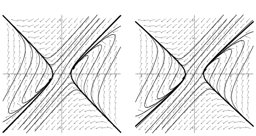
FIG. 1.: The phase diagram ($b_{0}>0$) with $\gamma=1$ and $\gamma=1.25$.

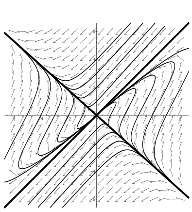
FIG. 2.: The phase diagram for $b_{0}=0$ with $a=0$.

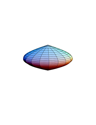
FIG. 3.: A schematic representation of the $(r,\theta)$ spatial section for a string/anti-string pair.

REFERENCES

• [1]
• [2] A.Vilenkin and E.P.S.Shellard, Cosmic strings and other Topological Defects (Cambridge Univ. Press, Cambridge, 1994). R.H.Brandenberger, Modern Cosmology and Structure Formation astro-ph/9411049. M.Hindmarsh and T.W.B.Kibble, Rep. Prog. Phys. 58 477 (1995). [hep-ph/9411342]
• [3] T.Vachaspati and A.Achucarro, Phys. Rev. D44 3067 (1991).
• [4] A.Vilenkin, Phys. Rev. D23 852 (1981). J.R.Gott III, Ap. J. 288 422 (1985). W.Hiscock, Phys. Rev. D31 3288 (1985). B.Linet, Gen. Rel. Grav. 17 1109 (1985). D.Garfinkle, Phys. Rev. D32 1323 (1985). R.Gregory, Phys. Rev. Lett. 59 740 (1987).
• [5] M.Ortiz, Phys. Rev. D45 2586 (1992). K.Lee, V.P.Nair, and E.J.Weinberg, Phys. Rev. D45 2751 (1992). [hep-th/9112008]
• [6] A.G.Cohen and D.B.Kaplan, Phys. Lett. 215B 67 (1988). D.Harari and P.Sikivie, Phys. Rev. D37 3438 (1988). R.Gregory, Phys. Lett. 215B 663 (1988). G.Gibbons, M.Ortiz and F.Ruiz, Phys. Rev. D39 1546 (1989).
• [7] R.Gregory, Phys. Rev. D54 4955 (1996). [gr-qc/9606002]
• [8] M.Barriola and A.Vilenkin, Phys. Rev. Lett. 63 341 (1989).
• [9] D.Harari and C.Lousto, Phys. Rev. D42 2626 (1990).
• [10] A.Wang and J.A.C.Nogales, Phys. Rev. D56 6217 (1997). [gr-qc/9706072]
• [11] J.Scherk and J.Schwarz, Nucl. Phys. B81 223 (1974). Phys. Lett. 52B 347 (1974). E.Fradkin and A.Tseytlin, Phys. Lett. 158B 316 (1985). C.Callan, D.Friedan, E.Martinec and M.Perry, Nucl. Phys. B262 593 (1985). C.Lovelace, Nucl. Phys. B273 413 (1985).
• [12] P.Jordan, Zeit. Phys. 157 112 (1959). C.Brans and R.H.Dicke, Phys. Rev. 124 925 (1961).
• [13] C.Gundlach & M.Ortiz, Phys. Rev. D42 2521 (1990). L.O.Pimental & A.N.Morales, Rev. Mex. Fis. 36 S199 (1990). M.E.X.Guimaraes, Class. Quantum Grav. 14 435 (1997).
• [14] A.Barros and C.Romero, Phys. Rev. D56 6688 (1997). [gr-qc/9707040] A.Banerjee, A.Beesham, S.Chatterjee, A.A.Sen, gr-qc/9710002, to appear in Classical and Quantum Gravity.
• [15] R.D.Reasenberg et.al., Ap. J. 234 L219 (1979).
• [16] A.Linde and A.Riotto, Phys. Rev. D56 1841 (1997). [hep-ph/9703209] A.Riotto, hep-ph/9710329.
• [17] A.A.Sen, N.Banerjee and A.Banerjee, Phys. Rev. D56 3706 (1997).
• [18] A.Vilenkin, Phys. Lett. 133B 177 (1983). J.Ipser and P.Sikivie, Phys. Rev. D30 712 (1984).
• [19] R.Gregory and C.Santos, Phys. Rev. D56 1194 (1997). [gr-qc/9701014]
• [20] O.Dando and R.Gregory, gr-qc/9709029, to appear in Classical and Quantum Gravity.
• [21] M.Hindmarsh and A.Wray, Mod. Phys. Lett. A 6 1249 (1991). S.Larson and W.Hiscock, Phys. Rev. D56 3242 (1997). [gr-qc/9704028]
• [22] T.Damour and A.Vilenkin, Phys. Rev. Lett. 78 2288 (1997). [gr-qc/9610005]
• [23] A.D.Linde Phys. Lett. 327B 208 (1994). [astro-ph/9402031] A.Vilenkin, Phys. Rev. Lett. 72 3137 (1994). [hep-th/9402085]
• [24] B.Boisseau and B.Linet, gr-qc/9802007
Refer to caption