Cauchy-perturbative matching and outer boundary conditions I: Methods and tests

Abstract

We present a new method of extracting gravitational radiation from three-dimensional numerical relativity codes and providing outer boundary conditions. Our approach matches the solution of a Cauchy evolution of Einstein’s equations to a set of one-dimensional linear wave equations on a curved background. We illustrate the mathematical properties of our approach and discuss a numerical module we have constructed for this purpose. This module implements the perturbative matching approach in connection with a generic three-dimensional numerical relativity simulation. Tests of its accuracy and second-order convergence are presented with analytic linear wave data.

I Introduction

An important goal of numerical relativity is to compute the gravitational waveforms generated by systems of compact astrophysical objects such as binary black holes or binary neutron stars. With the prospect that gravitational wave detectors such as LIGO, VIRGO and GEO will be on-line in the next few years, it is crucial to study numerical relativistic simulations of events which might be observable by these detectors. Such calculations are important not only because they could provide signal templates which would considerably increase the probability of detection, but also because the comparison of such templates with the observations may provide essential astrophysical information on the nature of the emitting sources. The purpose of the Binary Black Hole “Grand Challenge” Alliance [1], a multi-institutional collaboration in the United States, is to study the inspiral coalescence of the most significant source of signals for the interferometric gravity wave detectors: a binary black hole system.

Central to the goal of determining waveforms generated by astrophysical systems is the need for accurate techniques which compute asymptotic waveforms from numerical relativity simulations on three-dimensional (3D) spacelike hypersurfaces with finite extents. In general, the computational domain cannot be extended to the distant wave zone [2], where the geometric optics approximation is valid. Indeed, computational resource limitations require that the outer boundary of such simulations lies rather close to the highly dynamical and strong field region, where backscatter of waves off curvature can be significant. As a result, it is imperative to develop techniques which can “extract” the gravitational waves generated by the simulation and evolve them out to the distant wave zone where they assume their asymptotic form.

While the problem of radiation extraction is important for computing observable waveforms from numerical simulations, careful implementation of outer boundary conditions is also crucial for maintaining the integrity of the simulations themselves, as poorly implemented boundary conditions are a likely source of numerical instabilities. These outer boundary conditions are also decisive in framing the desired physical context for the simulation, e.g., an isolated source in an asymptotically flat spacetime. For typical applications, we can summarize the requirements of a radiation-extraction/outer-boundary module as: (a) supporting stable evolution of Einstein’s equations, (b) minimizing spurious (numerical) reflection of radiation at the boundary, (c) providing accurate and numerically convergent approximations to the gravitational waveforms that would be observed in the wave zone surrounding an isolated source, (d) incorporating effects of radiation reflection off background curvature outside the numerical boundary when appropriate (for example when the outer boundary is in a strong field region).

In this paper we present a new method for extracting gravitational waveforms from a 3D numerical relativity code while simultaneously imposing outer boundary conditions. Our approach is motivated by earlier investigations of gauge-invariant extraction techniques [3], but promises to be more generally applicable in cases where the background curvature is significant near the outer boundary of the computational 3D grid. Our method matches a full 3D Cauchy solution of Einstein’s equations on spacelike hypersurfaces with a perturbative one-dimensional (1D) solution in a region where the waveforms can be treated as linear perturbations on a spherically symmetric curved background .

The plan of this paper is as follows: in Section II, we describe the mathematical basis of our method and derive the linearized radial wave equations which account for the evolution of the gravitational waves in the perturbative region of the spacetime. In Section III, we discuss the strategies for the numerical solution of the above equations and present a numerical code we have constructed which represents a general module implementing our extraction/outer boundary method in conjunction with a 3D numerical relativity simulation. In this paper we focus on tests of the outer boundary module as a self-contained unit using analytic solutions. In companion papers we focus on tests of the module in the practical context of a typical application. In [5], we have presented tests of this outer boundary module in conjunction with the 3D “interior code” of the Alliance which evolves Einstein equations in the standard “$3+1$” form (as presented in [6]). A more thorough discussion of these results is forthcoming [7].

II The Cauchy-perturbative matching method

Einstein’s equations are highly nonlinear and when spacetime is characterized by rapidly varying strong fields, the full 3D nonlinear equations must be used. Outside of an isolated region of this kind, however, a perturbative approximation, in which gravitational data are treated as linear perturbations of an exact solution to Einstein’s equations, may be valid. In this perturbative region a linearized approximation to Einstein’s equations could then exploited to simplify the evolution of gravitational data.

The idea behind a Cauchy-perturbative matching approach is to supplement the computationally expensive evolution of the full Einstein equations with the comparatively simpler evolution of the linearized equations in a perturbative region. Figure 1 provides a schematic picture of the Cauchy-perturbative matching approach. The square region covered by the grid represents the 3D computational domain N (one dimension is suppressed) on which Cauchy evolution of the full Einstein equations is computed. The dark central area in N includes the strong field highly dynamical region, where the nonlinear Einstein equations must be solved. The medium and light shaded annular area, ${\cal P}$, represents the perturbative region. Anywhere in the (medium shaded) intersection of N and ${\cal P}$, we can place an extraction 2-sphere E, of radius $r_{{}_{E}}$, where the gravitational field information is read out. This information is then evolved (by means of the linearized Einstein equations) in ${\cal P}$, which ranges from E out to a large distance (shown as a dotted circle) where the asymptotic waveforms can be identified. Outer boundary data for N can be constructed from perturbative data in the intersection of N and ${\cal P}$.

Previous investigations [3] achieved the desired perturbative simplification by matching the nonlinear solution onto analytic solutions of Einstein’s equations linearized on a Minkowski background. Further simplification was achieved by decomposing perturbative data in a multipole expansion. We extend this approach to cases where curvature is significant by choosing as our approximation a linearization of Einstein’s equations on a Schwarzschild background. In principal one could generalize further to a Kerr background, and this will be the subject of future work. We also decompose perturbative data on this background with a multipole expansion, reducing the 3D linearized equations to a set of 1D equations for each multipole mode. This reduction allows us to evolve data everywhere in ${\cal P}$ on a one-dimensional grid, L. It is important to note that all of the 3-dimensional tensor data in ${\cal P}$ can be reconstructed from the multipole amplitudes on L. Our method, therefore, is to match a computationally expensive evolution of the full Einstein equations onto a considerably less expensive evolution on a 1D grid in a region where background curvature is still significant.

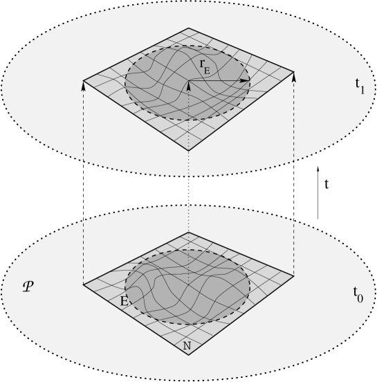
FIG. 1.: Schematic of matching procedure for two successive timeslices (one dimension is suppressed). N is the 3D computational domain. The dark shaded region shows the strong field highly dynamical region in N. The medium and light shaded annular region represents the “perturbative region”, ${\cal P}$, where the linearized equations are evolved on a 1D grid L (not shown).

A Hyperbolic formulation

Rather than characterize radiation asymptotically in terms of certain variables constructed from the metric [3], we use a new approach which characterizes radiation in terms of the extrinsic curvature. This is made possible by a recently developed spatially gauge-covariant hyperbolic formulation of general relativity. This system is constructed from first derivatives of the spacetime Ricci tensor [8, 9, 10] and may therefore appropriately be called the “Einstein–Ricci” system.

The Einstein–Ricci equations are obtained from the “$3+1$” form of the metric,

$$ds^{2}=-N^{2}dt^{2}+g_{ij}(dx^{i}+\beta^{i}dt)(dx^{j}+\beta^{j}dt)\ ,$$ (1)

where $N$ is the lapse function, $\beta^{i}$ is the shift vector, and $g_{ij}$ is the spatial metric in the slice $\Sigma$. An appropriate time derivative operator that evolves spatial quantities along the normal to the slice $\Sigma$ is

$$\hat{\partial}_{0}=\partial_{t}-{\cal L}_{\beta}\ ,$$ (2)

where ${\cal L}_{\beta}$ is the Lie derivative along the shift vector in $\Sigma$.

The extrinsic curvature $K_{ij}$ of $\Sigma$ can be defined by

$$\hat{\partial}_{0}g_{ij}=-2NK_{ij}\ ,$$ (3)

which serves also as the evolution equation for the spatial metric. By working out the expression $\Omega_{ij}\equiv\hat{\partial}_{0}R_{ij}-2\overline{\nabla}_{(i}R_{j)0}$ in $3+1$ form, where $R_{ij}$ and $R_{j0}$ are components of the spacetime Ricci tensor and $\overline{\nabla}_{i}$ denotes the spatial covariant derivative, we find a wave-like equation which governs the evolution of $K_{ij}$:

$$-N\hat{\mbox{\kern 0.0pt\lower 1.29167pt\hbox{$\Box$}}}K_{ij}=J_{ij}+S_{ij}-\Omega_{ij}\ ,$$ (4)

where the physical wave operator for arbitrary shift is $\hat{\mbox{\kern 0.0pt\lower 1.29167pt\hbox{$\Box$}}}\equiv-N^{-1}\hat{\partial}_{0}N^{-1}\hat{\partial}_{0}+\overline{\nabla}_{k}\overline{\nabla}^{k}$. Equation (4) is an identity until we substitute the Einstein equations $R_{\alpha\beta}=8\pi(T_{\alpha\beta}-\frac{1}{2}T^{\lambda}_{\lambda}g_{\alpha\beta})$ into $\Omega_{ij}$ ( $G=c=1$ ).

The detailed form of the right hand side of (4) can be found in [9, 10]; the present conventions are those in [10]. Here we simply point out that $\Omega_{ij}$ has become a matter source that is zero here, $J_{ij}$ is the nonlinear self-interaction term in $3+1$ form, and $S_{ij}$ is a slicing-dependent term that must involve fewer than second derivatives of $K_{ij}$ to render (4) a true (hyperbolic) wave equation. A simple way to satisfy the restriction on $S_{ij}$ is to invoke the harmonic slicing condition

$$\hat{\partial}_{0}N+N^{2}H=0,$$ (5)

where $H$ is the trace of $K_{ij}$, and from which follows $S_{ij}=0$.

For appropriate choice of initial data [9, 10], equations (3), (4), and (5) represent the dynamical part of Einstein’s equations. Combining them we obtain a quasi-diagonal hyperbolic equation for $g_{ij}$, with principal (highest-order) part $\hat{\mbox{\kern 0.0pt\lower 1.29167pt\hbox{$\Box$}}}\hat{\partial}_{0}$. Hence (3), (4), and (5) may be said to give the “third-order” form of the Einstein–Ricci system.

We note that the third-order Einstein–Ricci system can also be cast into a first-order symmetric hyperbolic form [9, 10, 11].  It also possesses a higher order form (the “fourth-order Einstein–Ricci system”), essentially a wave equation for $(\hat{\partial}_{0}K_{ij})$, obtained from $\hat{\partial}_{0}\Omega_{ij}+\overline{\nabla}_{i}\overline{\nabla}_{j}R_{00}$ [11, 12, 13]. This system has a well-posed Cauchy problem and complete freedom in choosing both $\beta^{i}$ and $N$: it has no analog of a slicing term like $S_{ij}$. This fourth-order form is used to develop fully gauge-invariant perturbation theory in [14].

B Perturbative Expansion

The first step in obtaining radial wave equations is to linearize the hyperbolic Einstein-Ricci equations around a static Schwarzschild background. We separate the gravitational quantities of interest into background (denoted by a tilde) and perturbed parts: the 3-metric $g_{ij}=\widetilde{g}_{ij}+h_{ij}$, the extrinsic curvature $K_{ij}=\widetilde{K}_{ij}+\kappa_{ij}$, the lapse $N=\widetilde{N}+\alpha$, and the shift vector $\beta^{i}=\widetilde{\beta}^{i}+v^{i}$. In Schwarzschild coordinates $(t,r,\theta,\phi)$, the background quantities are given by

$$\widetilde{N} = \left(1-\frac{2M}{r}\right)^{1/2}\ ,$$ (7)

$$\widetilde{g}_{ij}dx^{i}dx^{j} = \widetilde{N}^{-2}dr^{2}+r^{2}(d\theta^{2}+\sin^{2}\theta d\phi^{2})\ ,$$ (8)

$$\widetilde{\beta}^{i} = 0\ ,$$ (9)

$$\widetilde{K}_{ij} = 0\ ,$$ (10)

while the perturbed quantities have arbitrary angular dependence. The background quantities satisfy the dynamical equations $\partial_{t}\widetilde{g}_{ij}=0$, $\partial_{t}\widetilde{N}=0$, and thus remain constant for all time. The perturbed quantities, on the other hand, obey the following evolution equations

$$\partial_{t}h_{ij} = -2\widetilde{N}\kappa_{ij}+2\widetilde{\nabla}_{(i}v_{j)}\ ,$$ (12)

$$\partial_{t}\alpha = v^{i}\widetilde{\nabla}_{i}\widetilde{N}-\widetilde{N}^{2}\kappa\ ,$$ (13)

$$\widetilde{N}^{-1}\partial_{t}^{2}\kappa_{ij}-\widetilde{N}\widetilde{\nabla}^{k}\widetilde{\nabla}_{k}\kappa_{ij}= - 4\widetilde{\nabla}_{(i}\kappa^{k}_{\ j)}\widetilde{\nabla}_{k}\widetilde{N}+\widetilde{N}^{-1}\kappa_{ij}\widetilde{\nabla}^{k}\widetilde{N}\widetilde{\nabla}_{k}\widetilde{N}+3\widetilde{\nabla}^{k}\widetilde{N}\widetilde{\nabla}_{k}\kappa_{ij}$$ (14)

$$+ \kappa_{ij}\widetilde{\nabla}^{k}\widetilde{\nabla}_{k}\widetilde{N}-2\kappa^{k}_{\;(i}\widetilde{\nabla}_{j)}\widetilde{\nabla}_{k}\widetilde{N}-2\widetilde{N}^{-1}\kappa^{k}_{\;(i}\widetilde{\nabla}_{j)}\widetilde{N}\widetilde{\nabla}_{k}\widetilde{N}+2\kappa\widetilde{\nabla}_{i}\widetilde{\nabla}_{j}\widetilde{N}$$ (15)

$$+ 4\partial_{(i}\kappa\partial_{j)}\widetilde{N}+2\widetilde{N}^{-1}\kappa\widetilde{\nabla}_{i}\widetilde{N}\widetilde{\nabla}_{j}\widetilde{N}-2\widetilde{N}\widetilde{R}_{k(i}\kappa^{k}_{\ j)}-2\widetilde{N}\widetilde{R}_{kijm}\kappa^{km}\ ,$$ (16)

where $\kappa\equiv\kappa^{i}_{\ i}$ and the tilde denotes a spatial quantity defined in terms of the background metric, $\widetilde{g}_{ij}$. Note that the wave equation for $\kappa_{ij}$ involves only the background lapse and curvature.

C Angular decomposition

We can further simplify the evolution equation (16) by separating out the angular dependence, thus reducing it to a set of 1D equations. We accomplish this by expanding the extrinsic curvature in Regge–Wheeler tensor spherical harmonics [16] and substituting this expansion into (16). Using the notation of Moncrief [15] we express the expansion as

$$\kappa_{ij}=a_{\times}(t,r)(\hat{e}_{1})_{ij}+rb_{\times}(t,r)(\hat{e}_{2})_{ij}+\widetilde{N}^{-2}a_{+}(t,r)(\hat{f}_{2})_{ij}+rb_{+}(t,r)(\hat{f}_{1})_{ij}+\hskip 28.45274pt$$ (17)

$$r^{2}c_{+}(t,r)(\hat{f}_{3})_{ij} + r^{2}d_{+}(t,r)(\hat{f}_{4})_{ij}\ ,$$ (18)

where $(\hat{e}_{1})_{ij},\cdots,(\hat{f}_{4})_{ij}$ are the Regge–Wheeler harmonics, which are functions of $(\theta,\phi)$ and have suppressed angular indices $(\ell,m)$ for each mode. The odd-parity multipoles ($a_{\times}$ and $b_{\times}$) and the even-parity multipoles ($a_{+}$, $b_{+}$, $c_{+}$, and $d_{+}$) also have suppressed indices for each angular mode and there is an implicit sum over all modes in (18). The six multipole amplitudes correspond to the six components of $\kappa_{ij}$. However, using the linearized momentum constraints

$$\widetilde{\nabla}_{j}(\kappa^{j}_{\ i}-\delta^{j}_{\ i}\kappa)=0\ ,$$ (19)

we reduce the number of independent components of $\kappa_{ij}$ to three. An important relation is also obtained through the wave equation for $\kappa$, whose multipole expansion is simply given by $\kappa=h(t,r)Y_{{}_{\ell m}}$ where $Y_{{}_{\ell m}}(\theta,\phi)$ is the standard scalar spherical harmonic and again there is an implicit sum over suppressed indices $(\ell,m)$. Using this expansion, in conjunction with the momentum constraints (19), we derive a set of radial constraint equations which relate the dependent amplitudes $(b_{\times})_{{}_{\ell m}}$, $(b_{+})_{{}_{\ell m}}$, $(c_{+})_{{}_{\ell m}}$ and $(d_{+})_{{}_{\ell m}}$ to the three independent amplitudes $(a_{\times})_{{}_{\ell m}}$, $(a_{+})_{{}_{\ell m}}$, $(h)_{{}_{\ell m}}$:

$$(b_{\times})_{{}_{\ell m}} = -\frac{1}{(\ell+2)(\ell-1)}[(1+3\widetilde{N}^{2})+2\widetilde{N}^{2}r\;\partial_{r}]\;(a_{\times})_{{}_{\ell m}}\ ,$$ (21)

$$(b_{+})_{{}_{\ell m}} = \frac{1}{\ell(\ell+1)}[(3+r\partial_{r})\;(a_{+})_{{}_{\ell m}}-(1+r\partial_{r})\;(h)_{{}_{\ell m}}]\ ,$$ (22)

$$(c_{+})_{{}_{\ell m}} = \frac{1}{2(\ell+2)(\ell-1)}\{2(1-\ell-\ell^{2})\;(a_{+})_{{}_{\ell m}}-2\;(h)_{{}_{\ell m}}+\ell(\ell+1)[(1+5\widetilde{N}^{2})+2\widetilde{N}^{2}r\;\partial_{r}]\;(b_{+})_{{}_{\ell m}}\}\ ,$$ (23)

$$(d_{+})_{{}_{\ell m}} = \frac{1}{\ell(\ell+1)}[(a_{+})_{{}_{\ell m}}+2(c_{+})_{{}_{\ell m}}-(h)_{{}_{\ell m}}]\ ,$$ (24)

for each $(\ell,m)$ mode.

Substituting (18) into (16) and using the constraint equations (II C), we obtain a set of linearized radial wave equations for each independent amplitude. For each $(\ell,m)$ mode we have one odd-parity equation

$$\Biggl{\{}\partial^{2}_{t}-\widetilde{N}^{4}\partial^{2}_{r}-\frac{2}{r}\widetilde{N}^{2}\partial_{r}-\frac{2M}{r^{3}}\left(1-\frac{3M}{2r}\right)+\widetilde{N}^{2}\left[\frac{\ell(\ell+1)}{r^{2}}-\frac{6M}{r^{3}}\right]\Biggr{\}}(a_{\times})_{{}_{\ell m}}=0\ ,$$ (25)

and two coupled even-parity equations,

$$\hskip 0.0pt\Biggl{[}\partial^{2}_{t}-\widetilde{N}^{4}\partial^{2}_{r}-\frac{6}{r}\widetilde{N}^{4}\partial_{r}+\widetilde{N}^{2}\frac{\ell(\ell+1)}{r^{2}}-\frac{6}{r^{2}}+\frac{14M}{r^{3}}-\frac{3M^{2}}{r^{4}}\Biggr{]}(a_{+})_{{}_{\ell m}}+\hskip 170.71652pt$$ (26)

$$\Biggl{[}\frac{4}{r}\widetilde{N}^{2}\left(1-\frac{3M}{r}\right)\partial_{r}+\frac{2}{r^{2}}\left(1-\frac{M}{r}-\frac{3M^{2}}{r^{2}}\right)\Biggr{]}(h)_{{}_{\ell m}}=0\ ,$$ (27)

$$\Biggl{[}\partial^{2}_{t}-\widetilde{N}^{4}\partial^{2}_{r}-\frac{2}{r}\widetilde{N}^{2}\partial_{r}+\widetilde{N}^{2}\frac{\ell(\ell+1)}{r^{2}}+\frac{2M}{r^{3}}-\frac{7M^{2}}{r^{4}}\Biggr{]}(h)_{{}_{\ell m}}-\frac{2M}{r^{3}}\left(3-\frac{7M}{r}\right)(a_{+})_{{}_{\ell m}}=0\ .$$ (28)

These equations are related to the standard Regge–Wheeler and Zerilli equations [16, 17], which can be derived in a more complete analysis of gauge-invariant hyperbolic formulations [14].

The radial wave equations (25)–(28) for each $(\ell,m)$ mode of the independent multipole amplitudes $(a_{\times})_{{}_{\ell m}}$, $(a_{+})_{{}_{\ell m}}$, $(h)_{{}_{\ell m}}$ form the basis for our approach. In the perturbative region, they replace the nonlinear Einstein equations and determine the evolution of $K_{ij}$. They can be used to evolve, with minimal computational cost, gravitational wave data to arbitrarily large distances from the highly dynamical strong field region. The evolution equations for $h_{ij}$ (12) and $\alpha$ (13) can also be integrated using the data for $K_{ij}$ computed in this region. Note that because $h_{ij}$ and $\alpha$ evolve along the coordinate time axis, these equations need only be integrated in the region in which their values are desired, not over the whole region L (these quantities have characteristic speed zero).

III Numerical Implementation

This section is a general guide for the numerical implementation of the Cauchy-perturbative matching method for radiation extraction and outer boundary conditions described so far.

Consider a 3D numerical relativity code which solves the Cauchy problem of Einstein’s equations in either the standard ADM form [18] or in the hyperbolic form [19]. During each timestep the procedure followed by our module for extracting radiation and imposing outer boundary conditions can be summarized in three successive steps: (1) extraction of the independent multipole amplitudes on E, (2) evolution of the radial wave equations (25)–(28) on L out to the distant wave zone, (3) reconstruction of $K_{ij}$ and $\partial_{t}K_{ij}$ at specified gridpoints at the outer boundary of N. We now discuss in detail each of these steps:

  

(1)   Extraction

As mentioned in Sect. II, the extraction 2-sphere E acts as the joining surface between the evolution of the highly dynamical, strong field region (dark shaded area of Fig. 1) and the perturbative regions (light shaded areas). At each timestep, $K_{ij}$ and $\partial_{t}K_{ij}$ are computed on N as a solution to Einstein’s equations. In the test cases presented here, N uses topologically Cartesian coordinates, although there are no restrictions on the choice of the coordinate system. The Cartesian components of these tensors are then transformed into their equivalents in a spherical coordinate basis and their traces are computed using the inverse background metric, i.e. $H=\widetilde{g}^{ij}K_{ij}$, $\partial_{t}H=\widetilde{g}^{ij}\partial_{t}K_{ij}$. From the spherical components of $K_{ij}$ and $\partial_{t}K_{ij}$, the independent multipole amplitudes for each $(\ell,m)$ mode are then derived by an integration over the 2-sphere:

$$(a_{\times})_{{}_{\ell m}} = \frac{1}{\ell(\ell+1)}\int\;\frac{1}{\sin\theta}\left[K_{r\phi}\;\partial_{\theta}-K_{r\theta}\;\partial_{\phi}\right]\;{Y^{*}_{{}_{\ell m}}}\;d\Omega\ ,$$ (30)

$$(a_{+})_{{}_{\ell m}} = \int\;\widetilde{N}^{2}\;K_{rr}\;Y^{*}_{\ell m}\;d\Omega\ ,$$ (31)

$$(h)_{{}_{\ell m}} = \int\;H\;Y^{*}_{\ell m}d\Omega\ .$$ (32)

Their time derivatives are computed similarly. Rather than performing the integrations (30)–(32) using spherical polar coordinates, it is useful to cover E with two stereographic coordinate “patches”. These are uniformly spaced two-dimensional (2D) grids onto which the values of $K_{ij}$ and $\partial_{t}K_{ij}$ are interpolated using either a three-linear or a three-cubic polynomial interpolation scheme. Each point on the 2-sphere, denoted by spherical coordinate values $(\theta,\phi)$, corresponds to a point $(q,p)$ on a stereographic grid whose coordinates can be combined into a single complex number $\zeta$:

$$\zeta_{{}_{N}} \equiv q_{{}_{N}}+ip_{{}_{N}}=\tan\left(\frac{\theta}{2}\right){\rm e}^{i\phi}\ ,$$ (34)

$$\zeta_{{}_{S}} \equiv q_{{}_{S}}+ip_{{}_{S}}=\frac{1}{\zeta_{{}_{N}}}\ ,$$ (35)

where $N$ and $S$ denote the northern ($0\leq\theta\leq\pi/2$) and southern ($\pi/2\leq\theta\leq\pi$) hemispheres, respectively. As a result of this transformation, the integrals over the 2-sphere in ( ‣ III) are computed over the stereographic patches, which naturally avoid polar singularities (see [20] for a complete discussion of the properties and advantages of the stereographic coordinates). In our tests, the integrals over each patch are computed using a second-order stereographic quadrature routine developed within the Alliance [20].

  

(2)   Evolution

Once the multipole amplitudes, $(a_{\times})_{{}_{\ell m}}$, $(a_{+})_{{}_{\ell m}}$, $(h)_{{}_{\ell m}}$ and their time derivatives are computed on E in the timeslice $t=t_{0}$, they are imposed as inner boundary conditions on the 1D grid. Using a second-order integration scheme (we have tested both Leapfrog and Lax-Wendroff [21]), our module then evolves the radial wave equations (25)–(28) for each $(\ell,m)$ mode forward to the next timeslice at $t=t_{1}$. The outer boundary of the 1D grid is always placed at a distance large enough that background field and near-zone effects are unimportant, and a radial Sommerfeld condition for the wave equations (25)–(28) can be imposed there. Of course, the initial data on L must be consistent with the initial data on N. This can either be imposed analytically or determined by applying the aforementioned extraction procedure to the initial data set at each gridpoint of L in the region of overlap with N. In the latter case, initial data outside the overlap region can be set by considering the asymptotic fall-off of each variable. It should be noted that in the Cauchy-characteristic matching approach initial data also must be set in the characteristic hypersurfaces and, for realistic sources like binary black holes, will necessarily be approximate.

  

(3)   Reconstruction and Matching

From the perturbative data evolved to time $t_{1}$, outer boundary values for N can now be computed. The procedure for doing this differs depending on whether a hyperbolic or an ADM formulation of Einstein’s equations is used by the 3D “interior code”. For a hyperbolic code (cf. [19]), it is necessary to provide boundary data for $K_{ij}$ and $\partial_{t}K_{ij}$. For an ADM code (cf. [18]), on the other hand, outer boundary data only for $K_{ij}$ are necessary, since the interior code can calculate $g_{ij}$ at the outer boundary by integrating in time the boundary values for $K_{ij}$. In either case, if outer boundary values for the lapse $N$ are needed [e.g. for integrating harmonic slicing condition (5)], these can be computed by the perturbative module or by integration of $H$ at the boundary.

In order to compute $K_{ij}$ at an outer boundary point of N (or any other point in the overlap between N and ${\cal P}$ [7]), it is necessary to reconstruct $K_{ij}$ from the multipole amplitudes and tensor spherical harmonics. The Schwarzschild coordinate values $(r,\theta,\phi)$ of the relevant gridpoint are first determined. Next, $(a_{\times})_{{}_{\ell m}}$, $(a_{+})_{{}_{\ell m}}$, and $(h_{{}_{\ell m}})$ for each $(\ell,m)$ mode are interpolated to the radial coordinate value of that point. The dependent multipole amplitudes $(b_{\times})_{{}_{\ell m}}$, $(b_{+})_{{}_{\ell m}}$, $(c_{+})_{{}_{\ell m}}$, and $(d_{+})_{{}_{\ell m}}$ are then computed using the constraint equations (II C). Finally, the Regge–Wheeler tensor spherical harmonics $(\hat{e}_{1})_{ij}$–$(\hat{f}_{4})_{ij}$ are computed for the angular coordinates $(\theta,\phi)$ for each $(\ell,m)$ mode and the sum in equation (18) is performed. This leads to the reconstructed component of $\kappa_{ij}$ (and therefore $K_{ij}$); a completely analogous algorithm is used to reconstruct $\partial_{t}K_{ij}$.

It is important to emphasize that this procedure allows one to compute $K_{ij}$ at any point of N which is covered by the perturbative region. As a result, the numerical module can reconstruct the values of $K_{ij}$ and $\partial_{t}K_{ij}$ on a 2-surface of arbitrary shape, or any collection of points outside of E.

Numerical implementation of this method is rather straightforward. Very few modifications to a standard 3D numerical relativity code are necessary in order to allow for the simultaneous evolution of the highly dynamical region and of the perturbative one. Because of the use of numerically inexpensive integration of 1D wave equations, implementation of this module provides gravitational wave extraction and stable outer boundary conditions with only minimal additional computational cost.

Finally, it should be noted that, in practice, we may not know a priori if the Schwarzschild-perturbative approximation is valid near the outer boundary of a given numerical relativity simulation. Through experimentation, however, it is possible to test the validity of the approximation. This can be done, for instance, by extracting data at different radii and comparing the waveforms computed at the outer sphere with those evolved from the inner sphere. This makes it possible to determine if the neglected terms in the approximation have a significant effect. At any point in the overlap region between N and ${\cal P}$, it is possible to reconstruct gravitational wave data and compare these values with those computed by the full nonlinear evolution.

IV Numerical tests

In order to establish the accuracy and convergence properties of our code we have studied the propagation of linear waves on a Minkowski background ($M=0$) . This is a natural first test since we can compare each stage of the numerical procedure described in Section III against a known analytic solution [22, 23].

In these tests we assign analytic values to each gridpoint of N at every time step. This allows us to study the accuracy and convergence properties of the module independently of any errors which may develop in a 3D numerical evolution of linear waves. Elsewhere [7], we will present results of tests of this module running with a full 3D evolution code (i.e. the interior code of the Alliance [18]), with emphasis on the issues of stability of the outer boundary and accuracy of extracted waveforms.

We have considered analytic data for $\ell=2$, $m=0$ even-parity linear waves, initially modulated by a Gaussian envelope with amplitude $A=10^{-6}$ and width parameter $b=1$. These waves are time-symmetric at $t=0$ and thus have ingoing and outgoing parts. The 3D grid is vertex-centered with extents $(x,y,z)\in[-4,4]$ and resolutions ranging from $(17)^{3}$ to $(129)^{3}$ points [corresponding to $(16)^{3}$ and $(128)^{3}$ zones, respectively]. The resolution of the stereographic coordinate patches corresponds to the resolution of N and therefore ranges from $(16)^{2}$ to $(128)^{2}$ zones on each hemisphere. For the specific tests presented here, E is located at a radius $r_{{}_{E}}=3$ and similar results have been obtained also for $r_{{}_{E}}=0.5,1.0,1.5,2,2.5,3.5$. In fact, on a flat background spacetime and for weak waves on Schwarzschild-like backgrounds, the perturbative approximation is valid throughout the 3D domain and the position of E is thus arbitrary.

Since these waves are traceless and even-parity, with pure $\ell=2$, $m=0$ angular dependence, the only non-zero independent multipole amplitude we expect to find at E is $(a_{+})_{{}_{20}}$. Diagram (a) of Fig. 2 shows plots of $(a_{+})_{{}_{20}}$ extracted at $r_{{}_{E}}=3$ as a function of $t-r$ for various resolutions of N. The amplitude is scaled by $r^{3}$ to compensate for the radial fall-off.

The curves in diagram (a) clearly show that the extracted waveform approaches the analytic value (denoted by a solid line) as the resolution is increased. However, in order to establish the exact rate at which the computed solution approaches the analytic one, we have also performed convergence tests. These tests are designed to check that no coding error has been made and that the numerical scheme employed in the solution is providing results at the expected accuracy. While there are a number of different ways to perform these tests, we have exploited the knowledge of an analytic solution and computed the residuals $R$ between the computed solution ${\mathcal{F}}_{c}$ and the analytic one ${\mathcal{F}}_{a}$ as a function of the resolution (or, equivalently, of the number of gridpoints). For a second-order accurate numerical scheme (as the one used here) on a uniform cubical grid, we expect the residuals to follow the simple law

$$R(N^{3})={\mathcal{F}}_{c}-{\mathcal{F}}_{a}=O(h^{2})\ ,$$ (36)

where $O(h^{2})$ contains the second and higher order error terms and $h=L/(N-1)$ is the grid resolution, with $L$ being the spatial dimension of the grid. If the numerical computation is second-order accurate and a number of simulations with different grid resolutions, each differing by a factor 2, are performed, we should expect the residual to fall quadratically to zero. Diagram (b) of Fig. 2 shows this is indeed the case; there, we have multiplied the residuals obtained with different resolutions by the coefficients that make the leading order error terms comparable. The good overlapping of the different curves is an indication that a second-order convergence has been achieved.

FIG. 2.: (a) Timeseries of the multipole amplitude $(a_{+})_{{}_{20}}$ extracted at a 2-sphere of radius $r_{{}_{E}}=3$ for various grid resolutions. The amplitude is scaled by $r^{3}$ to compensate for the radial fall-off. (b) Residuals of the leading order error term for different grid resolutions differing by a factor of 2. The residuals are multiplied by 4, 16, and 64 in order to make the errors comparable. If no higher-order terms were present, all of the curves would coincide.

The accuracy of this extraction procedure can also be tested by examining the waveforms for the other multipole amplitudes computed which analytically vanish. Figure 3 shows plots of several even-parity (upper diagram) and odd-parity (lower diagram) amplitudes computed at the extraction 2-sphere for an resolution in N of $(65)^{3}$ points. As a result of numerical truncation error introduced in the extraction procedure, these modes are not exactly zero. However, even the largest amplitude mode is over three orders of magnitude smaller than the only analytically non-vanishing independent amplitude $(a_{+})_{{}_{20}}$. Moreover, all of these amplitudes are second-order convergent to zero as the resolution is increased. Similar considerations apply also for the $(h)_{{}_{\ell m}}$ multipole amplitudes: although the data is analytically traceless, very small $(h)_{{}_{\ell m}}$ modes are extracted at the 2-sphere. These modes, which we will not show here, are the order of round-off error (approximately $10^{-22}$ for these tests) and may be considered as effectively zero.

FIG. 3.: Timeseries of the analytically vanishing even $(a_{+})_{{}_{\ell m}}$ and odd $(a_{\times})_{{}_{\ell m}}$ parity multipole amplitudes. The extraction is made at a 2-sphere of radius $r_{{}_{E}}=3$ and N has $(65)^{3}$ points.

Next, we consider the accuracy of the evolution in the perturbative region of the extracted amplitudes. The time integration of (25)–(28) on L is performed using a Leapfrog integration scheme with a spatial resolution adjusted so that the timesteps in N and L are identical. This imposes a relation involving the gridspacing of N and the ratio of Courant factors for N and L. Such a choice ensures a correspondence between resolutions of N and ${\cal P}$ Fig. 4 shows plots of $(a_{+})_{{}_{20}}$ evolved to a radius $r=8$ from the extracted signal at $r=r_{{}_{E}}=3$. Different curves correspond to different resolutions and show the convergence to the analytic solution. The outer boundary of L is located at $r=33$, where outgoing wave Sommerfeld conditions are imposed. For radial scalar wave equations, this represents a very good approximation which has been shown to be both accurate and stable.

FIG. 4.: Timeseries of $(a_{+})_{{}_{20}}$ evolved to $r=8$ for various grid resolutions. Here also, the amplitude is scaled by $r^{3}$ to compensate for the radial fall-off.

Finally, we consider the accuracy in the reconstruction of the outer boundary data. Since we are using analytic data in N, we can only compare the outer boundary data with the analytic ones. In a forthcoming paper [7], where we will make use of a numerical solution of Einstein’s equations, we will also discuss the issues of stability related to the use of a Cauchy-perturbative matching method. For conciseness we consider here reconstructed outer boundary data only for $K_{ij}$; the reconstruction of $\partial_{t}K_{ij}$ follows analogously. Diagram (a) of Fig. 5 shows the timeseries of the reconstructed value of $K_{zz}$ computed at the point $(x=4,y=0,z=0)$ for various resolutions and its comparison with the analytic solution. Also in this case, diagram (b) of Fig. 5 gives proof of the second-order convergence of the numerical module even if, in this case, higher order error terms become apparent with the very coarse resolution simulations [i.e. in the case of $(17)^{3}$ gridpoints]. The small peak observed at $t-r\approx 1$ is the result of a slight difference between the analytic initial data on L and the extracted signal at $t=0$. This error rapidly disappears as the resolution is increased.

FIG. 5.: (a) Timeseries of the reconstructed values for $K_{zz}$ at the grid point $(4,0,0)$ for various grid resolutions. (b) Residuals of the leading order error term for different grid resolutions differing by a factor of 2 (cf. Fig. 2).

A more global measure of the accuracy and of the convergence properties of the boundary data is obtained by computing the $L_{2}$ norm of the error in $K_{ij}$ as measured over the whole 3D outer boundary. In Fig. 6 we plot the $L_{2}$ norms of $K_{zz}$ at successive resolutions, normalizing these differences by the factor which would make the plots overlap if the convergence to analytic data were exactly second-order. Here we again see that the desired convergence rate is achieved over the whole boundary, particularly at finer grid resolutions.

FIG. 6.: Plot of $L_{2}$ norms of $K_{zz}$ computed over the outer boundary for successive grid resolutions. The norms at different grid resolutions are scaled so that they overlap if truly second-order convergent.

V Conclusion

We have presented a method for matching gravitational data computed from a 3D Cauchy evolution of Einstein’s equations to a computationally simpler evolution of radial wave equations linearized on a Schwarzschild background. This method should be applicable to a variety of physical problems where curvature is significant throughout the computational domain, so long as the time-dependent fields can be treated as linear perturbations on a spherical background. Our approach promises to offer an accurate means of computing asymptotically gauge-invariant waveforms at large distances from the domain of the simulation and to provide stable, physically correct boundary conditions.

We have also discussed a numerical code we have developed that implements this procedure and can be used with a general numerical 3D simulation, solving Einstein’s equations in either the hyperbolic or ADM formulation. This code correctly extracts waveforms from analytic linear wave data and recomputes that data at the outer boundary of the 3D grid. A more extensive discussion of the stability properties of this approach will be discussed in a forthcoming paper [7], as well as practical issues arising from application to a real evolution code environment.

Our Cauchy-perturbative matching method can be extended to more general circumstances, e.g. perturbations on axially symmetric backgrounds or other slicings of Schwarzschild black holes. Similar analyses using other hyperbolic formulations[13, 24] may also provide important insight to the physical understanding of radiation extraction and lead to modules which work with simulations based on these formulations.

- [1] Information about the Binary Black Hole Grand Challenge Alliance, its goals and present status of research can be found at the web page: http://www.npac.syr.edu/projects/bh/.
- [2] For a full discussion on the splitting of spacetime around isolated sources, see: K. S. Thorne, Rev. Mod. Phys. 52, 299 (1980).
- [3] A. M. Abrahams and C. R. Evans, Phys. Rev. D, 37, 317 (1988); Phys. Rev. D, 42, 2585 (1990).
- [4] N. T. Bishop, R. Gómez, P. R. Holvorcem, R. A. Matzner, P. Papadopoulos and J. Winicour, Phys. Rev. Lett. 76, 4303 (1996); N. T. Bishop, R. Gómez, L. Lehner, J. Winicour, Phys. Rev. D. 54, 6153 (1996).
- [5] The Grand Challenge Alliance: A. M. Abrahams, L. Rezzolla, M. E. Rupright et al., gr-qc/9709082, Phys. Rev. Lett. In press, (1998).
- [6] J. W. York Jr. in Sources of Gravitational Radiation, edited by L. Smarr, Cambridge Univ. Press, Cambridge (1979).
- [7] L. Rezzolla, A. M. Abrahams, M. E. Rupright, In preparation.
- [8] Y. Choquet-Bruhat and T. Ruggeri, Commun. Math. Phys. 89, 269 (1983).
- [9] Y. Choquet-Bruhat and J. W. York Jr., C. R. Acad. Sci., Série I, Paris 321, 1089 (1995).
- [10] A. M. Abrahams, A. Anderson, Y. Choquet-Bruhat, and J. W. York Jr., Phys. Rev. Lett. 75, 3377 (1995).
- [11] A. M. Abrahams, A. Anderson, Y. Choquet-Bruhat, and J. W. York Jr., Class. Quantum Grav. 14 A9 (1997).
- [12] A. M. Abrahams, A. Anderson, Y. Choquet-Bruhat, and J. W. York Jr., C. R. Acad. Sci., Série IIb, Paris 323 835 (1996).
- [13] Y. Choquet-Bruhat and J. W. York Jr., Banach Center Publications, 41, Part 1, 119 (1997).
- [14] A. Anderson, A. M. Abrahams, and C. Lea, In preparation.
- [15] V. Moncrief, Ann. Phys. 88, 323 (1974).
- [16] T. Regge and J. A. Wheeler, Phys. Rev. 108, 1063 (1957).
- [17] F. Zerilli, Phys. Rev. Lett. 24 737 (1970).
- [18] The Grand Challenge Alliance: G. B. Cook, M. F. Huq, S. A. Klasky, M. A. Scheel et al., gr-qc/9711078, submitted to Phys. Rev. Lett., (1997).
- [19] M. A. Scheel et al., Phys. Rev. D 56, 6320 (1997)
- [20] R. Gómez, L. Lehner, P. Papadopoulos and J. Winicour, Class. Quantum Grav. 14, 977 (1997)
- [21] W. H. Press, B. P. Flannery, S. A. Teukoslky and W. T. Vetterling, Numerical Recipes, Cambridge University Press, Cambridge (1986).
- [22] W. L. Burke, J. Math. Phys. 12, 401 (1971).
- [23] S. A. Teukolsky, Phys. Rev. D 26, 745 (1982).
- [24] A. Anderson, Y. Choquet-Bruhat and J. W. York Jr., Topological Methods in Nonlinear Analysis, In press.