Caustics of Compensated Spherical Lens Models

Abstract

We consider compensated spherical lens models and the caustic surfaces they create in the past light cone. Examination of cusp and crossover angles associated with particular source and lens redshifts gives explicit lensing models that confirm the claims of Paper I [1], namely that area distances can differ by substantial factors from angular diameter distances even when averaged over large angular scales. ‘Shrinking’ in apparent sizes occurs, typically by a factor of 3 for a single spherical lens, on the scale of the cusp caused by the lens; summing over many lenses will still leave a residual effect.

Subject headings:
cosmology - gravitational lensing,  - observational tests

1 Introduction

This paper continues the study started in Paper I [1] of how area distances behave in universes where strong gravitational lensing takes place. That paper considered the claim [2] that although individual lensing masses alter area distances for ray bundles that pass near by them, photon conservation guarantees the same area distance-redshift relation as in exactÆ It was shown in [1] that this claimed compensation result is incorrect once one has passed caustics, which are necessarily the result of strong gravitational lensing; consequently (by continuity) the result is not true in general. Indeed it has to be wrong because area distances are determined by the gravitational field equations (essentially through the null Raychaudhuri equation) quite independently of the issue of photon conservation (which is determined by Maxwell’s equations and is valid whatever the space-time curvature). Thus the latter cannot causally determine area distances. In fact at large distances, ‘shrinking’ takes place in that distant areas subtend smaller solid angles than they would in a FL universe model; and this effect will remain even when the observations relate to large angles. The way these small effects for individual lenses add up to give a significant averaged effect over the whole sky is discussed in Paper I. This may affect high-redshift number counts and Cosmic Background Radiation (‘CBR’) anisotropy observations at very small angles.

The general argument has been given in I. Specific spherically symmetric examples (viewed from the centre, and so without caustics) are presented in [3], which thereby gives a rigorous proof of the existence of the effect we claim; but the models used are unrealistic as models of the real universe. In this Paper (Paper II), we consider exact examples with caustics displaying the shrinking effects discussed in Paper I. We show how to calculate the magnitude of the effect analytically and numerically for single spherically symmetric compensated lenses to which we can apply the thin-lens approximation, and look in detail at ‘top hat’ lenses, which are the simplest in this class. We refer to and mainly follow the notation of Schneider, Ehlers and Falco (1992) [4] (‘SEF’).

2 The Gravitational Lensing Equations

We consider compensated spherically symmetric lenses in an Einstein-de Sitter background universe. The effect of the lens will be represented by the usual thin lens approximation, and we use the scaled variables of SEF.

2.0.1 Background Relations

The angular diameter distances between the observer and lens, observer and source, and lens and source in this background are $D_{d}$, $D_{s}$ and $D_{ds}$ respectively. In an Einstein - De Sitter model ($\Omega=1$, no clumping),

$$D_{ds}=\frac{2c}{H_{0}}\frac{(1+z_{d})^{1/2}\,(1+z_{s})-(1+z_{d})\,(1+z_{s})^{1/2}}{(1+z_{d})\,(1+z_{s})^{2}}\;$$ (1)

[see SEF (4.57)], and $D_{d}$ (respectively, $D_{s}$) is obtainable from $D_{ds}$ by setting $z_{d}\rightarrow 0,z_{s}\rightarrow z_{d}$ (respectively, $z_{d}\rightarrow 0$). Æ follows, the dimensionless ratio ${\cal R}={\frac{H_{0}}{2c}}{\frac{D_{d}D_{ds}}{D_{s}}}$ is important. For a given lens position $z_{d}$, as $z_{s}\rightarrow\infty$ this has the limiting value ${\cal R}_{\infty}=\frac{(1+z_{d})^{1/2}-1}{(1+z_{d})^{2}}\;,$ which has a maximum value of ${\frac{2}{3}}{\frac{9^{2}}{16^{2}}}=0.21$ when $z_{d}=9/7$.

If a source in a FLRW universe with scale factor $a(t)$ emits a signal at time $t_{s}$ which is received at time $t_{0}$, then the proper distance at time $t_{s}$ between the source and observer is $\ell=a(t_{s})\int^{t_{0}}_{t_{s}}\frac{dt}{a(t)}\,.$ For an Einstein-de Sitter universe $a(t)=t^{2/3}$, the Hubble parameter is $H(t)=(2/3)t^{-1}$, and $1+z=t_{0}^{2/3}/t_{s}^{2/3}$, so

$$\ell=3ct_{s}^{2/3}(t_{0}^{1/3}-t_{s}^{1/3})=(2c/H_{0})(1+z)^{-3/2}(\sqrt{1+z}\,-\,1)$$ (2)

is this distance in the background universe.

2.1 Compensated lenses

If the energy density is $\rho(\vec{x})$ the fractional matter perturbation $\delta(\vec{x})$ in an inhomogeneity is related to the matter source by

$$\delta(\vec{x})=\frac{\rho(\vec{x})-\rho_{0}}{\rho_{0}}~{}~{}\Leftrightarrow~{}~{}\rho(\vec{x})=\rho_{0}\left(\delta(\vec{x})+1\right)\;.$$ (3)

where $\rho_{0}$ is the average energy density over a hypersurface of constant time ${\cal S}$, defined by

$$\int_{{\cal S}}\rho(\vec{x})d^{3}x=\rho_{0}\;.$$ (4)

Integrating (3) over ${\cal S}$, $\int_{{\cal S}}\delta(\vec{x})d^{3}x=\frac{1}{\rho_{0}}\int_{{\cal S}}\left[\rho(\vec{x})-\rho_{0}\right]d^{3}x\;;$ so by (4),

$$\int_{{\cal S}}\delta(\vec{x})d^{3}x=0\;,$$ (5)

which is the condition for a compensated perturbation that has been formed by rearrangement of matter in a uniformly distributed background with matter density $\rho_{0}$. Equivalently, the density $\rho$ averages out to the correct background value $\rho_{0}$; if this is not true, then the background density has been wrongly assigned [5]. Clearly this means that $\delta(\vec{x})$Æ positive. By (3), no negative densities will occur iff

$$\rho_{0}>0\,,~{}~{}\delta(x)>-1~{}{\rm everywhere}.$$ (6)

We will assume these conditions to be true for the matter inhomogeneities causing lensing. Then in the lensing equations that follow, the quantities and relations will all refer to the variation from what they would have been in the background model (i.e. if there had been no lens). Thus the lensing ‘surface mass density’ $\sigma$ will mean the projected surface mass density in the lens plane arising from the density difference $\delta\rho=\rho-\rho_{0}$ from the background value, which will be chosen so that the compensation condition (5) is true; and the ‘bending angle’ will be the deviation in direction at the lens from what it would have been in the background model. This will be given via the usual thin-lens equations, with the surface mass density as just defined.

2.1.1 Simple compensated lenses

We define a simple compensated lens (‘SCL’) to be a spherically symmetric compensated lens where $\delta(\vec{x})=\delta(|\vec{x}|)$ is positive for an inner domain $0\leq|\vec{x}|<1$, negative for an outer domain $1<|\vec{x}|<\lambda$, $(\lambda>1)$, and zero at larger radii, i.e. for $\lambda<|\vec{x}|$. This configuration would naturally arise by formation of a spherical massive object through gathering together material from an initially uniform substratum. In the sequel we consider a particularly simple form of SCL, namely a top hat lens.

2.2 The lensing equation in scaled variables

Given a choice of length scale $\xi_{0}$ in the lens plane, there is a corresponding length scale $\eta_{0}=\frac{D_{s}}{D_{d}}\xi_{0}$ in the source plane. From the position vector $\vec{\eta}$ of the source relative to the optic axis in the source plane, and the impact vector $\vec{\xi}=D_{d}\vec{\theta}$ in the lens plane, where (vector) $\vec{\theta}$ is the observational angle from the optical axis, we define corresponding scaled variables $\vec{x}$, $\vec{y}$ by

$$\vec{x}=\frac{\vec{\xi}}{\xi_{0}},~{}~{}\vec{y}=\frac{\vec{\eta}}{\eta_{0}}$$ (7)

[SEF (3.5)]. The surface mass density $\sigma(|\vec{\xi}|)$ for thin spherical lenses can be rescaled as

$$\kappa(x)=\frac{\sigma(\xi_{0}x)}{\sigma_{cr}}\,,~{}~{}\sigma_{cr}:={\frac{c^{2}}{4\pi G}}{\frac{H_{0}}{2c{\cal R}}}\,,~{}~{}x=|\vec{x}|\,.$$ (8)

(SEF 5.4, 5.5). The lens equation can then be written in the very simple dimensionless form

$$\vec{y}~{}=~{}\vec{x}-\vec{\alpha}(\vec{x})$$ (9)

(SEF 5.6, 8.6) where the scaled (vector) deflection angle $\vec{\alpha}$ is related to the true (vector) deflection angle $\vec{\hat{\alpha}}$ by

$$\vec{\alpha}(\vec{x})={\frac{2c{\cal R}}{H_{0}\xi_{0}}}\vec{\hat{\alpha}}(\xi_{0}\vec{x})$$ (10)

(SEF 5.7). Because of the spherical symmetry, the deflection is radially inward and of magnitude $y=|\vec{y}|$ given by

$$y~{}=~{}x-\alpha(x)~{}=~{}x-{\frac{m(x)}{x}}$$ (11)

where

$$m(x)=2\int_{0}^{x}x^{\prime}dx^{\prime}\kappa(x^{\prime})$$ (12)

is the dimensionless mass $m(x)$ within a circle of radius $x$ (SEF 8.3); its first derivative is the dimensionless surface density (SEF 8.13):

$$m^{\prime}=\frac{dm(r)}{dr}=2r\kappa(r)\,.$$ (13)

Also the change $\Delta\ell$ in radial distance traveled by light in a given time, as measured at the source, is equal to the time delay caused by lensing [SEF (4.67), (5.45)], and can be rescaled to

$$Z=\frac{1+z_{s}}{1+z_{d}}\left(\frac{2c{\cal R}}{H_{0}\xi_{0}^{2}}\Delta\ell\right)\,$$ (14)

[SEF (5.11) and following]. This is given by

$$Z=\frac{1}{2}|\,\vec{\alpha}\,|^{2}-\psi(x)\;,$$ (15)

where $\vec{\alpha}$ is given by (10) and the (rescaled) deflection potential is

$$\psi(x)=2\int_{0}^{x}{x}^{\prime}\kappa(x^{\prime})ln\left(\frac{x}{{x}^{\prime}}\right)dx^{\prime}~{}~{}\Rightarrow~{}~{}\alpha(x)=\frac{d\psi(x)}{dx}\,.$$ (16)

[SEF (8.7)-(8.9)].

2.2.1 The shrinking ratios

Finally, pointwise over the sky, the angular shrinking factor $\gamma$ which relates observed distances corresponding to a given angle in the real lumpy universe to those in the background smoothed-out universe (see Paper I) is

$$\gamma=|dy/dx|$$ (17)

which can be averaged over a stated angle $\Delta\Theta$ to give the average angular shrinking factor $\langle\gamma\rangle$ over that angle. Similarly the pointwise area shrinking factor $\beta$ which relates observed areas corresponding to a given solid angle in the real lumpy universe to those in the background smoothed-out universe (see Paper I) is

$$\beta=|\det\,J\,|,~{}~{}J=\,\left|\,{\frac{\partial\,\vec{y}}{\partial\,\vec{x}}}\,\right|.$$ (18)

This can be averaged over a solid angle $\Delta\Omega$ to give the average area shrinking factor $\langle\beta\rangle$ over that solid angle.

2.2.2 The overall effect

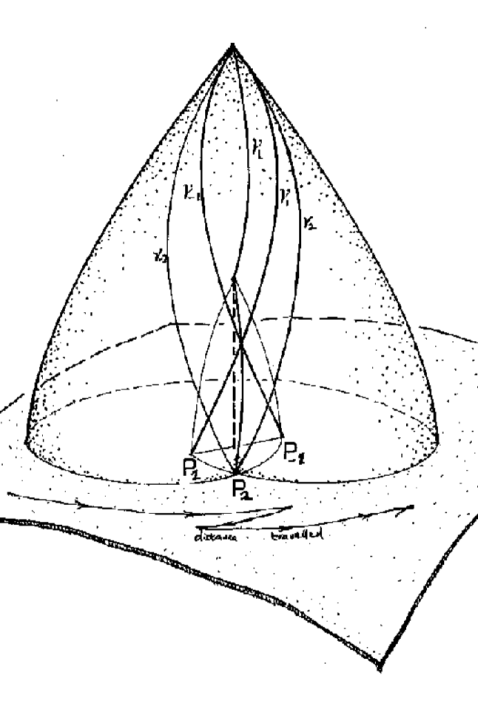
Figure 1: Shape of caustics in past light cone showing preferred geodesics and distance traveled.

Together the radial and transverse equations (15), (9) give the deflection of each null ray relative to the background geometry, and hence the shape of the perturbed light cone in the real lumpy space-time. These deflections are not independent: they are related by the fact that the speed of light is locally unity, so that the actual light path is stationary w.r.t. variation of the arrival time delay. Consequently a sideways deflection (which increases the distance to be traveled) is compensated by an inwards deflection (reducing the distance to be traveled), so the (tangential) lensing equation is a consequence of the (radial) time delay equation (SEF pp.146-147, 170-171). It is this combination of radial and tangential effects, implied by the above equations, that gives the light cone caustics their characteristic shapes (see Figure 1).

3 Angles and Distances

Consider now angles and distances in the perturbed space-time. We start with angular diameter distance. Consider the source plane of a lens in direction $(\vec{\theta})$. Image points of nearby directions will be displaced from their background position $(\ell,\vec{x})$ by the (scaled) displacement $(\Delta\ell,\Delta\vec{\eta})$ $(Z,\vec{y}-\vec{x})=(Z,-\vec{\alpha})$ where the first part is the radial component of the displacement, given by (15), and the second is the tangential component (in the source plane) given by (11). If we move our viewing direction through an arc in the sky, the image point will move; for simplicity we will consider an arc where only one angular component $\theta$ only varies. This gives a 2-dimensional section of the full 3-dimensionalÆ

As we vary $\theta$ through $d\theta$, the (scaled) tangential distance traveled will be $dy^{2}$, and the radial change of distance $dZ^{2}$ will be much less than this. Thus the total distance traveled $DT$ due to an angle increase $\Delta\theta$ is, to good approximation,

$$DT(\Delta\theta)=\int_{\Delta\theta}\,\left|{\frac{\partial y(\theta)}{\partial\theta}}\right|d\theta\;,$$ (19)

where we sum all distances with a positive sign, thus determining the total increment in $|y|$ (see Paper 1). In terms of normalised magnitudes when spherical lensing takes place, the integrand is just $\left|\partial y/\partial\theta\right|=|1-d\alpha/dx|\partial x/\partial\theta.$ By contrast, the background distance is the same expression but with integrand $|\partial x/\partial\theta|$, and Distance gained $DG$ is the distance moved from the starting point:

$$DG(\Delta\theta)=\int_{\Delta\theta}\,{\frac{\partial y(\theta)}{\partial\theta}}\,d\theta~{}=~{}y(\theta)-y(0)\,.$$ (20)

In this case we subtract off those regions where $\partial y/\partial\theta$ is negative, ending up simply with the increment of $y$.

Now when ${\frac{\partial y(\theta)}{\partial\theta}}$ is positive, distance traveled is the same as distance gained. However when ${\frac{\partial y(\theta)}{\partial\theta}}$ changes sign, we have cusps forming (see Paper 1) and in the formula (19) for distance traveled the integral is over the curve corresponding to all values of $\theta$ and hence traverses the cusp backwards and forwards, see Figure 1. This is different from distance gained; the latter is then given by the integral (19) but where now the integral is over the (connected) curve $\gamma$ excluding the cusp sections, so that ${\frac{\partial y(\theta)}{\partial\theta}}$ is positive over all the curve traversed.

The Change in Distance Gained due to the presence of the deflector is small in all cases. The effect for large angular scales does not average to zero when we have a distribution of lenses, but it is very small (the change from the background value is given by the difference of $-D_{ds}\;\vec{\alpha}\,(\vec{\xi})$ at the two ends, corresponding to a minute of arc at most). The Change in Distance Traveled $\Delta DT$ is given by the integral (19), but now taken over all the closed loops $\gamma_{c}$ that are excluded when one calculates distance gained. The effect at each lens is small, but it is cumulative. Hence when there are a large number of lenses, the effect can be large (as discussed in Paper I).

We are also interested in the true Cosmological Area Distance and soÆ the question, as we look over a given solid angle, what area does that cover at the source? This change is given pointwise by the determinant of the lens equation, see (18). We give explicit expressions for this determinant in the following paragraphs. A radial increase of size will be partly compensated by a transverse decrease of size, see e.f. Gunn and Press [6]), so the area distance will not relate very simply to the (radial) angular size distance.

We see then that before caustics form, distance traveled and distance gained are both very similar (and very close to the background value, on large angular scales). Thereafter, they can be very different (as was argued in Paper I). To calculate this, we must locate the cusps and caustics.

3.1 Caustics and Critical Curves

Caustics in a source plane are the points in the plane where the Jacobean of the lensing map is singular. Critical curves are the points in the lensing plane where the light rays pass that will end up at caustics at the source plane. They can be located by determining the zeros of the Jacobean of the lensing map. The set of caustic points in space-time for all source planes form the space-time caustic set.

3.1.1 The Jacobean

Considering a spherical lens ${\bf\hat{L}}$ centered at the origin of the Cartesian $XY$-plane, the Jacobian matrix $J\,=\left(\,\frac{\partial\,\vec{y}}{\partial\,\vec{x}}\,\right)$ of the (transverse) lens mapping in the lens plane has determinant

$$det\,J=\left(1-\frac{\alpha(x)}{x}\right)\,\left(1-\frac{d\alpha(x)}{dx}\right)\;.$$ (21)

(SEF 8.16) which vanishes where either the first or the second brackets on the r.h.s. vanishes.

When the first bracket in (21) vanishes, the radius $x$ is $x_{c}$ such that

$$\frac{m(x_{c})}{x_{c}^{2}}=1~{}~{}\Leftrightarrow~{}~{}\frac{\alpha(x_{c})}{x_{c}}=1~{}~{}\Leftrightarrow~{}~{}\frac{\hat{\alpha}(r_{c})}{r_{c}}=\frac{1}{{\cal R}}\;.$$ (22)

Such a critical point occurs for example at ${\bf r}=(x_{c},0)$; then there is a tangent vector $\Xi_{t}=(0,1)$ to the critical curve at this point, and since the curve is tangential, $\Xi_{t}$ is an eigenvector with zero eigenvalue. Since the tangential critical curves are mapped onto the point $\eta=0$ in the source plane, there exists a caustic there which degenerates to a single point. The equation of the tangential critical curve in two dimensions in the lens plane is then simply $x^{2}=x^{2}_{c}$, where $x_{c}$ solves (22). This corresponds to an Einstein ring [many images, in a circle, of one point in the source plane].

The determinant $det\,J$ in (21) also vanishes where the lastÆ

$$\frac{d\alpha(x_{d})}{dx}=1\;.$$ (23)

This equation describes radial critical curves. Again it corresponds to a circle in the lens plane. It has a radial eigenvector $\Xi_{r}$ with eigenvalue zero. For instance, at ${\bf r}=(\xi,0)$, $\Xi_{r}=(1,0)$. We see in the next section it corresponds to a caustic in the source plane [and a cusp in the surface of constant distance].

3.1.2 The Cross-over and Cusp Angles

The lensing equation (9) is a two-dimensional vector equation with (transverse) components $y_{1}$ and $y_{2}$ while the radial equation gives the 3rd-component for the 2-d section of the past null cone in any surface of constant time. Lensing is radially inward with radial displacement magnitude given by (11). The first term on the right is the position that would have been with no lens; the second term is the effect of the lens.

To express this in terms of the observational angle $\theta$ from the optical axis, we note from the relations $\vec{\xi}=D_{d}\vec{\theta}$, $\vec{x}=\vec{\xi}/\xi_{0}$ that $\vec{x}=D_{d}\vec{\theta}/\xi_{0}$. Hence the magnitude equation takes the form

$$y(\theta)=\frac{D_{d}}{\xi_{0}}\left(\theta-\frac{D_{ds}}{D_{s}}\;\hat{\alpha}\,(D_{d}\theta)\right).$$ (24)

(SEF 4.47b, 5.34). The cusp angles $\theta_{1}$ and $\theta_{-1}$ are determined by

$${\frac{\partial y}{\partial\theta}}|_{\theta_{1}}=0,~{}~{}{\frac{\partial y}{\partial\theta}}|_{\theta_{-1}}=0,$$ (25)

where again by the symmetry, $\theta_{1}=-\theta_{-1}$. Differentiating (24), this occurs when

$$0=D_{s}-D_{ds}{\frac{\partial\hat{\alpha}}{\partial\xi}}(D_{d}\theta_{1})D_{d}$$ (26)

that is

$${\frac{\partial\hat{\alpha}}{\partial\xi}}(D_{d}\theta_{1})={\frac{1}{{\cal R}}}$$ (27)

determines the cusp angle $\theta_{1}$. These angles correspond to the radial critical points in equation (23). In terms of the bending angle diagram (Figure 2), this occurs where the curves $y-x=y_{1}$ are tangent to the curve $\alpha(x)$. The cusp physical size is $D_{s}\theta_{1};$ twice this distance is the difference between distance gained and distance traveled, to good approximation. Æ $\theta_{2}$ and $\theta_{-2}$ are related by

$$y(\theta_{2})=y(\theta_{-2})=0,$$ (28)

where by the spherical symmetry $\theta_{2}=-\theta_{-2}$ and the self-intersection of the light cone (given by the first equality in this equation) occurs on the central line through the lens (as implied by the second equality). Thus we have from ( 24)

$$\theta_{-2}={\frac{D_{ds}}{D_{s}}}\hat{\alpha}(D_{d}\theta_{-2})$$ (29)

determines the cross-over angle $\theta_{-2}$. Thus the cross-over angles $\theta_{2}$ and $\theta_{-2}$ correspond to the critical points satisfying equation (22). In terms of the bending angle diagram (see Figure 2) this occurs where the line $y-x=0$ intersects the curve $\alpha(x)$.

An angle $\theta_{3}$ and corresponding impact parameter $x_{3}$ yields the same image position as the cusp angle, on the other side of the caustic: $y(x_{3})=-y(x_{1})$, and it is this angle that we treat as the cut-off in the caustic size. Henceforth, we refer to this as the cut-off angle $\theta_{3}$ (and the cut-off on the other side occurs at $\theta_{-3}=-\theta_{3}$).

Finally, the maximum deflection caused by the lens occurs when $\theta=\pm\theta_{m}$, where

$${\frac{\partial\hat{\alpha}}{\partial\xi}}(D_{d}\theta_{m})=0$$ (30)

This does not correspond to either of the other angles; indeed it lies between them. For a SCL centred at $\theta=0$, if cusps and cross-overs occur then generically

$$0<\theta_{1}<\theta_{m}<\theta_{2}<\theta_{3}\,.$$

The two-dimensional picture obtained by suppressing one angular coordinate is as shown in Figure 1 (with one radial coordinate and one angular coordinate). Going to the full 3-dimensional picture, at the source plane, the whole picture is circularly symmetric about the optical axis at $\theta=0$. The cross-over angles at $\theta=\pm\theta_{2}$ correspond to a circle in the lens plane but a point (a degenerate caustic) in the source plane; the cusp angles $\theta=\pm\theta_{1}$ correspond to circles in both planes.

We now apply the preceding theory to Top Hat models.

4 The Top-Hat Matter Distribution

density $\delta_{+}$ for $0\leq|\vec{x}|<1$ and a constant outer density $\delta_{-}$ for $1<|\vec{x}|<\lambda$ with $\lambda>1.$ Then the compensation condition (5) is

$$\delta_{-}=-(\lambda^{3}-1)^{-1}\delta_{+}\,,$$ (31)

Unless otherwise stated, we will assume that $\delta_{+}$ is positive (so $\delta_{-}$ is negative). Then the positivity condition (6) demands that

$$0<\delta_{+}<(\lambda^{3}-1)~{}~{}\Leftrightarrow~{}~{}0>\delta_{-}>-1\,,$$ (32)

using the scaled variables, and $\kappa(x)$ will take the form

$$\kappa(x)= C\left(\lambda^{3}\sqrt{1-x^{2}}-\sqrt{\lambda^{2}-x^{2}}\,\right)\,,~{}~{} ~{}~{}0\leq x\leq 1\,,$$ (33)

$$\kappa(x)= -C\sqrt{\lambda^{2}-x^{2}}\,,~{}~{} ~{}~{}1\leq x\leq\lambda\,,$$ (34)

$$\kappa(x)= 0\,,~{}~{} ~{}~{}x>\lambda$$ (35)

where $C=-2\rho_{0}{}\delta_{-}/\sigma_{cr}$, with a central value $\kappa(0)=C\lambda(\lambda^{2}-1)>0$ and a junction value of $\kappa(1)=-C\sqrt{\lambda^{2}-1}<0$. The surface density will positive for $0\leq x<x_{+}<1$, negative for $x_{+}<x<\lambda$, and zero for $\lambda<x$, where

$$x_{+}=\lambda\sqrt{(\lambda^{4}-1)/(\lambda^{6}-1)}\,<1\,.$$ (36)

Substituting into (8) and integrating (12) to find the mass function $m(x)$, we obtain the following:

$$m(x)=Af(x),~{}~{}A=-{\frac{4\rho_{0}}{3}}\delta_{-}{\frac{\xi_{0}\lambda^{3}}{\sigma_{cr}}}\,,$$ (37)

where the function $f(x)$ is given by

$$f(x)= \left(1-{\frac{x^{2}}{\lambda^{2}}}\right)^{3/2}-\left(1-x^{2}\right)^{3/2},~{} ~{}0\leq x\leq 1\,,$$ (38)

$$f(x)= \left(1-{\frac{x^{2}}{\lambda^{2}}}\right)^{3/2},~{} ~{}1\leq x\leq\lambda\,,$$ (39)

$$f(x)= 0,~{} ~{}\lambda\leq x\,.$$ (40)

The function $f(x)$ is a continuous positive even function, with $f(0)=df/dx(0)=0$, a single maximum value of $f(x_{m})=(\lambda^{2}-1)^{3/2}/(\lambda^{6}-1)^{1/2}$ at $x_{m}<1$ given by $x_{m}^{2}=\lambda^{2}(\lambda^{4}-1)/(\lambda^{6}-1)=x_{+}^{2}$, and junction values $f(1)=(\lambda^{2}-1)^{3/2}/\lambda^{3}$, $f(\lambda)=0=df/dx(\lambda)$. Near zero it has the form

$$f(x)={\frac{3}{2}}{\frac{(\lambda^{2}-1)}{\lambda^{2}}}x^{2}-{\frac{3}{8}}\left({\frac{\lambda^{4}-1}{\lambda^{4}}}\right)x^{4}+O(x^{6})\,.$$ (41)

It follows that $m(x)$ is a continuous non-negative function with $m(0)=0$ and junction values $m(\lambda)=0$ and $m(1)=A(\lambda^{2}-1)^{3/2}/\lambda^{3}$. Its maximum value is at $x=x_{m}=x_{+}$, where $m(x_{m})=Af(x_{m})$.

Consequently, because any SCL lens can be built up by a superposition of a sufficient number of top hat lenses, we see that the effective surface deflection mass $M(r)$ is always positive and is exactly zero at the outer edge of the compensating region, that is the effective 2-dimensional surface density $\sigma$ is exactly compensated if the 3-dimensional fractional density $\delta$ is precisely compensated. Hence there is no long-range effect due to the lens: precisely because it is correctly compensated, the deflection angle $\alpha=0$ for impact parameters that lie outside $x=\lambda$ (where the density takes exactly the background value). Thus we note, (1) for compensated lenses, lensing effects occur only for rays that traverse the lens itself and its compensating region; (2) despite the negative values for $\sigma$ at some radii in such a compensated lens, the deflection angle is always positive.

Collecting formulae resulting from (11,12) and (37-40), we have that for a spherically symmetric top-hat matter distribution,

$$\alpha(x)=A\,{\frac{f(x)}{x}},$$ (42)

where the constant is

$$A=\left({\frac{16\pi G\rho_{0}}{3c^{2}}}\right)(\xi_{o}\delta_{+})\left({\frac{\lambda^{3}}{\lambda^{3}-1}}\right){\cal R}\,,$$ (43)

From (22) or (29), cross-overs occur where

$$B(x):={\frac{\alpha(x)}{x}}=1$$ (44)

and from (23) or (27) caustics occur where

$$d\alpha(x)/dx=1\,,$$ (45)

The maximum bending angle $\alpha_{m}$ occurs where $d\alpha/dx=0$.

Consequently,

(1) the bending angle $\alpha(x)$ is a continuous positive odd function with $\alpha(0)=0$, $d\alpha/dx(0)=(3A/2)\left({\frac{\lambda^{2}-1}{\lambda^{2}}}\right)$, a single maximum value $\alpha_{m}$ at $x_{m}<\xi_{0}$ where $x_{m}^{4}={\frac{3\lambda^{4}(\lambda^{2}-1)}{4(\lambda^{6}-1)}}$, and junction values $\alpha(1)=A(\lambda^{2}-1)^{3/2}/\lambda^{3}$, $\alpha(\lambda)=0=d\alpha/dx(\lambda)$.

(2) its slope $d\alpha(x)/dx$ is an even continuous function with maximum value $d\alpha(0)/dx=(3A/2\lambda^{2})(\lambda^{2}-1)$ at the centre, positive from $x=0$ to $x_{m}$, negative from $x=x_{m}$ to $\lambda$, and zero thereafter, with junction values $d\alpha(1)/dx=-(A/\lambda^{3})(\lambda^{2}+2)\sqrt{\lambda^{2}-1}$ (here it takes its minimum value and its derivative $d/dx(d\alpha/dx)$ is discontinuous, diverging from the left but finite on the right) and $d\alpha(\lambda)/dx=0$. Hence caustics occur iff

$$(3A/2\lambda^{2})(\lambda^{2}-1)\equiv A_{crit}>1$$ (46)

(with a degenerate case when equality occurs). If they occur, say at $x=x_{2}$ , then $0<x_{2}<1$ and $x_{2}$ satisfies

$${\frac{d\alpha(x_{2})}{dx}}={\frac{A}{x_{2}^{2}}}\left[(1+2x_{2}^{2})\sqrt{1-x_{2}^{2}}-(1+{\frac{2x_{2}^{2}}{\lambda^{2}}})\sqrt{1-{\frac{x_{2}^{2}}{\lambda^{2}}}}\right]=1\,,$$ (47)

with the corresponding angle $\theta_{2}$ given by $\theta_{2}=x_{2}\xi_{0}/D_{d}$.

(3) The function $B(x)=\alpha(x)/x=Af(x)/x^{2}$ (with $f(x)$ given by (38-40)) is even, positive, monotonic decreasing, and continuous, with a maximum value $B(0)=(3A/2\lambda^{2})(\lambda^{2}-1)$ at the centre, and junction values $B(1)=(A/\lambda)(\lambda^{2}-1)^{3/2}/\lambda\,$, $B(\lambda)=0$. Hence cross-overs also occur iff ( 46) is satisfied. They can occur for any value of $x>x_{2}$ up to $\lambda$. If they occur, say at $x=x_{1}$, then

$$Af(x_{1})/x_{1}^{2}=1\,.$$ (48)

with the corresponding angle $\theta_{1}$ given by $\theta_{1}=x_{1}\xi_{0}/D_{d}$, where $f(x)$ is given either by (38) (if $x_{1}<1$) or by (39) (if $1<x_{1}<\lambda$) (one cannot tell a priori in which range it will lie; one has to try to solve one, and if there is no solution, solve the other). Then $\theta_{2}(z_{d},z_{s})$ is the angle determining how large a part of the sky is covered by the Einstein circle corresponding to the cross-over surface $z=z_{s}$ for lenses at $z_{d}$ (giving multiple images of the central point at $z_{s}$). How this scales with $z_{d}$ (for given $z_{s}$) depends on how $\rho_{0}$, $\xi_{0}$, $\delta_{+}$, $\lambda$ and ${\cal R}$ scale with $z_{d}$.

(4) Pointwise over the image, the area shrinking factor is given by $\beta=|det\,J|$ given by (21). This can be evaluated from the formulae given above. Using the expansion (41) one can evaluate this determinant near the centre-line $\theta=0$; the result is

$$det\,J=\left(1-A_{crit}\right)+O(x^{2})$$ (49)

which is $1$ near the lens (when $A$ is small) and goes to $-A_{crit}$ (see (46)) when $A$ is large (the minus sign because images are reversed).

We can determine a value for the lensing parameter $M_{0}$ either by directly estimating the quantities in the definition (43), or by estimating the maximum bending angle $\alpha_{m}$ for lenses considered. For example, if $\lambda=2$, the r.h.s. of (42) has a maximum value of $0.70A$ (when $x=0.87$). From (43) with the bending angle relation (42) and angle scaling relation (10) we see that then $M_{0}$ is determined by the relation

$$M_{0}\times 1.14\times 0.7={\frac{2c}{H_{0}}}{\frac{\alpha_{m}}{\xi_{0}}}\,.$$ (50)

Æ

4.1 Results

We have written a series of Truebasic programmes that compute all the relevant quantities for Tophat lenses, as functions of (i) the determining parameter $A$, (ii) the source redshift $z_{s}$ for fixed lens redshift $z_{d}$, (iii) the lens redshift $z_{d}$ for fixed source redshift $z_{s}$. We have experimented with parameter values that correspond to observed gravitational lensing systems; some of the results are given in the following tables and in Figures 3 to 5. This area shrinking ratio is about 3 after cusps have occurred, for scales of about 3 times the cusp scale, corresponding to the cusp image point where the deflection is the same size as at the cusp.

4.2 Galaxy clusters

We present a table of results for parameters corresponding to four well-known galaxy clusters that cause gravitational lensing (note that we are not making detailed models of these objects; rather we are using their observed properties to determine reasonable parameter values in our SCL model). From the cluster Abell $2218$ (see refs. [7, 8]) we have selected as images the arcs at redshifts $z_{s}=2.6$ and $3.3\;$ respectively, as a case study, where the brackets imply this is evaluated at the angle cut-off angle. We then list the corresponding shrinking factor $\left\langle\beta\right\rangle$ for these two images, at the cut-off angle, followed by their cusp and cross-over angles. The last column is the shrinking factor for the source placed at decoupling redshift $z_{s}=1200$ . We also consider other lensing clusters Abell $963$ (ref. [12] ), Abell $370$ (refs. [11, 21]), and Abell $2390$ (refs. [19, 21]).

LENS $$\alpha_{max}$$

LENS

Cusp angle

$$\theta_{2}$$

4.3 Galaxies

We have also used a set of galactic lenses, as evidenced by multiple images of more distant objects, to provide parameters for our model, giving the second table. The first lens is often referred to as the ‘clover leaf’: $+H1413+117$ has four images of a QSO at redshift $z_{d}=2.55\;$(See refs. [17, 22]). The second is the seen in QSO images A and B for the system $2345+007$ correspond to a redshift $z_{d}=2.15$, despite image A being $1.7mag$ brighter than image B (ref. [18, 23]). The third is the triple radio source $+MG2016+112$ (see ref. [15]). The fourth is the QSO pair in $1635+267$ with nearly equal redshift $z_{d}=1.96$ [14]. Finally a nearly full Einstein ring was observed in $+MG1131+0456$, albeit somewhat elliptic in shape (ref. [9] ).

LENS $$\alpha_{max}$$

shrinking

LENS

Cusp angle

$$\theta_{2}$$

We find that the caustics shrinking factor tends to an average factor $>3$ at large z (as required to get a 3-fold covering factor). However because of the divergence of the light rays within the cusps, it can be much larger for parameter values implying to strong lensing (the actual angle corresponding to the cusps is then much smaller than in the equivalent FL model).

5 Conclusions

Of particular interest is the way the cusp size and the “shrinking” vary with redshift of the source and of the lensing object. This depends on two things: firstly the variation of angular sizes with redshift, remembering (a) minimum angular apparent diameter occurs at $z=1.25$, so that the maximum angle $\theta_{c}$ for cusps to form due to lenses of given size and strength will have minimum at that redshift; and (b) that the ratio of distances that enters $\sigma_{cr}$ saturates with increasing $z_{s}$ (for given $z_{d}$) but has a maximum for each $z_{s}$ at a $z_{d}$ of about $0.6$ which is thus the optimal distance for the lens in order to create cusps on the last scattering surface. Æ that are not typical of all galaxies or clusters; but they confirm in a concrete way the broad picture proposed in Paper I: an area ‘shrinking’ factor of 3 will occur for each lens that causes cusps, on the scale of the cusps (precisely: at the cut-off angle $\theta_{3}$ which gives the same deflection at the source as the cusp angle, but on the opposite side). The total effect when averaging over large angular scales will depend on what fraction of the sky is covered by these angles for all lenses at all smaller scales, as a function of redshift; some simple estimates of this overall effect were given in Paper I. To determine realistic multiplicity factors as a function of redshift will require simulations with multiple lensing and more realistic lens models, for example standard elliptical lens models determined by a velocity dispersion parameter and ellipticity parameters as in [7] which allow an increase in the degree of multiple covering (because individual elliptic lenses can have a covering factor of 5). The effect will differ on angular scales, and will almost certainly be substantial due to micro-lensing, with an additional increase due to galactic and cluster lensing. The implication of this paper and Paper I is that it is incorrect to assume that areas average out to the background FL value on large angular scales; one can only know the true area ratios - expressed in the shrinking factors considered in this paper - by detailed calculation.

Figure 2: The bending angle diagram for two different redshifts. (a) one large, so other side of conjugate point Q; (b) One small, so this side of conjugate point Q. The number of images is the number of times the line y = x intersects the bending angle curve. Considering curve (a), firstly, there is one image corresponding to line (c); then there are two images for line (d) which is tangent to the curve and determines the cusp angle; there are three intersections for line (e) which determines the cross-over angles (as it corresponds to no displacement at the source plane); there are 3 images for generic position (f), again two images for line (g) as it passes through the cusp, and finally one image for line (h). Parameters based on the lens +MG1131+0456.

Figure 3: Variation in (a) cusp angle, (b) the crossover angle, and (c) the cut-off angle. The image redshift starts at the limiting value of $z_{s}=z_{d}=0.231$, and increases through the arc redshift of 0.914, up to the value $z_{s}=5$. Parameters based on the lens A2390.

Figure 4: The pointwise area shrinking ratio $\gamma$ for parameters based on the lens +MG1131+0456.

Figure 5: The average area distance shrinking ratio $\beta$ for the Abell cluster 2390. The average $\langle\beta\rangle$ at (a) $\theta=\theta_{1}$ (the cusp angle), (b) $\theta=\theta_{2}$ (the cross-over angle), and (c) $\theta=\theta_{3}$ (the cut-off angle).

References

- [1] G. F. R. Ellis, B. A. C. C. Bassett, and P. K. S. Dunsby: Lensing and caustic effects on cosmological distances. To appear, Class Quant Grav, gr-qc/9801092 (1997).
- [2] S. Weinberg, Ap. J, 208, L1, (1976).
- [3] N. Mustapha, B.A.C.C. Bassett, C. Hellaby, and G F R Ellis: The Distortion of The Area Distance-Redshift Relation in Inhomogeneous Isotropic Universes. To appear, Class Quant Grav, gr-qc/9708043 (1997).
- [4] P. Schneider, J. Ehlers and E. E. Falco: Gravitational Lenses. (Springer-Verlag, Berlin, 1992).
- [5] G F R Ellis and M Jaklitsch, Astrophys. Journ. 346, 601-606 (1989).
- [6] W. H. Press and J. E. Gunn, Ap. J., 185, 397 (1973).
- [7] J.-P. Kneib, R.S. Ellis, I. Smail, W.J.Couch, and R. M. Sharples, Ap J 471: 643-656, 1996.
- [8] R. Pello-Descayre, G. Soucail, B. Sanahuja, G. Mathez, and E. Ojero, Astrophys. 190, L11-L14 (1988).
- [9] J.N. Hewitt, E.L. Turner, D.P. Schneider, B.F. Burke, G.I. Langston, and C.R. Lawrence, Nature, 333, 537 (1988) ; J.N. Hewitt, B.F. Burke, E.L. Turner, D.P. Schneider, C.R. Lawrence, G.I. Langston, and J.P. Brody, in [10].
- [10] J.M. Moran, J.N Hewitt, and K.Y.Lo: Gravitational lenses. Lecture Notes in Physics, 330, Springer-Verlag (1989).
- [11] G. Soucail, Y. Mellier, B. Fort, G. Mathez, and M. Cailloux, Astr. Ap., 191, L19 (1988).
- [12] R.J. Lavery, and J.P. Henry, Ap. J., 329, L21 (1988).
- [13] E. Kellog, E.E Falco, W. Forman, C. Jones, and P. Slane, in [20].
- [14] S. Djorgovsky, and H. Spinrad, Ap. J., 282 , L1 (1984).
- [15] C.R. Lawrence, D.P. Schneider, M. Schmidt, C.L. Bennett, J.N. Hewitt, B.F. Burke, E.L. Turner, and J.E Gunn, Science, 223, 46 (1984).
- [16] J. Huchra, M. Gorenstein, S. Kent, I. Shapiro, G. Smith, E. Horine, and R. Perley, Astron. J., 90, 691 (1985).
- [17] P. Magain, J. Swings, J.-P., U. Borgeest, R. Kayser, H. Kühr, S. Refsdal, and M. Remy, Nature, 334, 327 (1988).
- [18] D.W. Weedman, R.J. Weymann, R.F. Green, and T.M. Heckman, Ap. J., 255, L5 (1982).
- [19] B. Fort, in [20].
- [20] Y. Mellier, B. Fort, and G. Soucail, Gravitational Lensing Lecture Notes in Physics, 360, Springer-Verlag.
- [21] Y. Mellier, G. Soucail, B. Fort, J.-F. Le Borgne, and R. Pello, in [20].
- [22] R. Kayser, J. Surdej, J.J. Condon, K.I. Kellermann, P. (1990).
- [23] C.C. Stidel, and W.L.W. Sargent, Astron. J., 99, 1693 (1990).