On the gravitational, dilatonic and axionic radiative damping of cosmic strings

Abstract

We study the radiation reaction on cosmic strings due to the emission of dilatonic, gravitational and axionic waves. After verifying the (on average) conservative nature of the time-symmetric self-interactions, we concentrate on the finite radiation damping force associated with the half-retarded minus half-advanced “reactive” fields. We revisit a recent proposal of using a “local back reaction approximation” for the reactive fields. Using dimensional continuation as convenient technical tool, we find, contrary to previous claims, that this proposal leads to antidamping in the case of the axionic field, and to zero (integrated) damping in the case of the gravitational field. One gets normal positive damping only in the case of the dilatonic field. We propose to use a suitably modified version of the local dilatonic radiation reaction as a substitute for the exact (non-local) gravitational radiation reaction. The incorporation of such a local approximation to gravitational radiation reaction should allow one to complete, in a computationally non-intensive way, string network simulations and to give better estimates of the amount and spectrum of gravitational radiation emitted by a cosmologically evolving network of massive strings.

I Introduction

Cosmic strings are predicted, within a wide class of elementary particle models, to form at phase transitions in the early universe [1], [2]. The creation of a network of cosmic strings can have important astrophysical consequence, notably for the formation of structure in the universe [3], [4]. A network of cosmic strings might also be a copious source of the various fields or quanta to which they are coupled. Oscillating loops of cosmic string can generate observationally significant stochastic backgrounds of: gravitational waves [5], massless Goldstone bosons [6], light axions [7], [8], or light dilatons [9]. The amount of radiation emitted by cosmic strings depend: (i) on the nature of the considered field; (ii) on the coupling parameter of this field to the string; (iii) on the dynamics of individual strings; and (iv) on the distribution function and cosmological evolution of the string network. It is important to note that the latter network distribution function in turn depends on the radiation properties of strings. Indeed, numerical simulations suggest that the characteristic size of the loops chopped off long strings at the epoch $t$ will be on order of the smallest structures on the long strings, which is itself arguably determined by radiative back reaction [10], [11]. For instance, if one considers grand unified theory (GUT) scale strings, with tension $\mu\sim\Lambda_{\rm GUT}^{2}$, gravitational radiation (possibly together with dilaton radiation which has a comparable magnitude [9]) will be the dominant radiative mechanism, and will be characterized by the coupling parameter $G\mu\sim(\Lambda_{\rm GUT}/m_{\rm Planck})^{2}\sim 10^{-6}$. It is then natural to expect that the same dimensionless parameter $G\mu$ will control the radiative decay of the small scale structure (crinkles and kinks) on the horizon-sized strings, thereby determining also the characteristic size relative to the horizon of the small loops produced by the intersections of long strings: $\ell_{\rm loops}\equiv\widehat{\alpha}\,ct$, with $\widehat{\alpha}\sim\Gamma_{\rm kink}\,G\mu$, $\Gamma_{\rm kink}$ being some dimensionless measure of the network-averaged radiation efficiency of kinky strings [10], [11], [12], [13]. If one considers “global” strings, i.e. strings formed when a global symmetry is broken at a mass scale $f_{a}$, emission of the Goldstone boson associated to this symmetry breaking will be the dominant radiation damping mechanism and will be characterized by the dimensionless parameter $f_{a}^{2}/\mu_{\rm effective}\sim(\log(L/\delta))^{-1}\sim 10^{-2}$, where the effective tension $\mu_{\rm effective}$ is renormalized by a large logarithm (see, e.g., [2]).

Present numerical simulations of string networks do not take into account the effect of radiative damping on the actual string motion. The above mentioned argument concluding in the case of GUT strings to the link $\widehat{\alpha}\sim\Gamma_{\rm kink}\,G\mu$ between the loop size and radiative effects has been justified by Quashnock and Spergel [11] who studied the gravitational back reaction of a sample of cosmic string loops. However, their “exact”, non-local approach to gravitational back reaction is numerically so demanding that there is little prospect to implementing it in full string network simulations. This lack of consideration of the dynamical effects of radiative damping is a major deficiency of string network simulations which leaves unanswered crucial questions such as: Is the string distribution function attracted to a solution which “scales” with the horizon size down to the smallest structures? and What is the precise amount and spectrum of the gravitational (or axionic, in the case of global strings) radiation emitted by the combined distribution of small loops and long strings?

Recently, Battye and Shellard [14], [15] proposed a new, computationally much less intensive, approach to the radiative back reaction of (global) strings. They proposed a “local back reaction approximation” based on an analogy with the well-known Abraham-Lorentz-Dirac result for a self-interacting electron. Their approach assumes that the dominant contribution to the back reaction force density at a certain string point comes from string segments in the immediate vicinity of that point. They have endeavored to justify their approach by combining analytical results (concerning approximate expressions of the local, axionic radiative damping force) and numerical simulations (comparison between the effect of their local back reaction and a direct field-theory evolution of some global string solutions).

In this paper, we revisit the problem of the back reaction of cosmic strings associated to the emission of gravitational, dilatonic and axionic fields, with particular emphasis on the “local back reaction approximation” of Battye and Shellard. Throughout this paper, we limit our scope to the self-interaction of Nambu strings, in absence of any non-trivial external fields. This problem can be (formally) treated by a standard perturbative approach, i.e. by expanding all quantities in powers of the gravitational coupling constant $G$. We work only to first-order in $G$. To this order, we first verify the fact (well-known to hold for self-interacting, electrically charged, point particles [16]) that the time-symmetric part of the self-interaction (i.e. the part mediated by the half-retarded plus half-advanced Green function) is, on the average, conservative, i.e. that it does not (after integration) drain energy-momentum out of the string. As we are interested in radiation damping, this allows us to concentrate on the time-odd part of the self-interaction, mediated by the half-retarded minus half-advanced Green function. This “reactive” part of the self-interaction is (as in the case of point charges) finite. [By contrast, the time-symmetric self-interaction is (formally) ultraviolet divergent. This divergence is not of concern for us here because, as shown in Refs. [17], [18] and further discussed below, its infinite part is renormalizable, and, as said above, its finite part does not globally contribute to damping.] Contrary to the case of point charges, the reactive part is non-local, being given by an integral over the string. Following Battye and Shellard [14], [15] we study the “local approximation” to this reaction effect. We find very convenient for this study to use the technique of dimensional continuation (well-known in quantum field theory).

In the case of the axionic self-field, we find that the axionic reaction force defined by the “local back reaction approximation” of Ref. [14] leads to antidamping rather than damping, as claimed in Refs. [14], [15]. We also investigate below the corresponding local approximations to gravitational and dilatonic self-forces and find zero damping in the gravitational case, and a normal, positive damping for the dilatonic case. The physical origin of these paradoxical results is explained below (Sec. IV F) by tracing them to the modification of the field propagator implicitly entailed by the use of the local back reaction approximation. We show that, in the case of gauge fields, this modification messes up the very delicate sign compensations which ensure the positivity of the energy carried away by gauge fields. Thereby, one of the main results of the present work is to prove the untenability of applying a straightforward local back reaction approximation to gauge fields such as gravitational and axionic fields. However, this untenability does not necessarily apply to the case of non-gauge fields. Indeed, our work proves that the application of this local approximation to the dilatonic field (which is not a gauge field) leads to the correct sign for damping effects. In this non-gauge field case, the argument (of Sec. IV F) which showed the dangers of approximating the field propagator for gauge fields, looses its strength. This leaves therefore open the question of whether the “local approximation” to dilatonic back reaction might define (despite its shortcomings discussed below) a phenomenologically acceptable approximation to the exact, non-local self-force. In this direction, we give several arguments, and strengthen them by some explicit numerical calculations, toward showing that the meaningful (positive-damping) dilatonic local back reaction force can be used, after some modification, as a convenient effective substitute for the exact (non-local) gravitational back reaction force.

This phenomenological proposal is somewhat of an expedient because it rests on an “approximation” whose validity domain is severely limited. However, pending the discovery of a better local proposal, we think that the incorporation of our proposed local reaction force (171) should allow one to complete, in a computationally non-intensive way, string network simulations and to give better estimates of the amount and spectrum of gravitational radiation emitted by a cosmologically evolving network of massive strings.

In the next section, we present our formalism for treating self-interactions of strings. We describe in Section III our results for the renormalizable, divergent self-action terms, and, in Section IV, our results for the finite contributions to the “local” reaction force. In Section V we indicate how the local dilatonic damping force could be used in full-scale network simulations to simulate the dynamical effects of gravitational radiation. Section VI contains our conclusions. Some technical details are relegated to the Appendix.

As signs will play a crucial role below, let us emphasize that we use the “mostly positive” signature $(-,+,+,+)$ for the space-time metric $g_{\mu\nu}$ ($\mu,\nu=0,1,2,3$), and the corresponding $(-,+)$ signature for the worldsheet metric $\gamma_{ab}$ ($a,b=0,1$ being worldsheet indices).

II Cosmic strings interacting with gravitational, dilatonic and axionic fields

We consider a closed Nambu string $z^{\mu}(\sigma^{a})$ (with $\sigma^{0}=\tau$, $\sigma^{1}=\sigma$, $0\leq\sigma<L$) interacting with its own gravitational $g_{\mu\nu}(x^{\lambda})\equiv\eta_{\mu\nu}+h_{\mu\nu}(x^{\lambda})$, dilatonic $\varphi(x)$, and axionic (Kalb-Ramond) $B_{\mu\nu}(x)$ fields. The action for the string coupled to $g_{\mu\nu}$, $\varphi$ and $B_{\mu\nu}$ reads

$$S_{s}=-\int\mu(\varphi)\,dA-\frac{\lambda}{2}\int B_{\mu\nu}\,dz^{\mu}\wedge dz^{\nu}\,.$$ (1)

Here $dA=\sqrt{\gamma}\,d^{2}\,\sigma$ (with $\gamma\equiv-\det\gamma_{ab}$; $\gamma_{ab}\equiv g_{\mu\nu}(z)\,\partial_{a}\,z^{\mu}\,\partial_{b}\,z^{\nu}$ denoting the metric induced on the worldsheet) is the string area element and the dilaton dependence of the string tension $\mu$ can be taken to be exponential

$$\mu(\varphi)=\mu\,e^{2\alpha\varphi}\,.$$ (2)

At the linearized approximation where we shall work the form (2) is equivalent to a linear coupling $\mu(\varphi)\simeq\mu(1+2\alpha\varphi)$. The dimensionless parameter $\alpha$ measures the strength of the coupling of $\varphi$ to cosmic strings (our notation agrees with the tensor-scalar notation of Ref. [19]), while the coupling strength of the axion field is measured by the parameter $\lambda$ with dimension $({\rm mass})^{2}$. Due to our “gravitational normalization” of the kinetic term of $B_{\mu\nu}$, the link between $\lambda$ and the mass scale $f_{a}$ used in Refs. [14], [15] is $2G\,\lambda^{2}=\pi f_{a}^{2}$.

The action for the fields is

$$S_{f}=\frac{1}{16\pi G}\,\int d^{4}x\sqrt{g}\,\left[{\cal R}-2\,\nabla^{\mu}\varphi\,\nabla_{\mu}\varphi-\frac{1}{12}\,e^{-4\alpha\varphi}\,H_{\mu\nu\rho}\,H^{\mu\nu\rho}\,\right]\,,$$ (3)

where $H_{\mu\nu\rho}=\partial_{\mu}\,B_{\nu\rho}+\partial_{\nu}\,B_{\rho\mu}+\partial_{\rho}\,B_{\mu\nu}$, $g\equiv-\det\,(g_{\mu\nu})$, and where we use the curvature conventions ${\cal R}^{\mu}_{\,\,\,\,\nu\rho\sigma}=\partial_{\rho}\Gamma^{\mu}_{\nu\sigma}-\dots\,,\,\,{\cal R}_{\mu\nu}={\cal R}^{\rho}_{\,\,\,\,\mu\rho\nu}$. With this notation, a tree-level coupled fundamental string (of string theory) has $\alpha=1$ (in 4 dimensions) and $\lambda=\mu$.

Everywhere in this paper, we shall assume the absence of external fields. More precisely, the background values of the fields we consider are $g_{\mu\nu}^{0}=\eta_{\mu\nu}$, $\varphi^{0}=0$, $B_{\mu\nu}^{0}=0$. Our results are derived only for this case, by using (formal) perturbation theory around these trivial backgrounds. It is however understood, as usual, that one can later (e.g. for cosmological applications) reintroduce a coupling to external fields, varying on a scale much larger than the size of the string, by suitably covariantizing the final, trivial-background results derived here. Such an approximate treatment should be sufficient for the cosmological applications we have in mind. On the other hand, the methods used here are not appropriate for treating the general case of a string interacting with external gravitational and dilatonic fields of arbitrary strength and spacetime variability. To treat such a case, one would need a more general formalism, such as that of Ref. [20]. Note, however, that the straightforward, non-explicitly covariant, perturbation approach to radiation damping effects used here is the string analog of all the standard work done on the gravitational radiation damping of binary systems (see, e.g., [21] for a review).

In other words, our aim in this paper is to derive, consistently at the first order in the basic coupling constant $G$ (see Eq. (3)), both the fields generated by the string,

$$h_{\mu\nu}(x)\equiv g_{\mu\nu}(x)-\eta_{\mu\nu} = G\,h_{\mu\nu}^{1}(x)+{\cal O}(G^{2})\,,\quad\quad\varphi(x)=0+G\,\varphi^{1}(x)+{\cal O}(G^{2})\,,$$ (5)

$$B_{\mu\nu}(x)=0+G\,B_{\mu\nu}^{1}(x)+{\cal O}(G^{2})\,,$$

and the (non-covariant) explicit form of the string equations of motion, written in a specified  (class of) worldsheet gauge(s),

$$\mu\,\eta_{\mu\nu}\,(\ddot{z}^{\nu}-z^{\prime\prime\nu})=G\,{\cal F}_{\mu}^{1}+{\cal O}(G^{2})\,.$$ (6)

The string action (1) can be written (using the Polyakov form) as

$$S_{\rm s}=-\frac{\mu}{2}\,\int d^{2}\sigma\,e^{2\alpha\,\varphi}\,\sqrt{\widehat{\gamma}}\,\widehat{\gamma}^{ab}\,\partial_{a}z^{\mu}\,\partial_{b}z^{\nu}\,g_{\mu\nu}-\frac{\lambda}{2}\,\int d^{2}\sigma\epsilon^{ab}\,\partial_{a}z^{\mu}\,\partial_{b}z^{\nu}\,B_{\mu\nu}\,,$$ (7)

where the worldsheet metric $\widehat{\gamma}_{ab}$ must be independently varied and where $\epsilon^{01}=-1$, $\epsilon^{10}=1$. The equation of motion of $\widehat{\gamma}_{ab}$ is the constraint that it be conformal to the induced metric $\gamma_{ab}=g_{\mu\nu}(z)\,\partial_{a}\,z^{\mu}\,\partial_{b}\,z^{\nu}$. In the following, we shall often use the conformal gauge $\sqrt{\widehat{\gamma}}\,\widehat{\gamma}^{ab}=\sqrt{\gamma}\,\gamma^{ab}=\eta^{ab}$ (where $\eta^{00}=-1$, $\eta^{11}=+1$), i.e. we shall choose the $(\tau,\sigma)$ parametrization of the worldsheet so that

$$\dot{z}^{\mu}\,\dot{z}^{\nu}\,g_{\mu\nu}+z^{\prime\,\mu}\,z^{\prime\,\nu}\,g_{\mu\nu}=0\,,\quad\quad\dot{z}^{\mu}\,z^{\prime\,\nu}\,g_{\mu\nu}=0\,.$$ (8)

Here $\dot{z}\equiv\partial_{0}\,z\equiv\partial\,z/\partial\,\tau$ and $z^{\prime}\equiv\partial_{1}\,z\equiv\partial\,z/\partial\,\sigma$. Note also the expression, in this gauge, of the worldsheet volume density

$$\sqrt{\gamma}=g_{\mu\nu}\,z^{\prime\,\mu}\,z^{\prime\,\nu}=-g_{\mu\nu}\,{\dot{z}}^{\mu}\,{\dot{z}}^{\nu}\,.$$ (9)

Let us note that the string contribution to the energy-momentum tensor,

$$T^{\mu\nu}=\frac{2}{\sqrt{g}}\,\frac{\delta S_{m}}{\delta g_{\mu\nu}}\,,$$ (10)

reads

$$T^{\mu\nu}=\frac{\mu}{\sqrt{g}}\,\int d^{2}\sigma\,e^{2\alpha\,\varphi}\,U^{\mu\nu}\,\delta^{4}(x-z(\sigma))\,,$$ (11)

where $\int d^{4}x\,\delta^{4}(x)=1$ and

$$U^{\mu\nu}\equiv-\sqrt{\gamma}\,\gamma^{ab}\,\partial_{a}\,z^{\mu}\,\partial_{b}\,z^{\nu}={\dot{z}}^{\mu}\,{\dot{z}}^{\nu}-z^{\prime\,\mu}\,z^{\prime\,\nu}\qquad\hbox{(in conformal gauge)}$$ (12)

is the “vertex operator” for the interaction of the string with the gravitational field $g_{\mu\nu}$. [The vertex operators used here are the $x$-space counterparts of the $k$-space vertex operators used in quantum string theory, e.g. $\widehat{U}^{\mu\nu}(k)=\int d^{2}\sigma\,U^{\mu\nu}(z(\sigma))\,\exp(i\,k_{\lambda}\,z^{\lambda}(\sigma))$.] The corresponding vertex operator for the interaction with the dilaton $\varphi$ is simply the trace $U\equiv g_{\mu\nu}\,U^{\mu\nu}$, while the one corresponding to the axion $B_{\mu\nu}$ is

$$V^{\mu\nu}\equiv-\epsilon^{ab}\,\partial_{a}\,z^{\mu}\,\partial_{b}\,z^{\nu}={\dot{z}}^{\mu}\,z^{\prime\nu}-{\dot{z}}^{\nu}\,z^{\prime\mu}\,.$$ (13)

The exact equation of motion of the string can be written (in any worldsheet gauge) as

$$0=\frac{\delta S_{s}}{\delta z^{\mu}}\equiv\mu\,g_{\mu\nu}\,e^{2\alpha\varphi}\,\partial_{a}(\sqrt{\gamma}\,\gamma^{ab}\,\partial_{b}z^{\mu})+{\Phi}_{\mu}\,,$$ (14)

where the quantity ${\Phi}_{\mu}$ is defined by

$${\Phi}_{\mu}\equiv{\Phi}_{\mu}^{\varphi}+{\Phi}_{\mu}^{h}+{\Phi}_{\mu}^{B}\,,$$ (15)

with

$${\Phi}_{\mu}^{\varphi} = \mu\,\alpha\,e^{2\alpha\varphi}\,U\,\partial_{\mu}\varphi-2\mu\,\alpha\,e^{2\alpha\varphi}\,g_{\mu\alpha}\,U^{\alpha\beta}\,\partial_{\beta}\varphi\,,$$ (16)

$$\vrule width=0.0pt,height=27.0pt,depth=15.0pt{\Phi}_{\mu}^{h} = -\mu\,e^{2\alpha\varphi}\,g_{\mu\nu}\,\Gamma_{\alpha\beta}^{\nu}\,U^{\alpha\beta}=\frac{\mu}{2}\,e^{2\alpha\varphi}\,U^{\alpha\beta}\,\partial_{\mu}h_{\alpha\beta}-\mu\,e^{2\alpha\varphi}\,U^{\alpha\beta}\,\partial_{\alpha}h_{\beta\mu}\,,$$ (17)

$${\Phi}_{\mu}^{B} = \frac{\lambda}{2}\,V^{\alpha\beta}\,H_{\mu\alpha\beta}=\frac{\lambda}{2}\,V^{\alpha\beta}\,\partial_{\mu}B_{\alpha\beta}+\lambda\,V^{\alpha\beta}\,\partial_{\alpha}B_{\beta\mu}\,.$$ (18)

Let us emphasize that, while ${\Phi}_{\mu}^{\varphi}$ and ${\Phi}_{\mu}^{B}$ are well defined, spacetime and worldsheet covariant objects, ${\Phi}_{\mu}^{h}$, by contrast, is not a covariantly defined object (but the full combination $\delta S_{s}/\delta z^{\mu}$ of Eq. (14) is a covariant object). It can be noted that the sum of the dilatonic and gravitational contributions (16), (17) simplify if they are expressed in terms of the string metric $g_{\mu\nu}^{s}\equiv e^{2\alpha\varphi}\,g_{\mu\nu}$ to which the string is directly coupled. Indeed,

$${\Phi}_{\mu}^{h}+{\Phi}_{\mu}^{\varphi}=-\mu\,g^{s}_{\mu\nu}\,\Gamma_{\alpha\beta}^{\nu}[g^{s}_{\rho\sigma}]\,U^{\alpha\beta}=\frac{\mu}{2}\,U^{\alpha\beta}\,\partial_{\mu}g^{s}_{\alpha\beta}-\mu\,U^{\alpha\beta}\,\partial_{\alpha}g^{s}_{\beta\mu}\,.$$ (19)

Except when otherwise specified, we shall henceforth work in the conformal gauge associated to the actual metric in which the string evolves (and not the conformal gauge associated to, say, a flat background metric $\eta_{\mu\nu}$). In this gauge the equations of motion of the string read

$${\cal E}_{\mu}=0,\quad\mbox{with }\quad{\cal E}_{\mu}\equiv\mu\,g^{s}_{\mu\nu}\,\eta^{ab}\,\partial_{ab}z^{\nu}+{\Phi}_{\mu}\equiv-\mu\,g^{s}_{\mu\nu}\,(\ddot{z}^{\nu}-z^{\nu\,\prime\prime})+{\Phi}_{\mu}\,.$$ (20)

When using this gauge, one must remember that the constraints (8) [which read the same when written in terms of the string metric $g^{s}_{\mu\nu}$] involve the metric. These constraints read (in terms of the string metric)

$$T_{ab}^{s}=0,\quad\mbox{with}\quad T_{ab}^{s}\equiv g^{s}_{\mu\nu}(z)\,\partial_{a}\,z^{\mu}\,\partial_{b}\,z^{\nu}-\frac{1}{2}\,\eta_{ab}\,\eta^{cd}\,g^{s}_{\mu\nu}(z)\,\partial_{c}\,z^{\mu}\,\partial_{d}\,z^{\nu}\,.$$ (21)

The constraints $T_{ab}^{s}=0$ are preserved by the (gauge-fixed) evolution (20). Indeed, it is easy to check the identity

$$\eta^{ab}\,\partial_{a}T_{bc}^{s}\equiv\partial_{c}z^{\mu}\,(g_{\mu\nu}^{s}\,\eta^{ab}\,\partial_{ab}z^{\nu}+{\Phi}_{\mu}^{\varphi}+{\Phi}_{\mu}^{h})\equiv\partial_{c}z^{\mu}\,{\cal E}_{\mu}\,.$$ (22)

In the last step of Eq. (22) we used the algebraic identity $\partial_{c}z^{\mu}\,{\Phi}_{\mu}^{B}\equiv 0$. When the gauge-fixed equations of motion are satisfied, i.e. when ${\cal E}_{\mu}=0$, the constraints satisfy the conservation law $\eta^{ab}\,\partial_{a}T^{s}_{bc}=0$. This conservation law together with the algebraic identity $\eta^{ab}\,T^{s}_{ab}\equiv 0$ (i.e. $T^{s}_{00}=T^{s}_{11}$), ensures that if $T^{s}_{ab}$ vanishes on some initial slice $\tau=\tau_{0}$ , it will vanish everywhere on the worldsheet. This shows that the evolution equations (20) propagate only the physical, transverse degrees of freedom of the string.

Up to this point, we have made no weak-field approximation. In the following, we shall limit ourselves to working with formal perturbative expansions of the form (5), (6). When doing this, it is convenient to rewrite the string equations of motion (20) in the explicit form

$${\cal E}_{\mu}=-\mu\,\eta_{\mu\nu}\,(\ddot{z}^{\nu}-z^{\prime\prime\nu})+{\cal F}_{\mu}\,,$$ (23)

where the quantity ${\cal F}_{\mu}$ is defined as

$${\cal F}_{\mu}\equiv{\Phi}_{\mu}+\Psi_{\mu}\,,$$ (24)

with

$$\Psi_{\mu}\equiv-\mu\,(g_{\mu\nu}\,e^{2\,\alpha\,\varphi}-\eta_{\mu\nu})\,(\ddot{z}^{\nu}-z^{\nu\prime\prime})\,.$$ (25)

In the linearized approximation, the complementary contribution $\Psi_{\mu}$ to the equations of motion read

$$\Psi_{\mu}=-\mu\,(h_{\mu\nu}+2\,\alpha\,\varphi\,\eta_{\mu\nu})\,(\ddot{z}^{\nu}-z^{\nu\prime\prime})+{\cal O}(G^{2})\,.$$ (26)

The total contribution ${\cal F}_{\mu}$ to the explicit (non-covariant) string equations of motion is not a covariantly defined object, it is a non-covariant, pseudo-force density. For the definition of a genuine, covariant force density see Ref. [20], notably Eq. (41) there. To simplify the language, we shall however call, in this paper, the non-covariant combination ${\cal F}_{\mu}$ a “force density” (in the same way that when doing explicit calculations of the perturbative equations of motion of binary systems it is convenient to refer to the right-hand side of the equations of motion as a “gravitational force”.)

Let us now write explicitly the weak-field approximation of the field equations deriving from the total action $S_{f}+S_{s}$. Let us recall that we assume the absence of external fields, so that we work with perturbative expansions of the form (5). When fixing the gauge freedom of the gravitational and axionic fields in the usual way ($g^{\alpha\beta}\,\Gamma_{\alpha\beta}^{\mu}=0$; $\nabla^{\nu}\,B_{\mu\nu}=0$), the field equations derived from $S_{f}$ read, at linearized order

$$\Box\varphi(x) = -4\pi\,\int d^{2}\sigma\,\Sigma^{\varphi}\,\delta^{4}(x-z(\sigma))+{\cal O}(G^{2})\,,$$ (27)

$$\Box h_{\mu\nu}(x) = -4\pi\,\int d^{2}\sigma\,\Sigma^{h}_{\mu\nu}\,\delta^{4}(x-z(\sigma))+{\cal O}(G^{2})\,,$$ (28)

$$\Box B_{\mu\nu}(x) = -4\pi\,\int d^{2}\sigma\,\Sigma^{B}_{\mu\nu}\,\delta^{4}(x-z(\sigma))+{\cal O}(G^{2})\,,$$ (29)

where the corresponding linearized source terms are defined as

$$\Sigma^{\varphi}=\alpha G\,\mu\,U\,,\quad\quad\Sigma^{h}_{\mu\nu}=4\,G\,\mu\,\widetilde{U}_{\mu\nu}\,,\quad\quad\Sigma^{B}_{\mu\nu}=4\,G\,\lambda\,V_{\mu\nu}\,.$$ (30)

Here, ${\widetilde{U}}_{\mu\nu}\equiv U_{\mu\nu}-\frac{1}{2}\,\eta_{\mu\nu}\,U$, and, in the present approximation, the vertex operators entering these source terms are simply $U_{\mu\nu}={\dot{z}}_{\mu}\,{\dot{z}}_{\nu}-z^{\prime}_{\mu}\,z^{\prime}_{\nu}$, $U=\eta^{\mu\nu}\,U_{\mu\nu}$, $V_{\mu\nu}={\dot{z}}_{\mu}\,z^{\prime}_{\nu}-{\dot{z}}_{\nu}\,z^{\prime}_{\mu}$, where we freely use the flat metric $\eta_{\mu\nu}$ to move indices. In the following, we shall consistently work to first order in $G$ only, and shall most of the time omit, to save writing, the indication of the ${\cal O}(G^{2})$ error terms.

The field equations (27)–(29) are classically solved by introducing the four dimensional retarded Green function

$$G_{\rm ret}(x-y) = \frac{1}{2\pi}\,\theta(x^{0}-y^{0})\,\delta((x-y)^{2})\,;$$ (31)

$$\Box G_{\rm ret}(x-y) = -\delta^{(4)}(x-y)\,.$$ (32)

This “retarded” Green function incorporates the physical boundary condition of the non-existence of preexisting radiation converging from infinity toward the string source. The (unphysical) time-reverse of $G_{\rm ret}$ is the “advanced” Green function

$$G_{\rm adv}(x-y) = \ \frac{1}{2\pi}\,\theta(-(x^{0}-y^{0}))\,\delta((x-y)^{2})\,,$$ (33)

$$= \ G_{\rm ret}\,(y-x)\,.$$ (34)

Let us consider, as a general model for Eqs. (27)–(29), the generic field equation

$$\Box A(x)=-4\pi\,\int d^{2}\sigma\,\Sigma(\sigma)\,\delta^{4}(x-z(\sigma))\,.$$ (35)

Its most general classical solution reads

$$A_{\rm ret}(x)=+4\pi\,\int d\sigma^{\prime}\,d\tau^{\prime}\,\Sigma(\sigma^{\prime},\tau^{\prime})\,G_{\rm ret}(x-z(\sigma^{\prime},\tau^{\prime}))+A_{\rm ext}(x)\,,$$ (36)

where $A_{\rm ret}(x)$ is an “external” field, i.e. a generic homogeneous solution of the field equations (generated by far away sources). As said above, we assume in this work that $A_{\rm ext}(x)=0$.

Applying the formula $\delta\,(F(\tau^{\prime}))={\displaystyle\sum_{\tau_{0}}}\,\delta\,(\tau^{\prime}-\tau_{0})/|\partial\,F(\tau_{0})/\partial\,\tau_{0}|$, where the sum runs over all the solutions $\tau_{0}$ of $F(\tau^{\prime})=0$, one can effectuate the integral over $\tau^{\prime}$ in Eq. (36) with the result

$$A_{\rm ret}(x)=\int d\sigma^{\prime}\left(\frac{\Sigma(\sigma^{\prime},\tau^{\prime})}{|\Omega\cdot\dot{z}|}\right)_{{\big{|}}_{\tau^{\prime}={\tau_{\rm ret}}}}\,.$$ (37)

Here, we have defined $\Omega^{\mu}\,(x,\sigma^{\prime},\tau^{\prime})\equiv x^{\mu}-z^{\mu}\,(\sigma^{\prime},\tau^{\prime})$, and $\tau_{\rm ret}\,(x,\sigma^{\prime})$ as being the retarded (i.e. such that $x^{0}-z^{0}\,(\tau_{\rm ret}(x,\sigma^{\prime}))>0$) solution in $\tau^{\prime}$ of $\eta_{\mu\nu}\,\Omega^{\mu}(\tau^{\prime})\,\Omega^{\nu}(\tau^{\prime})=0$. In the following, we use also the quantity $\partial_{\mu}\,A_{\rm ret}$ which, after using the formula

$$\partial_{\mu}\,\delta(F(x,\tau^{\prime}))=\partial_{\mu}\,F\ \delta^{\prime}(F(x,\tau^{\prime}))=\frac{\partial_{\mu}\,F}{(\partial\,F/\partial\,\tau^{\prime})}\,\frac{\partial\,\delta(F)}{\partial\,\tau^{\prime}}$$ (38)

and integrating by parts, can be written as

$$\partial_{\mu}A_{\rm ret}(x)=\int d\sigma^{\prime}\left[\frac{1}{|\Omega\cdot\dot{z}|}\,\frac{d}{d\tau^{\prime}}\left(\frac{\Omega_{\mu}\,\Sigma(\sigma^{\prime},\tau^{\prime})}{\Omega\cdot\dot{z}}\right)\right]_{{\big{|}}_{\tau^{\prime}={\tau_{\rm ret}}}}\,.$$ (39)

The corresponding results for the advanced fields are

$$A_{\rm adv}(x)=\int d\sigma^{\prime}\left(\frac{\Sigma(\sigma^{\prime},\tau^{\prime})}{|\Omega\cdot\dot{z}|}\right)_{{\big{|}}_{\tau^{\prime}={\tau_{\rm adv}}}}\,,$$ (40)

$$\partial_{\mu}\,A_{\rm adv}(x)=\int d\sigma^{\prime}\left[\frac{1}{|\Omega\cdot\dot{z}|}\,\frac{d}{d\tau^{\prime}}\left(\frac{\Omega_{\mu}\,\Sigma(\sigma^{\prime},\tau^{\prime})}{\Omega\cdot\dot{z}}\right)\right]_{{\big{|}}_{\tau^{\prime}={\tau_{\rm adv}}}}\,,$$ (41)

where $\tau_{\rm adv}(x^{\mu},\sigma^{\prime})$ is the advanced solution of $\eta_{\mu\nu}\,\Omega^{\mu}(\tau^{\prime})\,\Omega^{\nu}(\tau^{\prime})=0$. Note that the scalar product $\Omega\cdot\dot{z}$ is negative for $\tau^{\prime}=\tau_{\rm ret}$ and positive for $\tau^{\prime}=\tau_{\rm adv}$.

III Perturbative on shell finiteness (and renormalizability) of the string self-interactions

As said above, we consider the problem of a cosmic string interacting with its own, linearized, gravitational, dilatonic and axionic fields. The equations of motion of such a string read

$$\mu\,\eta_{\mu\nu}\,(\ddot{z}^{\nu}-z^{\nu\prime\prime})={\cal F}_{\mu}(z)+{\cal O}(G^{2})\,,\quad\quad\hbox{with}\,\,\,{\cal F}_{\mu}(z)={\cal F}_{\mu}^{\rm lin}[A^{\rm ret}(x),\partial A^{\rm ret}(x)]_{x=z}\,,$$ (42)

where the explicit expression of the linearized “force density” ${\cal F}_{\mu}^{\rm lin}$ is a linear functional of the (linearized) retarded fields $\varphi^{\rm ret}(x),h_{\mu\nu}^{\rm ret}(x),B_{\mu\nu}^{\rm ret}(x)$,

$${\cal F}_{\mu}^{\rm lin}[A^{\rm ret},\partial A^{\rm ret}]=\Phi_{\mu}^{\varphi\,{\rm lin}}[\partial\varphi^{\rm ret}]+\Phi_{\mu}^{h\,{\rm lin}}[\partial h^{\rm ret}]+\Phi_{\mu}^{B\,{\rm lin}}[\partial B^{\rm ret}]+\Psi_{\mu}^{\rm lin}[\varphi^{\rm ret},h^{\rm ret}]\,,$$ (43)

where

$${\Phi}_{\mu}^{\varphi\,\rm lin}[\partial\varphi^{\rm ret}] = \mu\,\alpha\,\eta_{\alpha\beta}\,U^{\alpha\beta}\,(\partial_{\mu}\varphi)-2\mu\,\alpha\,\eta_{\mu\alpha}\,U^{\alpha\beta}\,(\partial_{\beta}\varphi)\,,$$ (44)

$$\vrule width=0.0pt,height=27.0pt,depth=15.0pt{\Phi}_{\mu}^{h\,\rm lin}[\partial h^{\rm ret}] = \frac{\mu}{2}\,U^{\alpha\beta}\,(\partial_{\mu}h_{\alpha\beta})-\mu\,U^{\alpha\beta}\,(\partial_{\alpha}h_{\beta\mu})\,,$$ (45)

$${\Phi}_{\mu}^{B\,\rm lin}[\partial B^{\rm ret}] = \frac{\lambda}{2}\,V^{\alpha\beta}\,(\partial_{\mu}B_{\alpha\beta})+\lambda\,V^{\alpha\beta}\,(\partial_{\alpha}B_{\beta\mu})\,,$$ (46)

$$\vrule width=0.0pt,height=27.0pt,depth=15.0pt\Psi_{\mu}^{\rm lin}[\varphi,h] = -\mu\,(h_{\mu\nu}+2\,\alpha\,\varphi\,\eta_{\mu\nu})\,(\ddot{z}^{\nu}-z^{\nu\prime\prime})\,.$$ (47)

The right-hand side of Eqs. (47) is obtained by inserting the retarded fields $A_{\rm ret}(x)$, Eq. (37), and their first derivatives, $\partial_{\mu}A_{\rm ret}(x)$, Eq. (39), and by evaluating the result at a point $x^{\mu}=z^{\mu}$ on the string worldsheet. The sources of the fields are given in terms of the string dynamics by Eqs. (30). Note that ${\cal F}_{\mu}$ is a non-local functional of the string worldsheet whose support is the intersection of the worldsheet with the past light cone with vertex at the point $z^{\mu}$.

As in the case of a self-interacting point particle, the force ${\cal F}_{\mu}(x=z)$ is infinite because of the divergent contribution generated when the source point $z^{\mu}(\tau^{\prime},\sigma^{\prime})$ coincides with the field point $x^{\mu}=z^{\mu}(\tau,\sigma)$. It was emphasized long ago by Dirac [16], in the case of an electron moving in its own electromagnetic field, that this problem can be cured by renormalizing the mass, thereby absorbing the divergent part of the self-force. More precisely, Dirac introduced a cut-off radius $\delta$ around the electron and found a corresponding (ultraviolet divergent) self-force ${\cal F}^{\mu}(\delta)=-(e^{2}/2\,\delta)\,{\ddot{z}}^{\mu}+{\cal F}_{\rm R}^{\mu}$ where ${\cal F}_{\rm R}^{\mu}$ is a finite (renormalized) contribution. If the mass of the electron plus its $\delta$-surrounding depends on $\delta$ according to

$$m(\delta)=m_{\rm R}-\frac{e^{2}}{2\,\delta}\,,$$ (48)

where $m_{\rm R}$ denotes a finite, “renormalized” mass, the ultraviolet divergent equations of motion $m(\delta)\,{\ddot{z}}^{\mu}={\cal F}^{\mu}(\delta)$ give the finite result $m_{\rm R}\,{\ddot{z}}^{\mu}={\cal F}_{\rm R}^{\mu}$. Note that the $\delta$-dependence of $m(\delta)$ (for a fixed $m_{\rm R}$) is compatible with the idea that $m(\delta)$ represents the total mass-energy of the particle plus that of the electromagnetic field contained within the radius $\delta:m(\delta_{2})-m(\delta_{1})=+\int_{\delta_{1}}^{\delta_{2}}d^{3}x\,(8\pi)^{-1}\,(e/r^{2})^{2}$. Dirac also found that the remaining finite force was given by (using a proper-time normalization of $\tau:{\dot{z}}^{2}=\eta_{\mu\nu}\,dz^{\mu}/d\tau\,dz^{\nu}/d\tau=-1$) the sum of the external force ${\cal F}_{\rm ext}^{\mu}$ and of a finite “reactive” self-force ${\cal F}_{\rm reac}^{\mu}$,

$${\cal F}_{\rm R}^{\mu}={\cal F}_{\rm ext}^{\mu}+{\cal F}_{\rm reac}^{\mu}\,,\quad{\cal F}_{\rm ext}^{\mu}={F}_{\rm ext}^{\mu\nu}\,\dot{z}_{\nu}\,,\quad{\cal F}_{\rm reac}^{\mu}\equiv\frac{1}{2}\,(F_{\rm ret}^{\mu\nu}-F_{\rm adv}^{\mu\nu})\,{\dot{z}}_{\nu}=\frac{2}{3}\,e^{2}({{\buildrel\ldots\over{z}}}^{\mu}+(\dot{z}\cdot{\buildrel\ldots\over{z}})\,{\dot{z}}^{\mu})\,.$$ (49)

The analogous problem for self-interacting cosmic strings has been studied by Lund and Regge [22] and Dabholkar and Quashnock [23] for the coupling to the axion field (see also [15]), by Copeland, Haws and Hindmarsh [24] for the couplings to gravitational, dilatonic and axionic fields (and by Carter [25] for the couplings to electromagnetic fields). There is, however, a subtlety in the calculation of the renormalization of the string equations of motion which led Ref. [24] (and us, in the first version of this work) to misinterpret their results, and propose incorrect values of the renormalizations of the string tension due to gravitational and dilatonic self-interactions. Our realization of this subtlety, was triggered by the work of Carter and Battye [17], who were the first to get the correct renormalization of $\mu$ under self-gravitational effects, in $4$-dimensions, by using a covariant approach to string dynamics [26], [20]. We then obtained [18] the correct renormalizations of $\mu$ under all three fields, and in an arbitrary spacetime dimension , by an effective action approach. The subtly which makes it delicate (but not impossible) to derive the correct renormalization of $\mu$ when working (as Ref. [24] and the present paper) directly with the equations of motion, at first order in $G$, and without adding external fields, is the following. In such a context, the perturbative string equations of motion (6) imply that $\ddot{z}^{\mu}-z^{\mu\prime\prime}$ is of order $G$, so that any first-order renormalization of the tension, $\mu=\mu^{0}+G\,\mu^{1}+{\cal O}(G^{2})$, corresponds only to second order contributions ($G\,\mu^{1}\,(\ddot{z}_{\mu}-z_{\mu}^{\prime\prime})\sim G^{2}\,\mu^{1}\,{\cal F}_{\mu}^{1}={\cal O}(G^{2})$) which are formally negligible at order ${\cal O}(G)$ and, therefore, cannot be unambiguously read off such a first-order calculation. In other words, a first-order treatment without external fields can only prove that the string equations of motion are renormalizable by checking their on (perturbative) shell finiteness (i.e. the fact that all formally divergent first-order contributions vanish when using the zeroth-order string equations of motion $\ddot{z}^{\mu}-z^{\mu\prime\prime}=0+{\cal O}(G)$), but cannot, by themselves, unambiguously determine the renormalization of the string tension. For instance, the finding of Quashnock and Spergel [11] that the self-gravity effects vanish upon using the zeroth-order equations of motion to evaluate the first-order terms in Eq. (6) prove that they are renormalizable, but does not allow one to conclude that the self-gravity contribution to the tension renormalization, $\delta_{g}\mu$ vanishes. [It happens that $\delta_{g}\mu$ vanishes in $4$-dimensions [17], but this vanishing is an “accident” which does not hold in other spacetime dimensions [18].] To be able to determine the value of the renormalization of $\mu$ one must go beyond a zero-background, first-order “on-shell” treatment of the string equations of motion. Essentially, one must work with a form of the string equations of motion which allow for the unambiguous introduction of an “external force” acting on the string. This is the case of the covariant-force formalism of Ref. [17], as well as of the effective-action formalism of Ref. [18] (where an extra force would mean an additional contribution to the total action.) In the present work, we do not really need the explicit value of the tension renormalization. We only need to check the renormalizability of the perturbative string equations of motion, i.e. the fact that all infinities vanish “on (zeroth-order) shell”. To end up with clearer results, we shall, however, present a treatment in which the correct renormalization appear (because this treatment is action-based), and we shall renormalize them away by using, as external input, the results of Refs. [17], [18].

Our starting point will be the explicit form, Eqs. (42)–(47), of the conformal-gauge, variational equations of motion $\delta S_{s}/\delta z^{\mu}=0$. [We shall check below that the conformal- gauge constraints (8) (written with the full divergent metric) do not contain any divergent contributions (at linear order in $G$).] To give a meaning to Eqs. (47) when $x\rightarrow z(\tau,\sigma)$ we formally introduce an ultraviolet cutoff $\delta_{c}$ in the $\sigma^{\prime}$-integration giving the retarded fields and their derivatives, i.e. we replace the integral over a full period of $\sigma^{\prime}$, $\int_{\sigma_{0}}^{\sigma_{0}+L}d\sigma^{\prime}$, on the right-hand side of Eqs. (37) and (39) by $\int_{\sigma_{0}}^{\sigma-\delta_{c}}d\sigma^{\prime}+\int_{\sigma+\delta_{c}}^{\sigma_{0}+L}d\sigma^{\prime}$. Later in this paper, we shall use a different way to introduce an ultraviolet cutoff, namely dimensional regularization. Dimensional regularization has the advantage of always keeping Lorentz invariance manifest. We have checked that both methods give the same results (see Appendix). In this section, we use the less sophisticated $\delta_{c}$-cutoff approach which allows a more direct comparison with other results in the literature.

We then need the expansions in powers of $\sigma^{\prime}-\sigma$ and $\tau^{\prime}-\tau$ of all the quantities entering Eqs. (37), (39):

$$\Omega_{\mu}(\tau^{\prime},\sigma^{\prime}) \simeq -\,(\sigma^{\prime}-\sigma)\,z_{\mu}^{\prime}-(\tau^{\prime}-\tau)\,\dot{z}_{\mu}-\frac{1}{2}(\sigma^{\prime}-\sigma)^{2}\,z_{\mu}^{\prime\prime}-\frac{1}{2}(\tau^{\prime}-\tau)^{2}\,\ddot{z}_{\mu}$$ (51)

$$-\,(\sigma^{\prime}-\sigma)\,(\tau^{\prime}-\tau)\,\dot{z}^{\prime}_{\mu}\,,\vrule width=0.0pt,height=18.0pt,depth=15.0pt$$

$$(\Omega\cdot z)(\tau^{\prime},\sigma^{\prime}) \simeq -\,(\tau^{\prime}-\tau)\,\dot{z}^{2}-\frac{3}{2}(\tau^{\prime}-\tau)^{2}\,(\dot{z}\cdot\ddot{z})+\frac{1}{2}(\sigma^{\prime}-\sigma)^{2}\,(z^{\prime\prime}\cdot\dot{z})$$ (53)

$$+\,(\sigma^{\prime}-\sigma)\,(\tau^{\prime}-\tau)\,(\ddot{z}\cdot z^{\prime})\,,\vrule width=0.0pt,height=18.0pt,depth=15.0pt$$

$$\dot{z}_{\mu}(\tau^{\prime},\sigma^{\prime}) \simeq \dot{z}_{\mu}+(\tau^{\prime}-\tau)\,\ddot{z}_{\mu}+(\sigma^{\prime}-\sigma)\,\dot{z}_{\mu}^{\prime}\,.$$ (54)

At the order needed to extract the divergent part of the integrals (37), (39) (we shall use a more efficient tool below to extract the more complicated finite reactive part) it is enough to use

$$\tau_{\rm ret}(z^{\mu},\sigma^{\prime})=\tau-|\sigma-\sigma^{\prime}|+{\cal O}(|\sigma-\sigma^{\prime}|^{2})\,,$$ (55)

for the retarded solution of $\eta_{\mu\nu}\,\Omega^{\mu}(\tau^{\prime})\,\Omega^{\nu}(\tau^{\prime})=0$. Inserting these results in Eqs. (37), (39) we get

$$A_{\rm ret}(z)=\frac{1}{|\dot{z}^{2}|}\,\log\left(\frac{1}{\delta_{c}}\right)\,[2\,\Sigma]\quad+\quad\hbox{finite terms}\,,$$ (56)

$$\partial_{\mu}A_{\rm ret}(z) =\frac{1}{(\dot{z}^{2})^{2}}\,\log\left(\frac{1}{\delta_{c}}\right)\,\left[-\Sigma\,\ddot{z}_{\mu}+\Sigma\,z_{\mu}^{\prime\prime}+4\Sigma\,z_{\mu}^{\prime}\,\left(\frac{z^{\prime\prime}\cdot z^{\prime}}{\dot{z}^{2}}\right)+4\Sigma\,\dot{z}_{\mu}\,\left(\frac{\ddot{z}\cdot\dot{z}}{\dot{z}^{2}}\right)\right.$$ (58)

$$\left.+2\Sigma^{\prime}\,z^{\prime}_{\mu}-2\dot{\Sigma}\,\dot{z}_{\mu}\right]\quad+\quad\hbox{finite terms}\,.$$

The rather complicated-looking terms proportional to $(z^{\prime}\cdot z^{\prime\prime})/{\dot{z}}^{2}$ and $(\dot{z}\cdot\ddot{z})/{\dot{z}}^{2}$ in Eq. (58) are, actually, “connection” terms linked to the fact that the source $\Sigma$ is a worldsheet density (conformal weight 2) rather than a worldsheet scalar (conformal weight 0). Let us associate to each source $\Sigma$ a corresponding worldsheet scalar $S$, also denoted $\widehat{\Sigma}$, defined by

$$S\equiv\widehat{\Sigma}\equiv\frac{1}{\sqrt{\gamma}}\ \Sigma\,.$$ (59)

Here $\sqrt{\gamma}=(-\det\,\gamma_{ab})^{1/2}$ is the area-density $dA/d^{2}\sigma$, which reads, in conformal gauge: $\sqrt{\gamma}=z^{\prime 2}=-{\dot{z}}^{2}$. One needs also to introduce the invariant ultraviolet cutoff $\delta\equiv\gamma^{1/4}\,\delta_{c}\equiv(z^{\prime 2})^{1/2}\,\delta_{c}$ associated to the “coordinate cutoff” $\delta_{c}$. (In Sec. IV below and in the Appendix, we shall use a dimensional regularization method where the cutoff parameter $\epsilon=4-n$, and the renormalization scale $\Delta_{\rm R}$, are automatically Lorentz invariant). Then Eqs. (56), (58) simplify to

$$A_{\rm ret}(z)=\log\left(\frac{1}{\delta}\right)\,\left[2\,S\right]\quad+\quad\hbox{finite terms}\,,$$ (60)

$$\partial_{\mu}\,A_{\rm ret}(z)=\frac{1}{\sqrt{\gamma}}\,\log\left(\frac{1}{\delta}\right)\,\left[-S\,{\ddot{z}}_{\mu}+S\,z^{\prime\prime}_{\mu}-2\,\dot{S}\,{\dot{z}}_{\mu}+2\,S^{\prime}z^{\prime}_{\mu}\right]\quad+\quad\hbox{finite terms}.$$ (61)

The result (61) for the regularized field derivative agrees with the results of Ref. [24], as well as with the geometric prescription given in [25]. As a check on the above results one can verify that the divergent parts satisfy

$$\frac{\partial}{\partial\tau}\,A_{\rm ret}(z)={\dot{z}}^{\mu}\,\partial_{\mu}\,A_{\rm ret}(z)\,,$$ (62)

$$\frac{\partial}{\partial\sigma}\,A_{\rm ret}(z)=z^{\mu\,\prime}\,\partial_{\mu}\,A_{\rm ret}(z)\,.$$ (63)

To check these links one must use the following consequence of the conformal gauge constraints $0=T_{ab}^{E}\equiv g_{\mu\nu}(z)\,\partial_{a}\,z^{\mu}\,\partial_{b}\,z^{\nu}-\frac{1}{2}\,\eta_{ab}\,\eta^{cd}\,g_{\mu\nu}(z)\,\partial_{c}\,z^{\mu}\,\partial_{d}\,z^{\nu}$ (written here in terms of the Einstein metric):

$$0=\eta^{bc}\,\partial_{b}\,T_{ca}^{E}\equiv g_{\mu\nu}(z)\,\partial_{a}\,z^{\mu}\,\eta^{cd}\,(\partial_{cd}\,z^{\nu}+\Gamma_{\alpha\beta}^{\nu}\,\partial_{c}\,z^{\alpha}\,\partial_{d}\,z^{\beta})\,.$$ (64)

As we assume everywhere in the paper a flat gravitational background $\eta_{\mu\nu}$, Eq. (64) implies

$${\dot{z}}^{\mu}({\ddot{z}}_{\mu}-z^{\prime\prime}_{\mu})={\cal O}(h_{\alpha\beta})\,,\quad\quad z^{\prime\mu}({\ddot{z}}_{\mu}-z^{\prime\prime}_{\mu})={\cal O}(h_{\alpha\beta})\,,$$ (65)

so that tangential projections of ${\ddot{z}}^{\mu}-z^{\mu\,\prime\prime}$ can be consistently neglected in first-order contributions such as Eqs. (16)–(18) even if one is working “off-shell”.

Because of the logarithmic divergence entering Eq. (61) we need to introduce, besides the invariant ultraviolet cutoff scale $\delta$ (which can be thought of as the width of the cosmic string), an arbitrary, finite, renormalization length scale $\Delta_{\rm R}$. Then, we can define precisely the “infinite parts” (IP) of $A_{\rm ret}(z)$ and $\partial_{\mu}\,A_{\rm ret}(z)$, i.e. the parts which blow up when $\delta\rightarrow 0$, by replacing in Eqs. (60), (61) the logarithm by $\log\,(\Delta_{\rm R}/\delta)$, and by discarding any other finite contribution. To apply this definition to the three fields $\varphi$, $h_{\mu\nu}$, and $B_{\mu\nu}$, we need to use the corresponding sources, Eq. (30). For instance, we have

$$\mbox{IP}(h_{\mu\nu}^{\rm ret}(z)) = \frac{1}{\sqrt{\gamma}}\,2\Sigma_{\mu\nu}^{h}\,\log\left(\frac{\Delta_{R}}{\delta}\right)=8G\,\mu\,\frac{1}{\sqrt{\gamma}}\,\tilde{U}_{\mu\nu}\,\log\left(\frac{\Delta_{R}}{\delta}\right)\,,$$ (66)

$$\mbox{IP}(\varphi^{\rm ret}(z)) = -4\alpha\,G\,\mu\,\log\left(\frac{\Delta_{R}}{\delta}\right)\,.$$ (67)

Using the easily verified identities satisfied by the vertex operators,

$$U_{\mu\nu}\,\widetilde{U}^{\mu\nu}\equiv U_{\mu\nu}\,U^{\mu\nu}-\frac{1}{2}\,U^{2}=0\,,\quad U_{\mu\sigma}\,\widetilde{U}^{\nu\sigma}=0\,,\quad U_{\mu\nu}\,{\dot{\widetilde{U}}}^{\mu\nu}=0\,,$$ (68)

$$V_{\mu\nu}\,V^{\mu\nu}=-2({\dot{z}}^{2})^{2}\,,\quad\dot{V}_{\mu\nu}\,\dot{V}^{\mu\nu}=-2\ddot{z}^{2}\,\dot{z}^{2}+2\dot{z}^{2}\,\dot{z}^{\prime\,2}-4(\ddot{z}\cdot\dot{z})^{2}-4(\dot{z}^{\prime}\cdot\dot{z})^{2}\,,$$ (69)

we first see easily that the divergent contributions, $\mbox{IP}(h_{\mu\nu})(\dot{z}^{\mu}\,\dot{z}^{\nu}+{z}^{\mu\prime}\,{z}^{\nu\prime})$ and $\mbox{IP}(h_{\mu\nu})\,\dot{z}^{\mu}\,{z}^{\nu\prime}$, to the constraints (8) vanish. The use of the identities (68), (69) allows also to simplify the expression of the terms linear in the field derivatives entering Eqs. (47). We obtain

$$\mbox{IP}(\partial_{\mu}\varphi)=-2\alpha\,G\,\mu\,(\ddot{z}_{\mu}-z^{\prime\prime}_{\mu})\,\frac{1}{\dot{z}^{2}}\,\log\left(\frac{\Delta_{\rm R}}{\delta}\right)\,,$$ (70)

$$\mbox{IP}(U^{\alpha\beta}\,\partial_{\alpha}h_{\beta\mu})=-8G\,\mu\,(\ddot{z}_{\mu}-z^{\prime\prime}_{\mu})\,\log\left(\frac{\Delta_{\rm R}}{\delta}\right)\,,$$ (71)

$$\mbox{IP}(U^{\alpha\beta}\,\partial_{\mu}h_{\alpha\beta})=0\,,$$ (72)

$$\mbox{IP}(V^{\alpha\beta}\,\partial_{\mu}B_{\alpha\beta})=8G\,\lambda\,(\ddot{z}_{\mu}-z^{\prime\prime}_{\mu})\,\log\left(\frac{\Delta_{\rm R}}{\delta}\right)\,,$$ (73)

$$\mbox{IP}(V^{\alpha\beta}\,\partial_{\alpha}B_{\beta\mu})=-8G\,\lambda\,(\ddot{z}_{\mu}-z^{\prime\prime}_{\mu})\,\log\left(\frac{\Delta_{\rm R}}{\delta}\right)\,.$$ (74)

We have now in hands all the results needed to derive the infinite contributions to the right-hand side of the string equations of motion (42). More precisely, one obtains for each separate contribution in Eq. (43)

$$\mbox{IP}({\Phi}_{\mu}^{\varphi}) = -4\alpha^{2}\,G\,\mu^{2}\,(\ddot{z}_{\mu}-z_{\mu}^{\prime\prime})\,\log\left(\frac{\Delta_{\rm R}}{\delta}\right)\,,$$ (75)

$$\mbox{IP}({\Phi}_{\mu}^{h}) = 8G\,\mu^{2}\,(\ddot{z}_{\mu}-z_{\mu}^{\prime\prime})\,\log\left(\frac{\Delta_{\rm R}}{\delta}\right)\,,$$ (76)

$$\mbox{IP}({\Phi}_{\mu}^{B}) = -4G\,\lambda^{2}\,(\ddot{z}_{\mu}-z_{\mu}^{\prime\prime})\,\log\left(\frac{\Delta_{\rm R}}{\delta}\right)\,,$$ (77)

$$\mbox{IP}(\Psi^{\varphi}_{\mu}) = 8\alpha^{2}\,G\,\mu^{2}(\ddot{z}_{\mu}-z_{\mu}^{\prime\prime})\,\log\left(\frac{\Delta_{\rm R}}{\delta}\right)\,,$$ (78)

$$\mbox{IP}(\Psi^{h}_{\mu}) = -8G\,\mu^{2}(\ddot{z}_{\mu}-z_{\mu}^{\prime\prime})\,\log\left(\frac{\Delta_{\rm R}}{\delta}\right)\,.$$ (79)

Adding up all the terms leads to

$$\mbox{IP}({\cal F}_{\mu})=C\,(\ddot{z}_{\mu}-z_{\mu}^{\prime\prime})\,\log\left(\frac{\Delta_{\rm R}}{\delta}\right)\,,$$ (80)

with

$$C=+4\alpha^{2}\,G\,\mu^{2}-4\,G\,\lambda^{2}\,.$$ (81)

The crucial point in the result (80) is that the divergent contribution to the equations of motion is proportional to the zeroth-order equations of motion. In our present perturbative treatment the formally infinite contribution (80) is of second order in $G$ and can be ignored. As we said above, this property of perturbative on shell finiteness of the equations of motion proves their renormalizability but cannot, by itself, determine the physically correct value of the renormalization of $\mu$. At this point, we can, however, use the results of Ref. [18], where we showed that the “bare” (regularized but not renormalized) string tension $\mu(\delta)$ appearing in the original ultraviolet-divergent action must depend on the UV cutoff $\delta$ according to

$$\mu(\delta)=\mu_{R}+C\,\log\left(\frac{\Delta_{\rm R}}{\delta}\right)\,,$$ (82)

where $\mu_{R}$ is the finite, renormalized tension, and where the (“beta function”) coefficient $C$ is precisely given by Eq. (81). [$C$ contains only contributions coming from dilatonic, $C_{\varphi}=+4\,\alpha^{2}\,G\,\mu^{2}$, and axionic, $C_{B}=-4\,G\,\lambda^{2}$, self-interactions. The gravitational contribution vanishes (in $4$-dimensions) [17], [18].]

Let us define the “renormalized” value of any “bare” (i.e. cutoff-dependent), logarithmically divergent, quantity $Q(\delta)$ as its “finite part” (FP), i.e. the difference between $Q(\delta)$ and its “infinite part” (defined above as the term $\propto\log(\Delta_{R}/\delta)$ in $Q(\delta)$ )

$${Q}^{\rm R}\equiv\mbox{FP}\,(Q(\delta))\equiv\lim_{\delta\rightarrow 0}\,\left[Q(\delta)-\mbox{IP}\,(Q(\delta))\right]\,.$$ (83)

Using this definition, and formally inserting Eq. (82) into the bare equations of motion (42), namely

$$+\mu(\delta)\,\eta_{\mu\nu}\,(\ddot{z}^{\nu}-z^{\nu\,\prime\prime}) = \left[\mu_{R}+C\,\log\left(\frac{\Delta_{\rm R}}{\delta}\right)\right]\,\eta_{\mu\nu}\,(\ddot{z}^{\nu}-z^{\nu\prime\prime})$$ (84)

$$= {\cal F}_{\mu}(\delta)=\mbox{IP}({\cal F}_{\mu}(\delta))+{\cal F}_{\mu}^{R}$$ (85)

$$= C\,(\ddot{z}_{\mu}-z_{\mu}^{\prime\prime})\,\log\left(\frac{\Delta_{\rm R}}{\delta}\right)+{\cal F}_{\mu}^{R}+{\cal O}(G^{2})\,,$$ (86)

we see that the terms proportional to $\log\Delta_{R}/\delta$ coming from the renormalization of $\mu(\delta)$ and those coming from the renormalization of ${\cal F}_{\mu}(\delta)$ are identical (even if we were working off shell), so that the equations of motion can be rewritten in the renormalized form

$$\mu_{R}\,\eta_{\mu\nu}\,(\ddot{z}^{\nu}-z^{\nu\prime\prime})={\cal F}_{\mu}^{R}+{\cal O}(G^{2})\,.$$ (87)

This simplification between the same $C\,\log(\Delta_{R}/\delta)\,(\ddot{z}_{\mu}-z_{\mu}^{\prime\prime})$ contributions on both sides of the equations of motion is due to the fact that we have been working with the direct, Euler-Lagrange variational equations $\delta S_{s}/\delta z^{\mu}$, i.e. with a form of the equations of motion which is ready to receive an additional “external force” $\delta S^{\prime}/\delta z^{\mu}$, as the variational derivative of an additional piece $S^{\prime}$ in the action. Had we worked with another form of the equations of motion, say

$$\widetilde{\cal E}^{\mu}\equiv g_{s}^{\mu\nu}\,\frac{\delta S_{s}}{\delta z^{\nu}}\equiv g^{\mu\nu}\,e^{-2\alpha\varphi}\,{\cal E}_{\nu}\equiv-\mu(\delta)\,(\ddot{z}^{\mu}-z^{\mu\prime\prime})+\widetilde{\Phi}^{\mu}\,,$$ (88)

with $\widetilde{\Phi}^{\mu}\equiv g^{\mu\nu}\,e^{-2\alpha\varphi}\,\Phi_{\nu}$, the infinite part of the linearized field-contribution $\widetilde{\Phi}^{\mu\,\rm lin}[\partial_{\mu}A_{\rm ret}]$ would have been identical to $\eta^{\mu\nu}\,{\Phi}_{\nu}^{\rm lin}[\partial_{\mu}A_{\rm ret}]$, with ${\Phi}_{\nu}^{\rm lin}$ given in Eq. (47) above. In such a case, Eqs. (75)–(77), show that the infinite part of $\widetilde{\Phi}^{\mu\,\rm lin}$ would not have matched the infinite contribution $\mbox{IP}(\mu(\delta))\,(\ddot{z}^{\mu}-z^{\mu\prime\prime})=C\,\log(\Delta_{R}/\delta)\,(\ddot{z}^{\mu}-z^{\mu\prime\prime})$. This apparent discrepancy is, however, not at all a sign of inconsistency of the type of non-covariant perturbative equations of motion we have been using. Either one works on shell, and all the formally infinite terms can be consistently neglected as being of order $G^{2}$, or one introduces an additional mechanical interaction of the string, e.g. through the addition of a new piece $S^{\prime}(z^{\mu},\dots)$ in the action, in which case the zeroth-order string “mass shell” is modified, and we must take into account the new infinite terms coming from the extra contribution $g^{\mu\nu}\,e^{-2\alpha\varphi}\,\delta S^{\prime}/\delta z^{\nu}$, in which $g^{\mu\nu}\,e^{-2\alpha\varphi}\,=\eta^{\mu\nu}-\mbox{IP}(h^{\mu\nu})-2\alpha\,\eta^{\mu\nu}\,\mbox{IP}(\varphi)+\hbox{finite}$.

Let us finally note that the logarithmic renormalizations (82), (83) introduce a dependence of the renormalized quantities upon an arbitrary, renormalization length scale $\Delta_{R}$. [By definition, the bare (regularized) quantities $\mu(\delta)$, $Q(\delta)$, do not depend on the choice of $\Delta_{R}$.] For instance, we see from Eqs. (80), (82) that

$$\mu_{\rm R}(\Delta^{\prime}_{\rm R})=\mu_{\rm R}(\Delta_{\rm R})-C\,\log\left(\frac{\Delta^{\prime}_{\rm R}}{\Delta_{\rm R}}\right)\,,$$ (89)

$${\cal F}_{\mu}^{R}(\Delta^{\prime}_{\rm R})={\cal F}_{\mu}^{R}(\Delta_{\rm R})-C\,(\ddot{z}_{\mu}-z_{\mu}^{\prime\prime})\,\log\left(\frac{\Delta^{\prime}_{\rm R}}{\Delta_{\rm R}}\right)\,.$$ (90)

It is however, easily seen that the content of the renormalized equations of motion (87) is left invariant (at first order in the field couplings) under a change of $\Delta_{\rm R}$. [This invariance still holds in presence of an additional (finite) contribution $\delta S^{\prime}/\delta z^{\mu}$ to the equations of motion.] As we work only to first order in the field couplings, note that the quantity $\mu$ appearing in $C$, Eq. (82), can formally be considered as being a renormalized value, rather than the bare one, thereby leading to the renormalization group equation $\partial\,\mu_{\rm R}/\partial\,\log\,\Delta_{\rm R}=-C(\mu_{\rm R})$. [The non-renormalizability of the gravitational interaction makes it delicate to extend this argument to higher orders in $G$. By contrast, if we consider only a canonically normalized axionic field, with coupling $\sqrt{G}\,\lambda=\sqrt{\pi/2}\,f_{a}$, $C$ does not depend on $\mu$ and the first-order renormalization result is exact.]

Finally, we note that the axionic contribution $C_{B}=-4G\,\lambda^{2}$ to $C$ agrees with the result of previous dynamical calculations [22],[24], [11], [14] and [15], while the dilatonic contribution $C_{\varphi}=+4\alpha^{2}\,G\,\mu^{2}$ disagrees with Ref. [24] which proposed a vanishing dilatonic contribution $C_{\varphi}$.

IV Renormalized force density and the local back-reaction approximation

A Renormalized equations of motion

In the previous section we have shown that the perturbative equations of motion (in absence of external fields) could be written, at first order in $G$, in the renormalized form

$$\mu_{R}\,\eta_{\mu\nu}\,(\ddot{z}^{\nu}-z^{\nu\prime\prime})={\cal F}_{\mu}^{\rm Rlin}[\partial A_{\rm ret}]+{\cal O}(G^{2})\,,$$ (91)

where the R.H.S. is the sum of three renormalized contributions

$${\cal F}_{\mu}^{\rm R\,lin}[\partial A_{\rm ret}]={\cal F}_{\mu}^{\rm\varphi\,R\,lin}[\partial\varphi_{\rm ret}]+{\cal F}_{\mu}^{\rm h\,R\,lin}[\partial h_{\rm ret}]+{\cal F}_{\mu}^{\rm B\,R\,lin}[\partial B_{\rm ret}]\,,$$ (92)

with

$${\cal F}_{\mu}^{\varphi\rm R\,lin}(\partial\varphi) = \mu\,\alpha\,\eta_{\alpha\beta}\,U^{\alpha\beta}\,(\partial_{\mu}\varphi)^{\rm R}-2\mu\,\alpha\,\eta_{\mu\alpha}\,U^{\alpha\beta}\,(\partial_{\beta}\varphi)^{\rm R}\,,$$ (93)

$$\vrule width=0.0pt,height=27.0pt,depth=15.0pt{\cal F}_{\mu}^{h\rm R\,lin}(\partial h) = \frac{\mu}{2}\,U^{\alpha\beta}\,(\partial_{\mu}h_{\alpha\beta})^{\rm R}-\mu\,U^{\alpha\beta}\,(\partial_{\alpha}h_{\beta\mu})^{\rm R}\,,$$ (94)

$${\cal F}_{\mu}^{B\rm R\,lin}(\partial B) = \frac{\lambda}{2}\,V^{\alpha\beta}\,(\partial_{\mu}B_{\alpha\beta})^{\rm R}+\lambda\,V^{\alpha\beta}\,(\partial_{\alpha}B_{\beta\mu})^{\rm R}\,.$$ (95)

Here $(\partial_{\mu}A_{\rm ret})^{R}$, with $A_{\rm ret}=(\varphi^{\rm ret},h_{\mu\nu}^{\rm ret},B_{\mu\nu}^{\rm ret})$, denotes, as defined by Eq. (37), the finite part of the logarithmically divergent retarded integral (39). Note that, due to the absence of external fields, the supplementary contribution $\Psi_{\mu}$ to ${\cal F}_{\mu}$, in Eq. (47), is negligible, being of order $G^{2}$ because $h_{\mu\nu}+2\alpha\,\varphi={\cal O}(G)$ and $(\ddot{z}_{\mu}-z_{\mu}^{\prime\prime})={\cal O}(G)$. [Both the infinite part and the finite part of $\Psi_{\mu}$ are ${\cal O}(G^{2})$.]

The expressions (93)–(95) are linear (non-local) functions of the field derivatives. Following Dirac [16] it is useful to decompose any field $A_{\rm ret}(x)$ in two parts:

$$A_{\rm ret}(x)=A_{\rm sym}(x)+A_{\rm reac}(x)\,,$$ (96)

$$A_{\rm sym}(x)\equiv\frac{1}{2}\,(A_{\rm ret}(x)+A_{\rm adv}(x))\,,$$ (97)

$$A_{\rm reac}(x)\equiv\frac{1}{2}\,A_{\rm rad}(x)\equiv\frac{1}{2}\,(A_{\rm ret}(x)-A_{\rm adv}(x))\,.$$ (98)

Note the definition of two fields, $A_{\rm reac}$ and $A_{\rm rad}$, differing by a factor 2, associated to the difference $A_{\rm ret}-A_{\rm adv}$. Both fields play a special role in the discussion below. They are both finite, as well as their derivatives, when considered at a point $x=z$ of the source. Therefore the contribution to the self-force corresponding to $A_{\rm reac}$ is finite and does not need to be renormalized. Hence, we shall dispense in the following with the label ${\rm R}$ when considering ${\cal F}_{\rm R}^{\mu}(A_{\rm reac})$. To simplify the notation we henceforth drop the label “lin” on ${\cal F}_{\mu}$, and freely move indices by $\eta_{\mu\nu}$ because we shall consistently work only to first order in $G$. [As said above, in the present (first-order, no-external-field) approximation, we could even formally dispense with renormalizing ${\cal F}^{\mu}(A_{\rm sym})$ because the divergent contributions (75)–(77) are ${\cal O}(G(\ddot{z}_{\mu}-z^{\prime\prime}_{\mu}))={\cal O}(G^{2})$. But, for clarity we continue to work with ${\cal F}_{\rm R}^{\mu}(A_{\rm sym})$.]

B Reactive part of the self-force

Let us first prove why, very generally, in the decomposition of the force corresponding to Eq. (96),

$${\cal F}_{\rm R}^{\mu}(A_{\rm ret})={\cal F}_{\rm R}^{\mu}(A_{\rm sym})+{\cal F}^{\mu}(A_{\rm reac})\equiv{\cal F}_{\rm Rsym}^{\mu}+{\cal F}_{\rm reac}^{\mu}\,,$$ (99)

the term ${\cal F}_{\rm reac}^{\mu}$ can be considered as defining the full radiation reaction force, responsible for draining out of the mechanical system on which it acts (the string in our case) the energy lost to infinity in the form of waves of the $A$ field. Indeed, for any field (in the linear approximation) we can define a field (pseudo) energy-momentum tensor $T_{f}^{\mu\nu}(A)$ which is quadratic in (the derivatives of) $A$. The total energy tensor $T^{\mu\nu}=T_{s}^{\mu\nu}+T_{f}^{\mu\nu}$ (where $T_{s}^{\mu\nu}$ denotes the energy tensor of source including any possible field-interaction energy localized on the source) is conserved: $0=\partial_{\nu}\,T^{\mu\nu}$. This leads to the equations of the source: $\partial_{\nu}\,T_{s}^{\mu\nu}=F^{\mu}(A)$ where $F^{\mu}(A)\equiv-\partial_{\nu}\,T_{f}^{\mu\nu}(A)$ represents the spacetime (rather than worldsheet) version of the force density acting on the source. [We work here with the bare force density.] Let us consider, as a formal simplification, the case where the coupling between the source and the field $A$ is (adiabatically) turned off in the far past and the far future. [This means, in particular, that any possible field-interaction energy localized on the source vanishes in the far past and the far future.] Then the energy-momentum lost by the source during the entire interaction with the field, $P_{s\,{\rm lost}}^{\mu}=-\int d^{3}x\,[T_{s}^{\mu 0}(+\infty)-T_{s}^{\mu 0}(-\infty)]$, can be written as

$$P_{s\,{\rm lost}}^{\mu}=-\int d^{4}x\,\partial_{\nu}\,T_{s}^{\mu\nu}=-\int d^{4}x\,F^{\mu}(A)=P_{f\,{\rm gained}}^{\mu}\,,$$ (100)

where $P_{f\,{\rm gained}}^{\mu}=+\int d^{3}x\,[T_{f}^{\mu 0}(+\infty)-T_{f}^{\mu 0}(-\infty)]$ is the energy-momentum gained by the field. When applying this result to the usual interaction force $F^{\mu}(A_{\rm ret})=-\partial_{\nu}\,T^{\mu\nu}_{f}\,(A_{\rm ret})$ one has zero energy in $A_{\rm ret}$ in the far past, so that $P_{s\,{\rm lost}}^{\mu}=\int d^{3}x\,T_{f}^{\mu\nu}(A_{\rm ret}(t=+\infty))$. The field energy momentum tensor $T_{f}^{\mu\nu}(A)$ is quadratic in the field and can always be written as the diagonal value of a symmetric quadratic form $T_{f}^{\mu\nu}(A)=Q^{\mu\nu}(A,A)$. It is easy to see that the generic structure $F^{\mu}(A)\equiv-\partial_{\nu}\,T_{f}^{\mu\nu}(A)={\cal S}_{A}\cdot\partial\,A$, where ${\cal S}_{A}$ is a source term for the field $A$, and where the dot product denotes some contraction of indices, is generalized, when considering $Q^{\mu\nu}$ to: $-\partial_{\nu}\,Q^{\mu\nu}(A_{1},A_{2})=\frac{1}{2}\,[{\cal S}_{A_{1}}\cdot\partial\,A_{2}+{\cal S}_{A_{2}}\cdot\partial\,A_{1}]$. We can apply this to the case where $A_{1}=A_{\rm ret}$ and $A_{2}=A_{\rm rad}=A_{\rm ret}-A_{\rm adv}$ (for which ${\cal S}_{A_{2}}=0$) with the result:

$$\frac{1}{2}\,{\cal S}\cdot\partial\,A_{\rm rad}={\cal S}\cdot\partial\,A_{\rm reac}=F^{\mu}(A_{\rm reac})=-\partial_{\nu}\,Q^{\mu\nu}(A_{\rm ret},A_{\rm rad})\,,$$ (101)

where ${\cal S}$ is the usual source, and $F^{\mu}(A_{\rm reac})$ the result of replacing $A_{\rm ret}$ by $A_{\rm reac}=\frac{1}{2}\,A_{\rm rad}$ in the usual force density. Integrating the latter formula over spacetime gives

$$-\int d^{4}x\,F^{\mu}(A_{\rm reac})=\int d^{3}x\,[Q^{\mu 0}(A_{\rm ret},A_{\rm rad})_{{\big{|}}_{t=+\infty}}-Q^{\mu 0}(A_{\rm ret},A_{\rm rad})_{{\big{|}}_{t=-\infty}}]\,.$$ (102)

Again, one has zero energy from the far past contribution (because $A_{\rm ret}(-\infty)=0$), while the far future contribution is simply, thanks to $A_{\rm adv}(+\infty)=0$, $Q^{\mu 0}(A_{\rm ret},A_{\rm ret})=T_{f}^{\mu 0}(A_{\rm ret})$ so that

$$-\int d^{4}x\,F^{\mu}(A_{\rm reac})=\int d^{3}x\,T_{f}^{\mu 0}(A_{\rm ret}(+\infty))=-\int d^{4}x\,F^{\mu}(A_{\rm ret})=P_{s\,{\rm lost}}^{\mu}\,.$$ (103)

This proves, for any field treated in the linear approximation, that the contribution to the self-force due to $A_{\rm reac}$ contains, when integrated over time, the full effect of radiation damping, ensuring conservation with the energy-momentum lost to radiation. The contribution $F^{\mu}(A_{\rm reac})$ can be called the “reactive” part of the self-force $F^{\mu}(A_{\rm ret})$.

Summarizing the results at this point, the renormalized self-interaction force (returning now to the worldsheet distributed force density) can be written as

$${\cal F}_{\rm R}^{\mu}=\mbox{FP}{\cal F}^{\mu}=\mbox{FP}{\cal F}_{\rm sym}^{\mu}(\delta)+{\cal F}_{\rm reac}^{\mu}\,,$$ (104)

where FP denotes Hadamard’s Finite Part (“Partie Finie”) operation [27] (i.e., in our case, the result of subtracting a term $\propto\log(\delta/\Delta_{\rm R})$ from the ultraviolet-cutoff integral ${\cal F}^{\mu}(\delta)=\int_{\sigma_{0}}^{\sigma-\delta_{c}}d\sigma^{\prime}[\ldots]+\int_{\sigma+\delta_{c}}^{\sigma_{0}+L}d\sigma^{\prime}[\ldots]$). Note that only the symmetric contribution, obtained by replacing $A_{\rm ret}$ by $A_{\rm sym}=\frac{1}{2}\,(A_{\rm ret}+A_{\rm adv})$ in the force density, needs to be renormalized (and, as we said above, one can even formally dispense with considering this renormalization). This symmetric contribution does not contribute, after integration over time, to the overall damping of the source. The finite reactive contribution ${\cal F}_{\rm reac}^{\mu}\equiv{\cal F}^{\mu}(A_{\rm reac})$ embodies (on the average) the full effect of radiation damping.

The advantage of the above decomposition is to isolate, very cleanly, the radiation damping force from the other non-cumulative, self-interactions. Its disadvantage is to write the non-local, but causal self-force $\mbox{FP}\,{\cal F}^{\mu}(A_{\rm ret})$ as a sum of two acausal (meaning future-dependent) contributions. Indeed, both $\mbox{FP}({\cal F}_{\rm sym}^{\mu})$ and ${\cal F}_{\rm reac}^{\mu}$ are given by integrals whose support is the intersection of the worldsheet with the two-sided light cone with vertex located at $z^{\mu}$. In principle one can work directly with the full, causal ${\cal F}_{\rm R}^{\mu}$ (as done, e.g., in Ref. [11]), but this is computationally very intensive. [A simplification, used by the latter authors, and mentioned above, is that the self-force ${\cal F}^{\mu}(\delta)$ becomes, as is clear from Eqs. (75)–(77), finite as $\delta\rightarrow 0$ when evaluated on free-string trajectories, satisfying ${\ddot{z}}^{\mu}-z^{\mu\,\prime\prime}=0$.] We shall follow Refs. [14], [15] in working only with the (finite) reactive force ${\cal F}_{\rm reac}^{\mu}$ and in trying to define a simple local approximation for it.

C Local back-reaction terms in dimensional regularization

The reaction force ${\cal F}_{\rm reac}^{\mu}$ is linear in $\partial_{\mu}\,A_{\rm reac}(z)$, which is itself given by the following integral

$$\partial_{\mu}\,A_{\rm reac}(z)=\int_{0}^{L}d\sigma^{\prime}\,B_{\mu}^{z}(\sigma^{\prime})\,,$$ (105)

with

$$B_{\mu}^{z}(\sigma^{\prime})=\frac{1}{2}\,\Biggl{\{}\left[\frac{1}{|\Omega\cdot\dot{z}|}\,\frac{d}{d\tau^{\prime}}\,\left(\frac{\Omega_{\mu}\,\Sigma(\sigma^{\prime},\tau^{\prime})}{\Omega\cdot\dot{z}}\right)\right]_{{\big{|}}_{{\tau^{\prime}=\tau_{\rm ret}}}}-\left[\frac{1}{|\Omega\cdot\dot{z}|}\,\frac{d}{d\tau^{\prime}}\,\left(\frac{\Omega_{\mu}\,\Sigma(\sigma^{\prime},\tau^{\prime})}{\Omega\cdot\dot{z}}\right)\right]_{{\big{|}}_{{\tau^{\prime}=\tau_{\rm adv}}}}\Biggl{\}}\,.$$ (106)

The integrand $B_{\mu}^{z}(\sigma^{\prime})$ is the finite difference between two terms that blow up when $\sigma^{\prime}\rightarrow\sigma$ ($\sigma$ being such that $z=z(\sigma,\tau)$). When $\sigma^{\prime}$ is well away from $\sigma$ (say, for long, horizon-sized strings) $B_{\mu}^{z}(\sigma^{\prime})$ is expected to decrease roughly as the inverse spatial distance $|\Omega\cdot\dot{z}|$, i.e. roughly as $|\sigma^{\prime}-\sigma|^{-1}$. In other words, a very rough representation of the typical behaviour of $B_{\mu}(\sigma)$ is $B(\sigma^{\prime})\sim(2(\sigma^{\prime}-\sigma))^{-1}\,[f(\tau-(\sigma^{\prime}-\sigma))-f(\tau+(\sigma^{\prime}-\sigma)]$, where the “effective source function” $f(\tau)$ is expected to oscillate as $\tau$ varies. If we think in terms of one Fourier mode, say $f(\tau)=f_{\omega}\,e^{-i\omega\tau}$, these considerations suggest that the field derivative $\partial\,A$ is roughly given by an integral of the form

$$\partial\,A=\int d\sigma^{\prime}\,B(\sigma^{\prime})\sim if_{\omega}\,e^{-i\omega\tau}\int_{-\infty}^{+\infty}d\sigma^{\prime}\,\frac{\sin\omega(\sigma^{\prime}-\sigma)}{(\sigma^{\prime}-\sigma)}\,.$$ (107)

The latter integral is equal to $\pi$, so that one can finally replace the oscillatory and decreasing integrand $B(\sigma^{\prime})$ by an effective $\delta$-function, $B_{\rm eff}(\sigma^{\prime})=B(0)\,\Delta\,\delta(\sigma^{\prime}-\sigma)$, with (in our example) $B(0)=-\dot{f}(0)=i\omega f_{\omega}$ and $\Delta=\pi/\omega$, or, in other words, $\partial\,A=\int d\sigma^{\prime}\,B(\sigma^{\prime})$ is replaced by $\Delta\,B(0)$. The analogous proposal of replacing the complicated, non-local integral (105) giving $\partial_{\mu}\,A_{\rm reac}$ simply by the local expression

$$[\partial_{\mu}\,A_{\rm reac}]^{\rm local}=\Delta\,B_{\mu}^{z}(0)\,,$$ (108)

where $\Delta$ is some length scale linked to the wavelength of the main Fourier component of the radiation, was made by Battye and Shellard [14], [15] (see also [23]). In effect, this proposal is equivalent to replacing the $\sigma^{\prime}$-extended source $\Sigma(\tau^{\prime},\sigma^{\prime})$ by the $\sigma^{\prime}$-local effective source $\Delta\,\Sigma(\tau^{\prime},\sigma)\,\delta(\sigma^{\prime}-\sigma)$. One of the main aims of the present paper is to study critically the consequences of this proposal.

Though this “local back reaction approximation” drastically simplifies the evaluation of the reaction force ${\cal F}_{\rm reac}^{\mu}$, there remains the non-trivial analytical task of computing the $\sigma^{\prime}\rightarrow 0$ limit of the difference between the two complicated (and divergent) terms making up $B_{\mu}^{z}(\sigma^{\prime})$. We found very helpful in this respect to use dimensional regularization, i.e. to use, instead of the normal (singular) four dimensional Green’s functions (31), (33), their analytic continuation to a spacetime of (formal) dimension $n=4-\epsilon$. [We shall keep computing the index algebra in $4$-dimensions. This is allowed here because our use of dimensional regularization is, simply, a technical trick for computing the finite object $B_{\mu}^{z}(\sigma)$.] This technique is well known to be quite useful in quantum field theory, but it (or, at least, a variant of it) has also been shown long ago to be technically very convenient in the classical theory of point particles [28], [29], [30], [31].

Riesz [28] has shown that the retarded and advanced Green’s functions in dimension $n\equiv 4-\epsilon$ read

$$G_{{\rm ret}\atop{\rm adv}}^{(n)}(x-y)=\frac{1}{H_{n}(2)}\,(-(x-y)^{2})^{\frac{2-n}{2}}\,\theta(-(x-y)^{2})\,\theta(\pm(x^{0}-y^{0}))\,,$$ (109)

with $H_{n}(2)=2\,\pi^{\frac{n-2}{2}}\,\Gamma\left(\frac{4-n}{2}\right)$ and

$$\Box\,G^{(n)}(x-y)=-\delta^{n}(x-y)\,.$$ (110)

Note that, when $\epsilon=4-n\rightarrow 0$, the coefficient appearing in Eq. (109) becomes

$$\frac{1}{H_{n}(2)}=\frac{\epsilon}{4\pi}\,(1+{\cal O}(\epsilon))\,.$$ (111)

To save writing, we shall neglect in the following the factor $1+{\cal O}(\epsilon)$ in Eq. (111) which plays no role in the terms we consider. Then, we write the retarded solution of our model field equation (2.1) in dimension $n=4-\epsilon$ as

$$A_{\rm ret}(x)=\epsilon\,\int d\sigma^{\prime}\int_{-\infty}^{\tau_{\rm ret}}d\tau^{\prime}\,\Sigma\,(\Omega^{2})^{\frac{2-n}{2}}\,\theta(\Omega^{2})\,,$$ (112)

where $\Omega^{2}\equiv-(x-z(\tau^{\prime},\sigma^{\prime}))^{2}$. (Note the inclusion of a minus sign so that $\Omega^{2}>0$ within the light cone). Again neglecting a factor $1+{\cal O}(\epsilon)$, the field derivative reads

$$\partial_{\mu}A_{\rm ret}(x)=2\epsilon\,\int d\sigma^{\prime}\int_{-\infty}^{\tau_{\rm ret}}d\tau^{\prime}\,\Sigma\,\Omega_{\mu}\,(\Omega^{2})^{-{n}/{2}}\theta(\Omega^{2})\,.$$ (113)

Using some efficient tools of dimensional regularization (which are explained in Appendix A) we get our main technical results: the explicit expressions of the reactive field, and its derivatives, in the local back reaction approximation

$${[A_{\rm reac}(z)]}^{\rm local} = \frac{\Delta}{\dot{z}^{2}}\,\left[\dot{\Sigma}-\Sigma\,\left(\frac{\dot{z}\cdot\ddot{z}}{\dot{z}^{2}}\right)\right]\,,$$ (114)

$${[\partial_{\mu}A_{\rm reac}(z)]}^{\rm local} = \frac{\Delta}{(\dot{z}^{2})^{2}}\,\left[\frac{1}{3}\Sigma\,{\buildrel\ldots\over{z}}_{\mu}+\dot{\Sigma}\,\ddot{z}_{\mu}+\ddot{\Sigma}\,\dot{z}_{\mu}-4\dot{\Sigma}\,\dot{z}_{\mu}\,\left(\frac{\dot{z}\cdot\ddot{z}}{\dot{z}^{2}}\right)-2\Sigma\ddot{z}_{\mu}\,\left(\frac{\dot{z}\cdot\ddot{z}}{\dot{z}^{2}}\right)\right.$$ (116)

$$\left.-\Sigma\,\dot{z}_{\mu}\,\left(\frac{\ddot{z}\cdot\ddot{z}}{\dot{z}^{2}}\right)-\frac{4}{3}\,\Sigma\,\dot{z}_{\mu}\,\left(\frac{\dot{z}\cdot{\buildrel\ldots\over{z}}}{\dot{z}^{2}}\right)+6\Sigma\,\dot{z}_{\mu}\,\left(\frac{\dot{z}\cdot\ddot{z}}{\dot{z}^{2}}\right)^{2}\right]\,.$$

Some simplifications occur if we introduce, instead of the worldsheet density $\Sigma$, the corresponding worldsheet scalar $S\equiv\Sigma/\sqrt{\gamma}$. We find

$${[A_{\rm reac}(z)]}^{\rm local} = \Delta\,\left[-\dot{S}-S\,\left(\frac{\dot{z}\cdot\ddot{z}}{\dot{z}^{2}}\right)\right]\,,$$ (117)

$${[\partial_{\mu}\,A_{\rm reac}(z)]}^{\rm local} = \frac{\Delta}{\dot{z}^{2}}\,\left\{S\,\left[-\frac{1}{3}\,{{\buildrel\ldots\over{z}}}_{\mu}-\frac{2}{3}\,\dot{z}_{\mu}\,\left(\frac{\dot{z}\cdot{\buildrel\ldots\over{z}}}{\dot{z}^{2}}\right)+2\dot{z}_{\mu}\,\left(\frac{\dot{z}\cdot\ddot{z}}{\dot{z}^{2}}\right)^{2}-\dot{z}_{\mu}\,\left(\frac{\ddot{z}\cdot\ddot{z}}{\dot{z}^{2}}\right)\right]\right.$$ (119)

$$\left.-\ddot{z}_{\mu}\,\dot{S}-\dot{z}_{\mu}\,\ddot{S}\right\}\,.$$

Note that Eqs. (114), (116) and Eqs. (117), (119) satisfy the compatibility condition ${\dot{z}}^{\mu}\,\partial_{\mu}\,A=\dot{A}$, but because of the lack of worldsheet covariance (broken by the introduction of $\Delta$) the analog condition for $z^{\prime}$ is not verified.

D Dilaton radiation reaction

Let us first apply our results to the case of the dilaton field $\varphi$, which has not been previously studied in the literature. The corresponding (worldsheet scalar) source is then simply

$$S_{\varphi}=\frac{1}{z^{\prime 2}}\,\Sigma_{\varphi}=\frac{1}{z^{\prime 2}}\,\alpha\,G{\mu}\,U=-2\,\alpha\,G{\mu}\,.$$ (120)

$S_{\varphi}$ being a constant, the preceding formulas simplify very much:

$$[\varphi_{\rm reac}(z)]^{\rm local}=2\alpha\,G\,\mu\,\Delta\,\left(\frac{\dot{z}\cdot\ddot{z}}{\dot{z}^{2}}\right)\,,$$ (121)

$$[\partial_{\mu}\,\varphi_{\rm reac}(z)]^{\rm local}=2\alpha\,G\,\mu\,\frac{\Delta}{\dot{z}^{2}}\,\left[\frac{1}{3}\,{{\buildrel\ldots\over{z}}}_{\mu}+\frac{2}{3}\,\dot{z}_{\mu}\,\left(\frac{\dot{z}\cdot{\buildrel\ldots\over{z}}}{\dot{z}^{2}}\right)-2\dot{z}_{\mu}\,\left(\frac{\dot{z}\cdot\ddot{z}}{\dot{z}^{2}}\right)^{2}+\dot{z}_{\mu}\,\left(\frac{\ddot{z}\cdot\ddot{z}}{\dot{z}^{2}}\right)\right]\,.$$ (122)

Inserting these results in the dilaton self-force (93), we get

$${\cal F}_{\mu}^{\varphi\,\rm local}=\frac{4}{3}\alpha^{2}\,G\,\mu^{2}\,\Delta\,\left[{\buildrel\ldots\over{z}}_{\mu}-\dot{z}_{\mu}\,\left(\frac{\dot{z}\cdot{\buildrel\ldots\over{z}}}{\dot{z}^{2}}\right)+{z}^{\prime}_{\mu}\,\left(\frac{{z}^{\prime}\cdot{\buildrel\ldots\over{z}}}{\dot{z}^{2}}\right)\right]\,.$$ (123)

For notational simplicity, we henceforth drop the label “local” on the local approximations to the reactive forces. Consistently with our choice of conformal gauge (which, in the case of the dilaton coupling, is the same as in flat space, see Eq. (64)), we see that the reaction force (123) is orthogonal to the two worldsheet tangent vectors, ${\dot{z}}^{\mu}$ and $z^{\prime\mu}$:

$${\dot{z}}^{\mu}\,{\cal F}_{\mu}^{\varphi}\equiv 0\equiv z^{\prime\mu}\,{\cal F}_{\mu}^{\varphi}\,.$$ (124)

Let us now show that the putative, local approximation to the dilaton reaction force, Eq. (123) conveys some of the correct physical characteristics expected from a radiation damping force. In particular, let us check that the overall sign of Eq. (123) is the correct one. First, we remark that we can work iteratively and therefore consider that the reaction force (123), and its integrated effects, can be evaluated on a free string trajectory. In other words, when evaluating the total four momentum lost, $P_{s}^{\rm lost}=P^{\rm lin}_{s\mu}(-\infty)-P^{\rm lin}_{s\mu}(+\infty)$ (with, say, the convenient definition $P^{\rm lin}_{s\mu}(\tau)\equiv\int_{0}^{L}d\sigma\,\mu_{\rm R}\,\dot{z}_{\mu}(\sigma,\tau)$), by the string under the action of ${\cal F}_{\mu}={\cal F}_{\mu}^{\varphi}+{\cal F}_{\mu}^{h}+{\cal F}_{\mu}^{B}$,

$$P_{s\,\mu}^{\rm lost}=-\int d\sigma\,d\tau\,{\cal F}_{\mu}\,,$$ (125)

we can insert a free string trajectory on the right-hand side of (125). This being the case, we can now further restrict the worldsheet gauge by choosing a temporal conformal gauge, i.e. such that $t=z^{0}(\tau,\sigma)=\tau$. Geometrically, this means that the $\tau={\rm const.}$ sections of the worldsheet coincide with $x^{0}={\rm const.}$ space-time coordinate planes. [The choice $z^{0}=\tau$ is consistent for free string trajectories because for them ${\ddot{z}}^{\mu}-z^{\mu\,\prime\prime}=0$.] In this gauge, we have

$$\dot{z}^{0}=1\,,\quad\quad-\dot{z}^{2}=1-{\bf v}^{\,2}={\bf z}^{\,\prime\,2}\,,\quad\quad\dot{z}\cdot{\buildrel\ldots\over{z}}={\bf v}\cdot{\ddot{\bf v}}\,\quad\quad{z}^{\prime}\cdot{\buildrel\ldots\over{z}}={{\bf z}}^{\,\prime}\cdot{\ddot{\bf v}}\,,$$ (126)

where we have introduced the 3-velocity ${\bf v}\equiv\dot{\bf z}$. The zero component of Eq. (125) then reads

$${\cal F}_{\varphi}^{0}=+\frac{4}{3}\,\alpha^{2}\,G\mu^{2}\,\Delta\,\frac{{\bf v}\cdot\ddot{\bf v}}{1-{\bf v}^{2}}\,.$$ (127)

Assuming that the scale $\Delta$ is constant, we can integrate by parts and write for the total energy lost by the string

$$E_{\varphi}^{\rm lost}=\frac{4}{3}\alpha^{2}\,G\,\mu^{2}\,\Delta\,\int d\sigma\,d\tau\,\left[\frac{\dot{\bf v}^{2}}{1-{\bf v}^{2}}+2\,\frac{({{\bf v}}\cdot\dot{{\bf v}})^{2}}{(1-{\bf v}^{2})^{2}}\right]\,.$$ (128)

The integrand of Eq. (128) is positive definite, ensuring that the reaction force (123) has the correct sign for representing a radiation damping force.

We can further check that the total 4-momentum lost by the string is, as it should, time-like. First, let us note that the relation

$$U^{\rho\mu}\,\partial_{\rho}\varphi=-\partial_{a}(\sqrt{\gamma}\,\gamma^{ab}\,\partial_{b}z^{\mu}\,\varphi)+\varphi\,\partial_{a}(\sqrt{\gamma}\,\gamma^{ab}\,\partial_{b}z^{\mu})\,,$$ (129)

shows that, as far as its integrated effects are concerned, the dilaton reaction force (16) is equivalent to

$${\cal F}_{\mu}^{\varphi\,{\rm equiv.}}=\alpha\,\mu\,U\,\partial_{\mu}\,\varphi_{\rm reac}=\frac{1}{G}\,\Sigma_{\varphi}\,\partial_{\mu}\,\varphi_{\rm reac}\,.$$ (130)

Inserting Eq. (116), or better, Eq. (119) into Eq. (130) yields, after integration by parts, a total 4-momentum loss

$$P_{\mu}^{{\rm lost}\,\varphi}=\frac{4}{3}\,\alpha^{2}\,G\mu^{2}\,\Delta\int d\tau\,d\sigma\,\pi_{\mu}\,,$$ (131)

with integrand

$$\pi_{\mu}=\dot{z}_{\mu}\,\left[2\left(\frac{\dot{z}\cdot\ddot{z}}{\dot{z}^{2}}\right)^{2}-\left(\frac{\ddot{z}\cdot\ddot{z}}{\dot{z}^{2}}\right)\right]+2\ddot{z}_{\mu}\,\left(\frac{\dot{z}\cdot\ddot{z}}{\dot{z}^{2}}\right)\,.$$ (132)

The square of $\pi_{\mu}$ reads

$$\pi_{\mu}\,\pi^{\mu}=\frac{1}{(\dot{z}^{2})^{4}}\,\left[12\dot{z}^{2}\,(\dot{z}\cdot\ddot{z})^{4}+(\dot{z}^{2})^{3}\,(\ddot{z}^{2})^{2}-4\ddot{z}^{2}\,(\dot{z}^{2})^{2}\,(\dot{z}\cdot\ddot{z})^{2}\right]\,.$$ (133)

This is negative definite in the temporal gauge $t=\tau$, showing that $|{\bf P}_{\varphi}^{\rm lost}|<E_{\varphi}^{\rm lost}$, as physically expected.

E Gravitational and axionic radiation reaction

We are going to see that the generalization of the dilaton results to the case of the gravitational and axionic fields is non-trivial, and leads to physically nonsensical results. Let us first generalize Eq. (130). The relations

$$U^{\alpha\beta}\,\partial_{\alpha}h_{\beta\mu}=-\partial_{a}(\sqrt{\gamma}\,\gamma^{ab}\,h_{\alpha\mu}\,\partial_{b}z^{\alpha})+h_{\alpha\mu}\,\partial_{a}(\sqrt{\gamma}\,\gamma^{ab}\,\partial_{b}z^{\alpha})\,,$$ (134)

$$V^{\lambda\nu}\,\partial_{\lambda}B_{\nu\mu}=\partial_{b}(\epsilon^{ab}\,\partial_{a}z^{\nu}\,B_{\nu\mu})-\partial_{b}(\epsilon^{ab}\,\partial_{a}z^{\nu})\,B_{\nu\mu}\,,$$ (135)

show that, as far as their integrated effects are concerned, the gravitational and axionic reaction forces (17), (18) are equivalent, respectively, to:

$${\cal F}_{\mu}^{h\,{\rm equiv.}}=\frac{1}{2}\,\mu\,U^{\alpha\beta}\,\partial_{\mu}\,h_{\alpha\beta}^{\rm reac}\,,$$ (136)

$${\cal F}_{\mu}^{B\,{\rm equiv.}}=\frac{1}{2}\,\lambda\,V^{\alpha\beta}\,\partial_{\mu}\,B_{\alpha\beta}^{\rm reac}\,.$$ (137)

It is important to note that, as in the dilaton case Eq. (130), these equivalent reaction forces are simple bilinear forms in the vertex operators and the derivatives of the fields. They can both be written as

$${\cal F}_{\mu}^{\rm equiv.}=\frac{1}{8G}\,\Sigma\cdot\partial_{\mu}\,A_{\rm reac}$$ (138)

where, as in Eq. (35), $\Sigma$ denotes the source of the field $A=h_{\alpha\beta}$ or $B_{\alpha\beta}$, and where the dot denotes a certain symmetric bilinear form acting on symmetric or antisymmetric tensors. With the normalization of Eq. (138) these bilinear forms are, respectively,

$$U_{\alpha\beta}=U_{\beta\alpha}:\,\,\,\quad\quad U\cdot U\equiv U_{\alpha\beta}\,U^{\alpha\beta}-\frac{1}{2}\,U^{2}\equiv U_{\alpha\beta}\,\widetilde{U}^{\alpha\beta}\,,$$ (139)

$$V_{\alpha\beta}=-V_{\beta\alpha}:\quad\quad V\cdot V\equiv V_{\alpha\beta}\,V^{\alpha\beta}\,.$$ (140)

One can recognize here the quadratic forms defined by the residues of the gauge-fixed propagators of the $h$ and $B$ fields. Note that if we wish to rewrite the scalar reaction force (130) in the same format (138) as the tensor ones we have to define the dot product for scalar sources as

$$\Sigma_{\varphi}\cdot\Sigma_{\varphi}\equiv 8\,\Sigma^{2}_{\varphi}\,.$$ (141)

Using this notation, and the results above on the reaction fields, it is possible to compute in a rather streamlined way the total 4-momentum lost under the action of the local reaction force:

$$P_{\mu}^{\rm lost}=-\frac{1}{8G}\int\int d\sigma\,d\tau\,\Sigma\cdot[\partial_{\mu}\,A_{\rm reac}]^{\rm local}\,.$$ (142)

The calculation is simple if one uses the form (119). Let us note that the worldsheet-scalar sources $(S=\Sigma/\sqrt{\gamma})$ for the three fields we consider ($\varphi$, $h$ and $B$) satisfy

$$S\cdot S=\hbox{const.}\,,$$ (143)

$$S\cdot\dot{S}=0\,.$$ (144)

Indeed, if we introduce the scalarized vertex operators (with conformal dimension zero) $\widehat{U}\equiv U/\sqrt{\gamma}$, $\widehat{U}_{\alpha\beta}\equiv U_{\alpha\beta}/\sqrt{\gamma}$ and $\widehat{V}_{\alpha\beta}\equiv V_{\alpha\beta}/\sqrt{\gamma}$, it is easily seen that

$$\matrix{\varphi:&\widehat{U}\cdot\widehat{U}\equiv 8\,\widehat{U}^{2}=+32\,,\cr h:&\widehat{U}_{\alpha\beta}\cdot\widehat{U}^{\alpha\beta}\equiv\widehat{U}_{\alpha\beta}\,\widehat{U}^{\alpha\beta}-\frac{1}{2}\,\widehat{U}^{2}=0\,,\cr B:&\widehat{V}_{\alpha\beta}\cdot\widehat{V}^{\alpha\beta}=-2\,.\cr}$$ (145)

The relations (143), (144) simplify very much the evaluation of $P_{\mu}^{\rm lost}$. In particular, the constancy of $S\cdot S$ allows one to integrate by parts on ${{\buildrel\ldots\over{z}}}_{\mu}$, etc $\ldots$ without having to differentiate the $S\cdot S$ factors. By some simple manipulations, using also the consequence

$$\dot{S}\cdot\dot{S}+S\cdot\ddot{S}=0\,,$$ (146)

of Eq. (144), we get

$$P_{\mu}^{\rm lost}=\frac{1}{8G}\int\int d\sigma\,d\tau\int{\dot{z}}_{\mu}\,\left\{({\dot{S}}\cdot{\dot{S}})+(S\cdot S)\,\left[\frac{1}{3}\,{\dot{u}}^{2}+\frac{1}{12}\,{\dot{\phi}}^{2}\right]+\frac{1}{3}\,{\ddot{z}}_{\mu}\,(S\cdot S)\,\dot{\phi}\right\}\,.$$ (147)

Here we introduced a special notation for the conformal factor (Liouville field),

$$ds^{2}=e^{\phi}(-d\tau^{2}+d\sigma^{2})\,,\quad\quad e^{\phi}=\sqrt{\gamma}=z^{\prime 2}=-{\dot{z}}^{2}\,,$$ (148)

and we defined the unit time like vector $u^{\mu}=e^{-\phi/2}\,\dot{z}^{\mu}$, and its first derivative

$$\dot{u}_{\mu}=\frac{d}{d\tau}\,(e^{-\phi/2}\,\dot{z}_{\mu})\,,\quad\quad\dot{u}^{2}=-\frac{\ddot{z}^{2}}{\dot{z}^{2}}+\frac{1}{4}\,\dot{\phi}^{2}>0\,.$$ (149)

Let us now prove the remarkable result that the contribution proportional to ${\dot{S}}\cdot{\dot{S}}$ in Eq. (147) vanishes for all three fields when evaluated (as we are iteratively allowed to do) on a free string trajectory:

$$\int\int d\sigma\,d\tau\,{\dot{z}}_{\mu}\,({\dot{S}}\cdot{\dot{S}})=0\,.$$ (150)

Indeed, for the scalar case $\widehat{U}=-2$ and $\dot{\widehat{U}}=0$, while for the other fields a straightforward calculation gives

$${\dot{\widehat{U}}}_{\alpha\beta}\,{\dot{\widehat{U}}}^{\alpha\beta}\,-\frac{1}{2}\,{\dot{\widehat{U}}}^{2}=-\Box_{\eta}\,\phi\,,$$ (151)

$${\dot{\widehat{V}}}_{\alpha\beta}\,{\dot{\widehat{V}}}^{\alpha\beta}=+\Box_{\eta}\,\phi\,,$$ (152)

when taking into account the vanishing of terms proportional to the worldsheet derivatives of $\Box_{\eta}\,z^{\mu}=-{\ddot{z}}^{\mu}+z^{\mu\,\prime\prime}$. [These results have a nice geometrical interpretation linked to the Gauss-Codazzi relations.] Integrating by parts, we see that the contribution (150) is proportional to $\int\int d\sigma\,d\tau\,(\Box_{\eta}\,{\dot{z}}_{\mu})\,\phi$ which vanishes, again because of the free string equations of motion.

Finally, remembering the constancy of $S\cdot S$, we get the very simple result

$$P_{\mu}^{\rm lost}=\frac{1}{3}\,\Delta\,\frac{S\cdot S}{8G}\int\int d\sigma\,d\tau\,\pi_{\mu}\,,$$ (153)

where the integrand

$$\pi_{\mu}={\dot{z}}_{\mu}\,\left({\dot{u}}^{2}+\frac{1}{4}\,{\dot{\phi}}^{2}\right)+{\ddot{z}}_{\mu}\,\dot{\phi}$$ (154)

is easily seen to coincide with the one which appeared above, Eq. (132), in our direct calculation of the dilaton reaction. Let us recall that the present calculation applies uniformly to all three fields if we define the dot product between dilatonic vertex operators with an extra factor $8$, see Eq. (141).

The conclusion is that the local approximation to back reaction for the three fields $\varphi$, $h$ and $B$ leads to energy-momentum losses which are proportional to the same quantity $\int\int d^{2}\,\sigma\,\pi_{\mu}$ with coefficients respectively given by (using Eqs. (145) above)

$$\frac{\Delta}{3}\,\frac{S_{\varphi}\cdot S_{\varphi}}{8G}=\frac{\Delta}{3}\,(\alpha G\mu)^{2}\,(\widehat{U})^{2}=+\frac{4}{3}\,\Delta\,G\,\alpha^{2}\,\mu^{2}\,,$$ (155)

$$\frac{\Delta}{3}\,\frac{S_{h}\cdot S_{h}}{8G}=\frac{\Delta}{3}\,\frac{(4G\mu)^{2}}{8G}\,\widehat{U}_{\alpha\beta}\,\widehat{\widetilde{U}}^{\alpha\beta}=0\,,$$ (156)

$$\frac{\Delta}{3}\,\frac{S_{B}\cdot S_{B}}{8G}=\frac{\Delta}{3}\,\frac{(4G\lambda)^{2}}{8G}\,\widehat{V}_{\alpha\beta}\,\widehat{V}^{\alpha\beta}=-\frac{4}{3}\,\Delta\,G\,\lambda^{2}\,.$$ (157)

The result (155) coincides with Eq. (131) above (for which we have verified that the overall sign is correct). We therefore conclude that the “local reaction approximation” (108) yields: (i) a vanishing, net energy-momentum loss for the gravitational field, and (ii) the wrong sign (antidamping) for the axionic field. The latter result disagrees with Refs. [14], [15] (see the Appendix) which claimed to obtain positive damping. It is for clarifying this important sign question that we have presented above a streamlined calculation showing that the overall sign can simply be read from the contraction of the vertex operators of the fields. Indeed, finally the physical energy-loss sign is simply determined by the easily checked (and signature independent) signs in Eqs. (145).

F Gauge invariance and mass-shell-only positivity

Why is the “local back reaction approximation” giving physically unacceptable answers in the cases of gravitational and axionic fields but a physically acceptable one in the case of the dilatonic field? The basic reason for this difference between $h_{\mu\nu}$ and $B_{\mu\nu}$ on one side, and $\varphi$ on the other is the gauge invariance of the former. Indeed, a gauge symmetry (here $h_{\mu\nu}\rightarrow h_{\mu\nu}+\partial_{\mu}\,\xi_{\nu}+\partial_{\nu}\,\xi_{\mu}$, $B_{\mu\nu}\rightarrow B_{\mu\nu}+\partial_{\mu}\,A_{\nu}-\partial_{\nu}\,A_{\mu}$) means that some of the components of $h_{\mu\nu}$ and $B_{\mu\nu}$ are not real physical excitations. This is associated with the fact that some of the components of $h_{\mu\nu}$ and $B_{\mu\nu}$ (namely $h_{0i}$ and $B_{0i}$) have kinetic terms with the wrong sign, i.e. that they (formally) carry negative energy. Therefore, approximating radiation damping is very delicate for gauge fields. A slight violation of gauge invariance by the approximation procedure can lead to antidamping (the literature of gravitational radiation damping is full of such errors, see e.g. [21]). A more precise way of seeing why the local back reaction approximation is dangerous in this respect is the following.

We have proven above that an exact expression for the 4-momentum of the source lost to radiation is given (for $\varphi$, $h_{\mu\nu}$ and $B_{\mu\nu}$, and more generally for any linearly coupled field) by an expression of the form

$$P_{\mu}^{\rm lost}=-\,k\int d^{4}x\,J(x)\cdot\partial_{\mu}\,A_{\rm reac}(x)\,,$$ (158)

where $J(x)$ is the source of $A(x)$

$$\Box\,A(x)=-J(x)\,,$$ (159)

and where $k$ is a positive coefficient which depends on the normalization of the kinetic terms of $A(x)$ [$4\pi k=1/8G$ when using the above normalizations, the extra factor $4\pi$ compensating for our present way of writing the field equation $(\ref{j})$.] The spacetime source $J(x)$ is linked to our previous string distributed sources by $J(x)=4\pi\int d^{2}\sigma\,\Sigma\,\delta^{4}(x-z)$. The dot product in Eq. (158) is the symmetric bilinear form defined in Eqs. (139), (140), (141) above for the three cases $h$, $B$ and $\varphi$. Introducing Fourier transforms, with the conventions,

$$J(p)=\int d^{4}x\,e^{-ipx}\,J(x)\,,$$ (160)

$$G_{\rm reac}(x)=\frac{1}{2}\,\left[G_{\rm ret}(x)-G_{\rm adv}(x)\right]=\int\frac{d^{4}p}{(2\pi)^{4}}\,G_{\rm reac}(p)\,e^{+ipx}\,,$$ (161)

the energy loss (158) reads

$$P_{\mu}^{\rm lost}=-\,k\int\frac{d^{4}p}{(2\pi)^{4}}\,ip_{\mu}\,G_{\rm reac}(p)\,J(-p)\cdot J(p)\,.$$ (162)

To see the positivity properties of $P_{\mu}^{\rm lost}$ we need to insert the explicit expression of the Fourier transform of $G_{\rm reac}$.

The Fourier decomposition of the retarded and advanced Green functions $(\Box\,G=-\delta^{4})$ read

$$G_{{\rm ret}\atop{\rm adv}}(x)=\int\frac{d^{4}p}{(2\pi)^{4}}\,\frac{e^{ipx}}{{\bf p}^{2}-(p^{0}\pm i\eta)^{2}}=\int\frac{d^{4}p}{(2\pi)^{4}}\,\frac{e^{ipx}}{p^{2}\mp i\,\eta\,p^{0}}\,,$$ (163)

where $\eta$ is any positive infinitesimal. Using the formula

$$\frac{1}{x-a\pm i\eta}=P\,\frac{1}{x-a}\mp i\pi\delta(x-a)\,,$$ (164)

where $P$ denotes the principal part, one finds

$$G_{\rm reac}(p)=\frac{1}{2}\,[G_{\rm ret}(p)-G_{\rm adv}(p)]=i\pi\ \hbox{sign}\,(p^{0})\,\delta(p^{2})\,.$$ (165)

Inserting (165) into (162) one gets

$$P_{\mu}^{\rm lost} = +\,k\pi\int\frac{d^{4}p}{(2\pi)^{4}}\ \hbox{sign}\,(p^{0})\,p_{\mu}\,\delta(p^{2})\,J(-p)\cdot J(p)$$ (166)

$$= +\,k\int_{V_{+}}\widetilde{dp}\,p_{\mu}\,J^{*}(p)\cdot J(p)\,,$$ (167)

where $V_{+}$ denotes the positive mass shell $p^{0}=+\sqrt{{\bf p}^{2}}$ and $\widetilde{dp}=(2\pi)^{-3}\,d^{3}{\bf p}/2p^{0}$ the natural integration measure on $V_{+}$. Here, we have used the reality of the source: $J^{*}(x)=J(x)\Rightarrow J^{*}(p)=J(-p)$.

As in the case of Eq. (125) and its kin, the meaning of Eq. (166) is formal when evaluated on a (periodic) free string trajectory. However, it is, as usual, easy to convert Eq. (166) in a result for the average rate of 4-momentum loss by using Fermi’s golden rule:

$$[\delta(p^{0}-n\omega)]^{2}=\frac{1}{2\pi}\,\delta(p^{0}-n\omega)\int d\tau\,.$$ (168)

One then recovers known results for the average energy radiation from periodic string motions [2], [9].

The integrand in the last result has the good sign (i.e. defines a vector within the future directed light cone) if the dot product $J^{*}(p)\cdot J(p)>0$. This is clearly the case for a scalar source, but for the gauge fields $h_{\mu\nu}$ and $B_{\mu\nu}$ one has integrands

$$J_{h\mu\nu}^{*}(p)\,J_{h}^{\mu\nu}(p)-\frac{1}{2}\ |J_{h\lambda}^{\lambda}(p)|^{2}\,,$$ (169)

and

$$J_{B\mu\nu}^{*}(p)\,J_{B}^{\mu\nu}(p)$$ (170)

which are not explicitly positive because of the wrong sign of the mixed components $J_{0i}$. As is well known this potential problem is cured by one consequence of gauge invariance, namely some conservation conditions which must be satisfied by the source. In our case the gravitational source $J_{\mu\nu}^{h}(x)\propto\widetilde{T}_{\mu\nu}(x)$ must satisfy $\partial^{\nu}\,\widetilde{J}_{\mu\nu}^{h}=0$, while the axionic source must satisfy $\partial^{\nu}\,J_{\mu\nu}^{B}(x)=0$. In the Fourier domain this gives $p^{\nu}\,\widetilde{J}_{\mu\nu}^{h}(p)=0$ or $p^{\nu}\,J_{\mu\nu}^{B}(p)=0$. These transversality constraints are just enough to ensure that the integrands (169), (170) are positive when evaluated on the mass shell $V_{+}$. What happens in the “local back reaction approximation” is that one replaces the Green function $G_{\rm reac}(x)$ by a distributional kernel $G_{\rm loc}(x)$ with support (in $x$ space) localized at $x=0$. Its Fourier transform $G_{\rm loc}(p)$ is no longer localized on the light cone $p^{2}=0$, and therefore the delicate compensations ensuring the positivity of the integrands (169), (170) do not work anymore. This explains why the local back reaction approximation is prone to giving unreliable expressions for the damping due to gauge fields. On the other hand, in the case of a scalar field the crucial source integrand $J^{*}(p)\,J(p)$ in Eq. (166) remains positive-definite even off the correct mass shell. This explains why, in the case of the dilatonic field, the local back reaction approximation might (as it was found above to do) define a physically acceptable approximation to the exact, non-local damping effects.

V Improved dilatonic reaction as substitute to gravitational reaction

As the main motivation of the present study is to find a physically reasonable, and numerically acceptable, approximation to gravitational radiation damping, the results of the previous Section would seem to suggest that the local back reaction approach fails to provide such an approximation. However, we wish to propose a more positive interpretation. Indeed, both the direct verification of Section IV D, and the argument (in Fourier space) of Section IV F shows that the local back reaction approximation can make sense when applied to scalar fields. On the other hand, Damour and Vilenkin [9] in a recent study of dilaton emission by cosmic strings have found that, in spite of their genuine physical differences, gravitational radiation and dilatonic radiation from strings are globally rather similar. For the samples of cuspy or kinky loops explored in Ref. [9], the global energy losses into these fields turned out to be roughly proportional to each other. Even when considering in more detail the physically important problem of the amount of radiation from cusps, it was found that (despite an expected difference linked to the spin 2 transversality projection) both radiations were again roughly similar.

Let us also recall that this similarity, or better brotherhood, between gravitational and dilatonic couplings is technically apparent in the similarity of their vertex operators (which are both subsumed in the form $\zeta_{\mu\nu}\,\partial^{a}\,z^{\mu}\,\partial_{a}\,z^{\nu}$ with a generic symmetric polarization tensor $\zeta_{\mu\nu}$) and is a very important element of superstring theory. This leads us to propose to use, after a suitable normalization, the physically acceptable local dilatonic back reaction force as a substitute for the gravitational radiation one. In other words, we propose to use as “approximation” to gravitational radiation damping a local reaction force of the form (in conformal gauge)

$${\cal F}_{\mu}=\frac{4}{3}G\,\mu^{2}\,\Delta\,\left[{\buildrel\ldots\over{z}}_{\mu}-\dot{z}_{\mu}\,\left(\frac{\dot{z}\cdot{\buildrel\ldots\over{z}}}{\dot{z}^{2}}\right)+{z}^{\prime}_{\mu}\,\left(\frac{{z}^{\prime}\cdot{\buildrel\ldots\over{z}}}{\dot{z}^{2}}\right)\right]\,.$$ (171)

We note also that, though there are more differences between axionic and gravitational radiations than between the dilatonic and gravitational ones, they are still roughly similar in many ways (as witnessed again by the brotherhood of their vertex operators $\zeta_{\mu\nu}\,\partial^{a}\,z^{\mu}\,\partial_{a}\,z^{\nu}$ with now a generic asymmetric polarization tensor) so that one can hope to be able also to represent in an acceptable manner axionic radiation damping by a force of the type (171) with the replacement $G\mu^{2}\rightarrow G\lambda^{2}$ and another, suitable choice of $\Delta$. [Actually, due to their sign error, this last proposal agrees with the practical proposition made in Refs. [14], [15].]

It remains to clarify the choice of $\Delta$ in Eq. (171). Up to now we have implicitly assumed that $\Delta$ was constant. There are, however, several reasons for suggesting a non-constant $\Delta$. The first reason concerns energy-momentum losses associated with cusps. To see things better, let us use a temporal gauge $t=\tau$ and concentrate on the energy loss implied by Eq. (171). One finds simply

$$E^{\rm lost}=-\frac{4}{3}\,G\mu^{2}\int\int d\sigma\,d\tau\,\Delta\,\frac{{\bf v}\cdot\ddot{\bf v}}{1-{\bf v}^{2}}\,,$$ (172)

where ${\bf v}(\sigma,\tau)\equiv\dot{\bf z}(\sigma,\tau)$. At a cusp ${\bf v}^{2}(\sigma,\tau)=1$. As ${\bf v}^{2}(\sigma,\tau)\leq 1$ everywhere, near a cusp one will have ${\bf v}^{2}(\sigma,\tau)=1-(a\sigma^{2}+b\sigma\tau+c\tau^{2})+{\cal O}((\sigma+\tau)^{3})$ where the parenthesis is a positive definite quadratic form. This shows that, if $\Delta$ is constant, the integral $E^{\rm lost}\sim\int\int d\sigma\,d\tau\,(1-{\bf v}^{2})^{-1}$ is logarithmically divergent (as we explicitly verified on specific string solutions). As the real energy loss to gravitational or dilatonic radiation from (momentary) cusps is finite, this shows that Eq. (171) overestimates the importance of back reaction due to cusps. In other words, if one tries to complete the equations of motion of a string by adding the force (171) with $\Delta=$ const, this reaction force will prevent the appearance of real cusps. As the calculations of Ref. [11], using the “exact” non-local gravitational radiation, find that cusps are weakened but survive, it is clear that one must somehow soften the “local” force (171) if we wish to represent adequately the physics of cusps. At this point it is important to note that the proposal (171) lacks worldsheet covariance, which means, on the one hand, that $\Delta$ has introduced a local coordinate length or time scale on the worldsheet, rather than an invariant interval and, on the other hand, that one must specify a particular time-slicing of the worldsheet. As the ratio between coordinate lengths and times and proper intervals is locally given by the square root of the conformal factor $e^{\phi}=z^{\prime 2}=-\dot{z}^{2}$ ($=1-{\bf v}^{2}$ in temporal gauge), it is natural to think that a better measure of the coordinate interval $\Delta$ to use in Eq. (171) might vary along the worldsheet because it incorporates some power of $e^{\phi}$. This might (if this power is positive) prevent the logarithmic divergence of the integral (172). At this stage, a purely phenomenological proposal is to take $\Delta$ in Eq. (171) of the form

$$\Delta(\sigma,\tau)=f\,(-\dot{z}^{2})^{\eta}\,2\lambda\,,$$ (173)

where $f$ is a dimensionless factor, $\eta$ is a positive power, and $\lambda$ the wavelength of the radiatively dominant mode emitted by the string. We introduced a factor two for convenience because, in the case of loops for which the fundamental mode is dominant, the wavelength is $L/2$ where $L$ is the invariant length of the loop. On the other hand, if we consider a loop carrying mainly high-frequency excitations, or an infinite string, it is clear that $\Delta$ should not be related to the total length $L$, but to a length linked to the scale of the principal modes propagating on the string.

Let us briefly comment on the lack of worldsheet covariance of Eq. (171) and on its consequences. Eq. (171) emerged as a local approximation to an integral which had the same formal expression in all conformal gauges. The “local back reaction approximation” procedure has, among other things, violated the formal symmetry between $\tau$ and $\sigma$ on the worldsheet. From the formal point of view this loss of symmetry is certainly unpleasant and it would be nicer to be able to write a local force density which respects the symmetry of the worldsheet conformal gauges, and does as well as Eq. (171) in entailing a positive energy loss quantitatively comparable to the result (172) (which will be seen below to be an adequate representation of the actual energy loss). We failed to find such a covariant local force density. This is why we propose to use (171), despite its formal imperfections, as a substitute to the exact, non-local gravitational radiation damping. From this point of view, the asymmetry between $\tau$ and $\sigma$ in Eq. (171) can be interpreted as a sign that the purely local expression (171) tries its best to incorporate the, in reality, global damping effects by selecting special time-slicings of the worldsheet ($\tau={\rm const.}$ lines, and their orthogonal trajectories). A natural physical choice of special time-slices (necessary to define properly the meaning of (171)) is to consider the spatial sections associated to the (instantaneous) center of mass-frame of the string. [Note that the numerical calculations below of the energy loss (172) are performed in the string center of mass frame.] For a free Nambu-Goto string in flat space, this definition is compatible with using a worldsheet gauge which is both conformal and temporal (i.e. $\tau\propto P_{\mu}^{\rm string}\,z^{\mu}$). Therefore, in such a case, the (orthogonal) worldsheet vector field $\partial/\partial\tau$ is well defined (both in direction and in normalization), which means that ${\cal F}_{\mu}$, Eq. (171) is well defined, on the worldsheet, as a spacetime vector locally orthogonal to the worldsheet. We shall admit that the definition of ${\cal F}_{\mu}$ can be smoothly extended to the case where the (Nambu) string moves in a curved background spacetime (say a Friedmann universe). When working in the approximation of a flat background the expression (171) can be used directly as right-hand side of the standard, flat-space, conformal gauge string equations of motion: $\eta_{\mu\nu}\,(\ddot{z}^{\nu}-z^{\prime\prime\,\nu})={\cal F}_{\mu}$. [Note that we use here a flat-space worldsheet gauge, Eq. (8) with $g_{\mu\nu}\rightarrow\eta_{\mu\nu}$.] Note finally that the actual numerical simulations of a string network introduce a particular time slicing and one might also decide (for pragmatic reasons) to use it to define the $\tau={\rm const.}$ slices of Eq. (171) (i.e. to neglect the Lorentz-transformation effects associated to the center of mass-motion of the strings).

A first check of the physical consistency of the proposal (173) consists in verifying that, despite the nonconstancy of $\Delta$, the integrated energy loss (172) will be positive for all possible loop trajectories. Integrating by parts Eq. (172) one finds

$$E^{\rm lost}=\frac{4}{3}\,G\,\mu^{2}\,f(2\lambda)\int\int d\sigma\,d\tau\,(1-{\bf v}^{2})^{\eta}\,\left[\frac{\dot{\bf v}\cdot\dot{\bf v}}{1-{\bf v}^{2}}+2(1-\eta)\,\frac{({\bf v}\cdot\dot{\bf v})^{2}}{(1-{\bf v}^{2})^{2}}\right]\,.$$ (174)

This is manifestly positive (and finite) as long as $0<\eta<1$. Assuming this to be the case, the question is then: Are there values of $f$ and $\eta$ (after having decided on a precise definition of $\lambda$) such that the corresponding damping force (171) gives a reasonably accurate description of the “exact” effects of energy loss to gravitational radiation? We did not try to answer this question in full generality. For simplicity, we fixed the power $\eta$ to the value $\eta=\frac{1}{2}$ (which seems intuitively preferred as it evokes a Lorentz contraction factor arising because we look at string elements “moving” with relativistic speeds). Then we compared the energy loss due to (171) to the energy radiated in gravitational waves as (computed (using Eq. (166)) in the literature (both energy losses being evaluated in the rest frame of a free string). As a sample of loop trajectories we consider Burden loops [33]

$${\bf z}(\tau,\sigma)=\frac{1}{2}\,[{\bf a}(u)+{\bf b}(v)]\,,$$ (175)

$${\bf a} = \frac{L}{2\pi}\,\left[\frac{1}{m}\cos(m\,u)\,\vec{e}_{3}+\frac{1}{m}\sin(m\,u)\,\vec{e}_{1}\right]\,,$$ (176)

$${\bf b} = \frac{L}{2\pi}\,\left[\frac{1}{n}\cos(n\,v)\,\vec{e}_{3}-\frac{1}{n}\sin(n\,v)\,\vec{e}_{1}^{\,\prime}\right]\,,$$ (177)

where

$$u=\frac{2\pi}{L}\,(\tau-\sigma)\,,\quad\quad v=\frac{2\pi}{L}\,(\tau+\sigma)\,,\quad\quad\vec{e}_{1}^{\,\prime}=\cos\psi\,\vec{e}_{1}+\sin\psi\,\vec{e}_{2}\,.$$ (178)

This family of solutions depends on the overall scale $L$, which is the total invariant length of the loop $(M=\mu L)$, on two integers $m$ and $n$, and on the angle $\psi$. Our parameter $\psi$ coincides with the angle $\psi$ in [33], denoted $\varphi$ in [2]. The actual oscillation period of the loop is $T=L/(2mn)$ which leads us to choosing $2\lambda=2T=L/mn$ in Eq. (173). With this choice we computed the energy loss (172). The calculation is simplified by noting, on the one hand, that, for this family of loops, ${\bf v}\cdot\ddot{\bf v}=-\left(\frac{2\pi}{L}\right)^{2}\,\left(\frac{m^{2}+n^{2}}{2}\right)\,{\bf v}^{2}$, and on the other hand that the worldsheet integral in (172) can be rewritten in terms of an average over linear combinations of the two angles $2\pi m(\tau-\sigma)/L$ and $2\pi n(\tau+\sigma)/L$. This yields simply for the average rate of energy loss

$$\Gamma_{m,n}\equiv\frac{\dot{E}^{\rm lost}}{G\mu^{2}}=\frac{4}{3}\,f\,\frac{m^{2}+n^{2}}{2mn}\,\gamma\,,$$ (179)

where

$$\gamma=4\int_{0}^{\pi}dx\,\int_{0}^{\pi}dy\left[-\sqrt{1-{\bf v}^{2}}+\frac{1}{\sqrt{1-{\bf v}^{2}}}\right]\,,$$ (180)

with

$${\bf v}^{2}=\frac{1}{2}\,\left[1-\frac{1}{2}\,(1+\cos\psi)\,\cos x-\frac{1}{2}\,(1-\cos\psi)\,\cos y\right]\,.$$ (181)

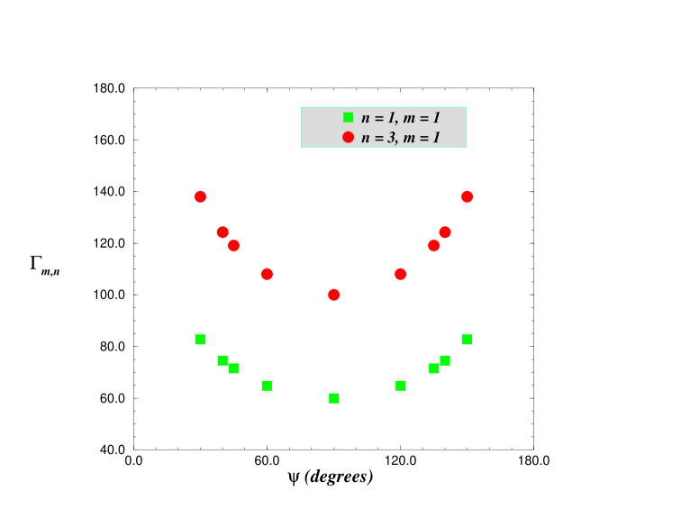
FIG. 1.: Dimensionless energy loss rate Burden loops with $(m,n)=(1,1)$ and $(1,3)$.

We plot in Fig. 1 $\Gamma_{m,n}$ as a function of the angle $\psi$, for the nominal value $f=1$ and for the two cases $(m,n)=(1,1)$, $(m,n)=(1,3)$. [As said above there is a simple scaling law for the dependence on $m$ and $n$.] If one compares this Figure with the figures published in [33], [2] (Fig. 7.6, p. 205 there) one sees that they give a roughly adequate numerical representation of energy losses to gravitational radiation if

$$f\simeq 0.8\,.$$ (182)

The fact that our present “best fit” value of the factor $f$ leads to values of $\Delta$ which are numerically comparable to $L$ (when $(m,n)=(1,1)$) rather than to a smaller fraction of $L$ should not be considered as physically incompatible with the idea of using a local approximation to back reaction. Indeed, on the other hand, the rough justification of the local approximation given in Section IV suggested $\Delta\sim\pi/\omega\sim\lambda/2$, i.e. something like $L/4$, and, on the other hand, numerical computations show that the energy lost to dilaton waves (with coupling $\alpha=1$) is smaller than that lost to gravitational waves by a factor of order 3 or so (part of which is simply due to the fact that there are two independent tensor modes against one scalar mode). Therefore, as we use $\Delta$ only as an effective parameter to model gravitational damping it is normal to end up with an increased value of $\Delta/L$.

Clearly, more work would be needed to confirm that the modified local dilaton reaction (171) can be used as a phenomenological representation of gravitational reaction. Our main purpose here was to clarify the crucial sign problems associated to gauge fields, and to give a first bit of evidence indicating that Eq. (171) deserves seriously to be considered as an interesting candidate for mimicking, in a computationally non-intensive way, the back reaction of gravitational radiation. We are aware that several important issues will need to be further studied before being able to use Eq. (171) in a network simulation. Some numerically adequate definition of $\lambda$ will have to be provided beyond a case by case definition, which in the case of long loops decorated by a regular array of kinks, as in Ref. [11], would be something like $2\lambda\sim L/N$ where $N$ is the total number of kinks. We note in this respect that a Burden loop with $m=1$ and $n\gg 1$ provides a simple model of a long, circular loop decorated by a travelling pattern of small transverse oscillations. However, the local approximation (171) cannot expected to be accurate in this case, because the radiation from purely left-moving or right-moving modes is known to be suppressed [2]. This suppression is not expected to hold in the more physical generic case where the transverse oscillations move both ways. The accuracy of the local approximation (171) should therefore be tested only in such more generic cases.

The explicit expression (171) must be rewritten in the temporal, but not necessarily conformal, worldsheet gauges used in numerical simulations, and the higher time derivatives in ${\cal F}_{\mu}$ must be eliminated by using (as is standard in electrodynamics [34] and gravitodynamics [32]) the lowest-order equations of motion. [These last two issues have already been treated in Refs. [14], [15].] Finally, we did not try to explore whether $\eta=1/2$ is the phenomenologically preferred value. To study this point one should carefully compare the effects of (171) on the weakening of cusps and kinks with the results based on the exact, non-local reaction force [11]. [The facts that the curves in Fig. 1 are flatter than the corresponding figures in [33], [2] suggest that a smaller value of $\eta$ might give a better fit.]

VI Conclusions

In this paper we studied the problem of the radiation reaction on cosmic strings caused by the emission of gravitational, dilatonic and axionic fields. We assume the absence of external fields. We use a straightforward perturbative approach and work only to first order in $G$. Our main results are the following.

• Using the results of Refs. [17], [18] for the renormalization of the string tension $\mu$, we write down the explicit form, at linear order in $G$, of the renormalized equations of motion of a string interacting with its own (linearized) gravitational, dilatonic and axionic fields. [Within our framework, we verified the on shell finiteness of the bare equations of motion, which is equivalent to their renormalizability.]

• We have extended a well-known result of Dirac by proving for general linearized fields that, in the decomposition (104) of the renormalized self-force, only the time-antisymmetric contribution ${\cal F}_{\mu}^{\rm reac}={\cal F}_{\mu}(A_{\rm reac})$, where $A_{\rm reac}(x)$ is the half-retarded minus half-advanced field, contributes, after integration over time, to the overall damping of the source. [This result had been assumed without proof in previous work on the topic.] The “reactive” self-force ${\cal F}_{\mu}^{\rm reac}$ is manifestly finite (and independent of the renormalization length scale $\Delta_{R}$), and is non-local.

• We have critically examined the proposal of Battye and Shellard [14], [15] (based on an analogy with the Abraham-Lorentz-Dirac treatment of self-interacting point charges) to approximate the non-local integral (105) entering the reactive self-force ${\cal F}_{\mu}^{\rm reac}$ by the local expression (108). For this purpose we found very convenient to use dimensional continuation, a well known technique in quantum field theory. We found that the local back reaction approximation gives antidamping for the axionic field, and a vanishing net energy-momentum loss for the gravitational one. We argued that the ultimate origin of these physically unacceptable results come from trying to apply the local back reaction approximation to gauge fields. The non-positivity of the local approximation to the damping comes from combining the modification of the field Green functions implicit in the local back reaction method, with the delicate sign compensations ensured, on shell only, by the transversality constraints of the sources of gauge fields.

• By contrast, we find that the local approximation to the dilatonic reaction force has the correct sign for describing a radiation damping. In the case of a non-gauge field such as the scalar dilaton there are no delicate sign compensations taking place, and the coarse approximation of the field Green function, implicit in the local back reaction method, can (and does) lead to physically acceptable results.

• Taking into account the known similarity between the gravitational and dilatonic radiations (e.g. [9]), we propose to use as effective substitute to the exact (non-local) gravitational radiation damping the “dilaton-like” local reaction force (171), with a suitably “redshifted” effective length $\Delta$, Eq. (173). This force is to be used in the right-hand side of the standard, flat-space conformal-world-sheet-gauge string equations of motion, with $\tau$- slicing linked, say, to the global center-of-mass frame of the string. The numerical calculations exhibited in Fig. 1 give some evidence indicating that Eq. (171) deserves seriously to be considered as an interesting candidate for phenomenologically approximating, in a computationally non-intensive way, the back reaction of gravitational radiation. [We recall that the exact, non-local approach to gravitational back reaction, defined by Eq. (104), is numerically so demanding that there is little prospect to implementing it in full string-network calculations.] More work is needed (e.g. by comparing the dynamical evolution of a representative sample of cosmic string loops under the exact renormalized self-force (104) and our proposed (171)) to confirm that our proposed substitute (171) is a phenomenologically acceptable representation of gravitational reaction (or of the combined dilatonic-gravitational reaction, as string theory suggests that the dilaton is a model-independent partner of the Einstein graviton).

It will be interesting to see what are the consequences of considering the effective reaction force, Eq. (171), in full-scale network simulations (done for several different values of $G\mu$) of gravitational radiation. Until such simulations (keeping track of the damping of small scale structure on long strings) are performed, one will not be able to give any precise prediction for the amount and spectrum of stochastic gravitational waves that the forthcoming LIGO/VIRGO network of interferometric detectors, possibly completed by cryogenic bar detectors, might observe.

A

In this Appendix we will give some details on the derivation of Eqs. (114), (116) using dimensional continuation.

A nice feature of analytic continuation is that it allows one to work “as if” many singular terms were regular. For instance, the factors $(\Omega^{2})^{(2-n)/2}$ and $(\Omega^{2})^{-n/2}$ that appear in Eqs. (112), (113) blow up on the light cone $(\Omega^{2}=0)$ when $n=4$. However, if we take the real part of $\epsilon=4-n$ large enough (even so large as corresponding to negative values for ${\rm Re}(n)$), these $\Omega$-dependent factors become finite, and actually vanishing, on the light cone. This remark allows one to deal efficiently with the $\Omega$-dependent factors appearing in Eqs. (112), (113). We are here interested in the contributions to $A_{\rm ret}(z)$ and $\partial_{\mu}\,A_{\rm ret}(z)$ coming from a small neighbourhood $z^{\prime}=z(\tau^{\prime},\sigma^{\prime})$ of $z=z(\tau,\sigma)$ on the worldsheet. Let us, for simplicity, denote $\omega\equiv\Omega^{2}$. We first remark that when $(\tau^{\prime},\sigma^{\prime})\rightarrow(\tau,\sigma)$, $\omega=-(z(\tau,\sigma)-z(\tau^{\prime},\sigma^{\prime}))^{2}$ admits an expansion in powers of $\tau^{\prime}-\tau$ and $\sigma^{\prime}-\sigma$ of the form

$$\omega=\omega_{2}+\omega_{3}+\omega_{4}+\ldots\,,$$ (A1)

with $\omega_{2}=-{\dot{z}}^{2}\,[(\tau^{\prime}-\tau)^{2}-(\sigma^{\prime}-\sigma)^{2}]$, and

$$\omega_{3}={\cal O}\,((\tau^{\prime}-\tau)^{3}+(\tau^{\prime}-\tau)^{2}\,(\sigma^{\prime}-\sigma)+(\tau^{\prime}-\tau)\,(\sigma^{\prime}-\sigma)^{2}+(\sigma^{\prime}-\sigma)^{3})\,,\ \hbox{etc}\ldots$$ (A2)

Then we can formally expand the $\Omega$-dependent factors of Eqs. (112), (113) in powers of $\tau^{\prime}-\tau$ and $\sigma^{\prime}-\sigma$ as follows

$$T\,[\omega^{\alpha}\,\theta(\omega)] = \left[\omega_{2}^{\alpha}+\alpha\,\omega_{2}^{\alpha-1}(\omega_{3}+\omega_{4}+\ldots)+\frac{\alpha(\alpha-1)}{2}\,\omega_{2}^{\alpha-2}(\omega_{3}+\ldots)^{2}+\ldots\right]\times$$ (A4)

$$\biggl{[}\theta(\omega_{2})+\delta(\omega_{2})\,(\omega_{3}+\omega_{4}+\ldots)+\delta^{\prime}(\omega_{2})\,(\omega_{3}+\ldots)^{2}+\ldots\biggl{]}\,.$$

Here and below, the symbol $T$ will be used to denote a (formal) Taylor expansion of any quantity following it. This expansion is valid (at any finite order) when ${\rm Re}(\alpha)$ is large enough, and is therefore valid (by analytic continuation) in our case where $\alpha=(2-n)/2$ or $-n/2$. A technically very useful aspect of the above expansion is that all the terms containing $\delta(\omega_{2})$ or its derivatives give vanishing contributions (because $\omega_{2}^{\alpha-k}\,\delta^{(\ell)}(\omega_{2})$ vanishes if ${\rm Re}(\alpha)$ is large enough, so that, by analytic continuation, $\omega_{2}^{\alpha-k}\,\delta^{(\ell)}(\omega_{2})=0$ for all values of $\alpha$). The net effect is that the contribution coming from a small string segment $-\frac{\Delta}{2}<(\sigma^{\prime}-\sigma)<\frac{\Delta}{2}$ around $\sigma$ (with $\Delta$ being much smaller that the local radius of curvature of the worldsheet) can be simply (and correctly) written as the following expansion:

$$[A_{\rm ret}(z)]^{\Delta} \equiv \epsilon\int_{\sigma-\Delta/2}^{\sigma+\Delta/2}d\sigma^{\prime}\int_{-\infty}^{\tau_{1}}d\tau^{\prime}\,\Sigma\,\omega^{\frac{2-n}{2}}\,\theta(\omega)$$ (A5)

$$= \epsilon\int_{\sigma-\Delta/2}^{\sigma+\Delta/2}d\sigma^{\prime}\int_{-\infty}^{\tau_{1}}d\tau^{\prime}\,T\,\left(\Sigma\,\omega^{\frac{2-n}{2}}\right)\,\theta(\omega_{2})$$ (A6)

$$= \epsilon\int_{\sigma-\Delta/2}^{\sigma+\Delta/2}d\sigma^{\prime}\int_{-\infty}^{\tau-|\Delta\sigma|}d\tau^{\prime}\,T\,\left(\Sigma\,\omega^{\frac{2-n}{2}}\right)\,.$$ (A7)

Here, we have introduced an arbitrary upper limit $\tau_{1}$, submitted only to the constraint $\tau_{\rm ret}<\tau_{1}<\tau_{\rm adv}$ (for instance $\tau_{1}$ could be $\tau$), and which replaces the missing theta function $\theta(z^{0}-z^{\prime 0})$ by selecting the retarded portion of the other theta function $\theta(\omega)$. As above, the symbol $T$ denotes a formal Taylor expansion. The expansion $T(\Sigma\,\omega^{\alpha})$ is simply obtained by multiplying the expansion (A1) of $\omega$ with that of $\Sigma(\tau^{\prime},\sigma^{\prime})$, namely

$$T\,[\Sigma(\tau^{\prime},\sigma^{\prime})]=\Sigma(\tau,\sigma)+(\tau^{\prime}-\tau)\,\dot{\Sigma}+(\sigma^{\prime}-\sigma)\,\Sigma^{\prime}+\ldots$$ (A8)

Similarly we have

$$[\partial_{\mu}\,A_{\rm ret}(z)]^{\Delta}=2\epsilon\int_{\sigma-\Delta/2}^{\sigma+\Delta/2}d\sigma^{\prime}\int_{-\infty}^{\tau-|\Delta\sigma|}d\tau^{\prime}\,T\,(\Sigma\,\Omega_{\mu}\,\omega^{-n/2})\,,$$ (A9)

as well as corresponding expressions for the advanced fields

$$[A_{\rm adv}(z)]^{\Delta} = \epsilon\int_{\sigma-\Delta/2}^{\sigma+\Delta/2}d\sigma^{\prime}\int_{\tau+|\Delta\sigma|}^{+\infty}d\tau^{\prime}\,T\,\left(\Sigma\,\omega^{\frac{2-n}{2}}\right)\,,$$ (A10)

$$[\partial_{\mu}\,A_{\rm adv}(z)]^{\Delta} = 2\epsilon\int_{\sigma-\Delta/2}^{\sigma+\Delta/2}d\sigma^{\prime}\,\int_{\tau+|\Delta\sigma|}^{+\infty}d\tau^{\prime}\,T\,\left(\Sigma\,\Omega_{\mu}\,\omega^{-n/2}\right)\,.$$ (A11)

As a check, we first computed the ultraviolet divergent contributions to $A_{\rm ret}(z)$ and $\partial_{\mu}\,A_{\rm ret}(z)$. We find

$$A_{\rm ret}(z) = -\frac{1}{\dot{z}^{2}}\,\left(\frac{2}{\epsilon}\right)\,2\,\Sigma\,,$$ (A12)

$$\partial_{\mu}A_{\rm ret}(z) = \frac{1}{(\dot{z}^{2})^{2}}\,\left(\frac{2}{\epsilon}\right)\,\left[-\Sigma\,\ddot{z}_{\mu}+\Sigma\,z_{\mu}^{\prime\prime}+4\Sigma\,z_{\mu}^{\prime}\,\left(\frac{z^{\prime}\cdot z^{\prime\prime}}{\dot{z}^{2}}\right)+4\Sigma\,\dot{z}_{\mu}\,\left(\frac{\dot{z}\cdot\ddot{z}}{\dot{z}^{2}}\right)\right.$$ (A14)

$$+\left.2\Sigma^{\prime}\,z^{\prime}_{\mu}-2\dot{\Sigma}\,\dot{z}_{\mu}\right]\,.$$

As it should, Eq. (A14) yields exactly the same divergences as we found in Sec. III by introducing a cut-off $\delta$ in the $\sigma^{\prime}$ integration in four dimensions. More precisely, Eq. (A14) coincides with Eq. (58) if we change $2/\epsilon\rightarrow\log\,1/\delta$. Let us note that, in the present approach, the renormalization scale $\Delta_{\rm R}$ would enter by being introduced as a dimension-preserving factor in the dimensionful coupling constants, like Newton’s constant $G$, say $G^{(n)}=G^{(n=4)}\,\Delta_{\rm R}^{\alpha}$.

Our main interest is to compute the “local approximations” to the reaction field

$$A_{\rm reac}(x)=\frac{1}{2}\,\left(A_{\rm ret}(x)-A_{\rm adv}(x)\right)\,,$$ (A15)

and its derivatives. Dimensional continuation gives an efficient tool for computing these. Indeed, combining the previous expansions we can write

$$A_{\rm reac}(x) = -\epsilon\,\int_{-\Delta/2}^{\Delta/2}d\sigma^{\prime}\int_{\tau+|\Delta\sigma|}^{+\infty}d\tau^{\prime}\,\theta(\Omega_{0}^{2})\,T_{(\tau^{\prime}-\tau)\,\mbox{\rm odd}}\left(\Sigma\,(\Omega^{2})^{\frac{2-n}{2}}\right)\,,$$ (A16)

$$\partial_{\mu}A_{\rm reac}(x) = -2\epsilon\,\int_{-\Delta/2}^{\Delta/2}d\sigma^{\prime}\int_{\tau+|\Delta\sigma|}^{+\infty}\,d\tau^{\prime}\,\theta(\Omega_{0}^{2})\,T_{(\tau^{\prime}-\tau)\,\mbox{\rm odd}}\left(\Sigma\,\Omega_{\mu}\,(\Omega^{2})^{-\frac{n}{2}}\right)\,,$$ (A17)

where $T_{(\tau^{\prime}-\tau)\,{\rm odd}}$ denotes the part of the Taylor expansion which is odd in $\tau^{\prime}-\tau$. Moreover, as we know in advance (and easily check) that the $\sigma^{\prime}$-integrands in Eqs. (A16) and (A17) are regular at $\sigma^{\prime}=0$, we can very simply write the result of the local approximation (108) (with a corresponding definition for $A_{\rm reac}^{\rm local}(z)$) by replacing $\sigma^{\prime}=\sigma$ in the integrands of Eqs. (A16), (A17)

$$[A_{\rm reac}(z)]^{\rm local}=-\epsilon\Delta\int_{\tau}^{+\infty}d\tau^{\prime}\,T_{(\tau^{\prime}-\tau)\,{\rm odd}}^{\sigma^{\prime}=\sigma}\,\left[\Sigma(\Omega^{2})^{\frac{2-n}{2}}\right]\,,$$ (A18)

$$[\partial_{\mu}\,A_{\rm reac}(z)]^{\rm local}=-2\epsilon\Delta\int_{\tau}^{+\infty}d\tau^{\prime}\,T_{(\tau^{\prime}-\tau)\,{\rm odd}}^{\sigma^{\prime}=\sigma}\,\left[\Sigma\,\Omega_{\mu}\,(\Omega^{2})^{-\frac{n}{2}}\right]\,.$$ (A19)

Here, $T_{(\tau^{\prime}-\tau)\,{\rm odd}}^{\sigma^{\prime}=\sigma}$ denotes the operation of replacing $\sigma^{\prime}$ by $\sigma$ and keeping only the odd terms in the remaining Taylor expansion in $\tau^{\prime}-\tau$. This simplifies very much the computation of the reactive terms (making it only a slight generalization of the well known point-particle results, as given for a general source in, e.g. [31]). Indeed, inserting the following expansions

$$\Omega_{\mu}(\tau^{\prime},\sigma) \simeq -(\tau^{\prime}-\tau)\,\dot{z}_{\mu}-\frac{1}{2}(\tau^{\prime}-\tau)^{2}\,\ddot{z}_{\mu}-\frac{1}{6}(\tau^{\prime}-\tau)^{3}\,{\buildrel\ldots\over{z}}_{\mu}\,,$$ (A20)

$$\Sigma(\tau^{\prime},\sigma) \simeq \Sigma(\tau,\sigma)+(\tau^{\prime}-\tau)\,\dot{\Sigma}++\frac{1}{2}(\tau^{\prime}-\tau)^{2}\,\ddot{\Sigma}\,,$$ (A21)

$$\Omega^{2}(\tau^{\prime},\sigma) \simeq -\dot{z}^{2}\,(\tau^{\prime}-\tau)^{2}\,\left[1+{(\tau^{\prime}-\tau)}\,\left(\frac{\dot{z}\cdot\ddot{z}}{\dot{z}^{2}}\right)+\frac{1}{4}\,{(\tau^{\prime}-\tau)^{2}}\,\left(\frac{\ddot{z}\cdot\ddot{z}}{\dot{z}^{2}}\right)+\right.$$ (A23)

$$\left.\frac{1}{3}\,{(\tau^{\prime}-\tau)^{2}}\,\left(\frac{{\buildrel\ldots\over{z}}\cdot\dot{z}}{\dot{z}^{2}}\right)\right]\,,\vrule width=0.0pt,height=18.0pt,depth=15.0pt$$

in Eqs. (A18), (A19) we get our main results

$${[A_{\rm reac}(z)]}^{\rm local} = \frac{\Delta}{\dot{z}^{2}}\,\left[\dot{\Sigma}-\Sigma\,\left(\frac{\dot{z}\cdot\ddot{z}}{\dot{z}^{2}}\right)\right]\,,$$ (A24)

$${[\partial_{\mu}A_{\rm reac}(z)]}^{\rm local} = \frac{\Delta}{(\dot{z}^{2})^{2}}\,\left[\frac{1}{3}\Sigma\,{\buildrel\ldots\over{z}}_{\mu}+\dot{\Sigma}\,\ddot{z}_{\mu}+\ddot{\Sigma}\,\dot{z}_{\mu}-4\dot{\Sigma}\,\dot{z}_{\mu}\,\left(\frac{\dot{z}\cdot\ddot{z}}{\dot{z}^{2}}\right)-2\Sigma\ddot{z}_{\mu}\,\left(\frac{\dot{z}\cdot\ddot{z}}{\dot{z}^{2}}\right)\right.$$ (A26)

$$\left.-\Sigma\,\dot{z}_{\mu}\,\left(\frac{\ddot{z}\cdot\ddot{z}}{\dot{z}^{2}}\right)-\frac{4}{3}\,\Sigma\,\dot{z}_{\mu}\,\left(\frac{\dot{z}\cdot{\buildrel\ldots\over{z}}}{\dot{z}^{2}}\right)+6\Sigma\,\dot{z}_{\mu}\,\left(\frac{\dot{z}\cdot\ddot{z}}{\dot{z}^{2}}\right)^{2}\right]\,.$$

These results were also obtained (as a check) from Eqs. (A16), (A17) without using in advance the simplification of putting $\sigma^{\prime}=\sigma$ in the integrand.

We have also performed a direct check on these final expressions by comparing them to the well known point-particle case [29], [30], [31]. Indeed, we have seen above that $A_{\rm reac}^{\rm local}$ and $\partial_{\mu}A_{\rm reac}^{\rm local}$ could be thought of as being generated by the effective source $\Sigma^{\rm eff.}(\tau^{\prime},\sigma^{\prime})=\delta(\sigma^{\prime}-\sigma)\,\Delta\,\Sigma(\tau^{\prime},\sigma)$, i.e. a source along the world-line ${\cal L}_{\sigma}$, defined by $\sigma^{\prime}=\sigma$. For any given value of $\sigma$, by transforming the coordinate time $\tau^{\prime}$ into the proper time $s=\int e^{\phi/2}\,d\tau^{\prime}$ along ${\cal L}_{\sigma}$ and by renormalizing in a suitable way the source $\Delta\,\Sigma(\tau^{\prime},\sigma)\equiv e^{\phi/2}\,\tilde{S}(s)$ ( so that the stringy spacetime source $\int d^{2}\sigma^{\prime}\Sigma^{\rm eff.}(\tau^{\prime},\sigma^{\prime})\,\delta^{4}(x-z(\sigma^{\prime}))$ transforms into the standard point-particle source $\int ds\,\tilde{S}(s)\,\delta^{4}(x-z(s))$), we recovered from Eqs. (A24), (A26) known point-particle results [31]. This check is powerful enough to verify the correctness of all the coefficients in Eqs. (A24), (A26).

In order to compare directly our expressions with what derived by Battye and Shellard in [14], [15], let us write Eq. (A26) for the axion field. We get

$$H^{\lambda\mu\nu}=\frac{4G\,\lambda\,\Delta}{(\dot{z}^{2})^{2}}\,\left[\frac{1}{3}\,{\buildrel\ldots\over{z}}^{\left[\lambda\right.}\,V^{\left.\mu\nu\right]}+\ddot{z}^{\left[\lambda\right.}\,\dot{V}^{\left.\mu\nu\right]}+\dot{z}^{\left[\lambda\right.}\,\ddot{V}^{\left.\mu\nu\right]}-4\dot{z}^{\left[\lambda\right.}\,\dot{V}^{\left.\mu\nu\right]}\,\left(\frac{\dot{z}\cdot\ddot{z}}{\dot{z}^{2}}\right)-2\ddot{z}^{\left[\lambda\right.}\,{V}^{\left.\mu\nu\right]}\,\left(\frac{\dot{z}\cdot\ddot{z}}{\dot{z}^{2}}\right)\right]\,,$$ (A27)

where $K^{[\lambda\mu\nu]}=K^{\lambda\mu\nu}+K^{\mu\nu\lambda}+K^{\nu\lambda\mu}$. Note that, when identifying the basic contravariant tensors $z^{\mu}$ and $V^{\mu\nu}$, the tensor $H^{\lambda\mu\nu}$ (and the force density ${\cal F}^{\mu}$) must be identical in our conventions and in the ones of Refs. [14], [15] (who use the opposite signature). However, our result Eq. (A27) differs, after the substitution $G\lambda\rightarrow f_{a}/8$, in many terms from the second Eq. (31) of Ref. [15]. Whatever be the corrections we could think of doing on the second term in their Eq. (31) (which is dimensionally wrong, probably by a copying error leading to a forgotten overdot on one of the two terms), we saw no way of reconciling their result with ours (even after expanding explicitly $V^{\mu\nu}=\dot{z}^{\mu}\,{z}^{\nu\prime}-\dot{z}^{\nu}\,{z}^{\mu\prime}$).

REFERENCES

- [1] M. Hindmarsh and T.W.B. Kibble, Rept. Prog. Phys. 58 (1995) 477.
- [2] A. Vilenkin and E.P.S. Shellard, Cosmic Strings and other Topological Defects, Cambridge University Press, Cambridge, 1994.
- [3] Y.B. Zel’dovich, Mon. Not. R. Astron. Soc. 192 (1980) 663.
- [4] A. Vilenkin, Phys. Rev. Lett. 46 (1980) 1169.
- [5] A. Vilenkin, Phys. Lett. B117 (1981) 47.
- [6] R.L. Davis, Phys. Rev. D32 (1985) 3172.
- [7] R.L. Davis, Phys. Lett. B180 (1986) 225.
- [8] R.L. Davis and E.P.S. Shellard, Nucl. Phys. B324 (1989) 167.
- [9] T. Damour and A. Vilenkin, Phys. Rev. Lett. 78 (1997) 2288
- [10] D.P. Bennett and F.R. Bouchet, Phys. Rev. Lett. 60 (1988) 257.
- [11] J.M. Quashnock and D.N. Spergel, Phys. Rev. D42 (1990) 2505.
- [12] B. Allen and R.R. Caldwell, Phys. Rev. D43 (1991) 2457.
- [13] D. Austin, E. Copeland and T.W.B. Kibble Phys. Rev. D48 (1993) 5594.
- [14] R.A. Battye and E.P.S. Shellard, Phys. Rev. Lett. 75 (1995) 4354.
- [15] R.A. Battye and E.P.S. Shellard, Phys. Rev. D53 (1996) 1811.
- [16] P.A.M. Dirac, Proc. Roy. Soc. A 167 (1938) 148.
- [17] B. Carter and R. Battye, Phys. Lett. B430 (1998) 49.
- [18] A. Buonanno and T. Damour, Phys. Lett. B432 (1998) 51.
- [19] T. Damour and G. Esposito-Farèse, Class. Quant. Grav. 9 (1992) 2093.
- [20] R. Battye and B. Carter, Phys. Lett. B357 (1995) 29.
- [21] T. Damour, in 300 Years of Gravitation, ed. by S.W. Hawking and W. Israel, Cambridge University Press, Cambridge, 1987, pp. 128–198.
- [22] F. Lund and T. Regge, Phys. Rev. 14 (1976) 1524.
- [23] A. Dabholkar and J.M. Quashnock, Nucl. Phys. B333 (1990) 815.
- [24] E. Copeland, D. Haws and M. Hindmarsh, Phys. Rev. D42 (1990) 727.
- [25] B. Carter, Phys. Lett. B404 (1997) 246.
- [26] B. Carter, Phys. Lett. B228 (1989) 466; Phys. Rev. D48 (1993) 4835.
- [27] J. Hadamard, Le problème de Cauchy et les équations aux dérivées partielles linéaires hyperboliques, Hermann, Paris, 1932; L. Schwartz, Théorie des distributions, Hermann, Paris, 1978, p. 38.
- [28] M. Riesz, Acta Mathematica 81 (1949) 1.
- [29] N.E. Fremberg, Proc. Roy. Soc. A 188 (1946) 18.
- [30] S.T. Ma, Phys. Rev. 71 (1947) 787.
- [31] T. Damour, Nuovo Cimento 26B (1975) 157.
- [32] T. Damour, in Gravitational Radiation , ed. by N. Deruelle and T. Piran, North-Holland, Amsterdam, 1983, pp. 59–144.
- [33] C.J. Burden, Phys. Lett. B164 (1985) 277.
- [34] L.D. Landau and E.M. Lifshitz, The Classical Theory of Fields, Pergamon Press, Oxford, 1962.