Lensing and caustic effects
on cosmological distances.

Abstract

We consider the changes which occur in cosmological distances due to the combined effects of some null geodesics passing through low-density regions while others pass through lensing-induced caustics. This combination of effects increases observed areas corresponding to a given solid angle even when averaged over large angular scales, through the additive effect of increases on all scales, but particularly on micro-angular scales; however angular sizes will not be significantly effected on large angular scales (when caustics occur, area distances and angular-diameter distances no longer coincide). We compare our results with other works on lensing, which claim there is no such effect, and explain why the effect will indeed occur in the (realistic) situation where caustics due to lensing are significant. Whether or not the effect is significant for number counts depends on the associated angular scales and on the distribution of inhomogeneities in the universe. It could also possibly affect the spectrum of CBR anisotropies on small angular scales, indeed caustics can induce a non-Gaussian signature into the CMB at small scales and lead to stronger mixing of anisotropies than occurs in weak lensing.

Subject headings:
cosmology - gravitational lensing  - cosmic microwave background

1 Introduction

Cosmological angular - diameter distance and ‘observer area distance’ (the latter equivalent up to redshift factors to the luminosity distance, see [1, 2]) lie at the heart of observational cosmology. They are used respectively to convert observed angles to length scales and observed solid angles to areas, at galactic distances and also on the surface of last scattering of the Cosmic Microwave Background radiation (CMB).

They are equal to each other in the case where the universe is represented on large scales by a Friedmann-Lemaître (FL) universe with an exactly spatially homogeneous and isotropic Robertson-Walker (RW) geometry. This geometry is obtained as some kind of large-scale average of the manifestly inhomogeneous matter distribution and geometry on smaller scales [3]. The local inhomogeneity causes distortion of bundles of light rays and so alters the angular diameter distance and area distance through the resultant gravitational lensing. Bertotti gave a power-series expansion for this effect[4] while the Dyer-Roeder formula [5, 6] can be used at any redshift for those many rays that propagate in the lower density regions between inhomogeneities. However this formula is not accurate for those ray bundles that pass very close to matter, where shearing becomes important.

The case of weak lensing, where no caustics occur, has been studied in depth in the last few years, including its effects on the CMB (e.g. [7]). Dyer and Oattes (1988) [8] included both shear and the varying Ricci term in a statistical study of lensing including caustics, and found that generic sources were demagnified, while a few sources were highly magnified. These results have been recently confirmed and extended by Holz & Wald [9] and by Hadrovic & Binney [10]. All of these studies suggest that an average source at high redshift in our universe will be demagnified due to caustics, and hence that the area distance is not FL on average. That the area distance of the volume averaged inhomogeneous universe need not be that of the underlying FL model is proven explicitly by Mustapha, Bassett, Hellaby and Ellis [14] and discussed further by Linder [15].

The usual assumption however, made explicit by Weinberg (1976) [11] and accepted by most workers in the field, see for example [12, 7] is that although the area distance will be inaccurately represented by the FL area distance formula on small angular scales due to the clumping of matter, when averaged over large enough angular scales that formula will be exactly correct, essentially due to photon conservation . It is our contention that this conclusion is wrong - areas will be different than in the corresponding FL universe both on small angular scales, and also when averaged to large angular scales. The increase occurs because if paths pass through underdensities (where the Dyer-Roeder approximation holds), they diverge more than in FL models; while if they pass close to matter, this will cause convergence which will often lead to caustics and an associated divergence of geodesics, again resulting in an increase of area relative to FL models shortly after the formation of the caustic. This is essentially a consequence of the non-commutativity of smoothing the geometry and calculating null geodesics , or equivalently of fitting a FL background model and determining geodesics.

This paper explains the overall nature of the effect, giving geometric arguments as to why the combined effects will not average out to give the area distance associated with the underlying matter averaged FL model. We then explain why the previous arguments either are incorrect, or do not apply to the real lumpy universe, once one follows light rays for long enough that caustics have formed in our past light cone (which is a case of considerable observational interest). We then give simple arguments as to how large the effect might be on different angular scales. While the effect associated with any single lensing object is very small, there are a very large number of objects in the sky that will cause lensing by the time our past light cone has reached the surface of last scattering. The result of all the cumulative lensing on many scales is that the past light cone will have a fractal-like structure there. Thus caustics of many scales will occur in all directions in the sky and the cumulative effect on areas can be significant.

The associated observational effects are complex, and depend on the model of matter distribution used and the angular scales observed. On small angular scales, the distance covered on the last scattering surface for a given apparent angle in a lumpy universe will generically be more than in the corresponding FL universe model (which is normally assumed as giving the correct geometry), thus ‘shrinking’ of images will occur - the apparent angular size of a given object will be smaller than expected if lensing is not taken into account, which will also affect number counts on those scales. However due to the folding over of the light cone on itself associated with caustics, on larger angular scales the effect on angular sizes will average out - the observed angular sizes of large scale structures will be little affected, even though the associated areas can be quite different, because the light rays are little deflected when considered on these scales; thus area distances and angular diameter distances will no longer be equivalent on these scales. This is consistent because the caustics cause the light cone to fold in on itself. Thus the resulting effect on particular observational relations will depend on whether it is overall angular size, or the associated observed areas, that is significant for the observations, as well as on the angular sizes of averagings implied in the observations and resulting selection effects. Detailed calculation will be required to determine the magnitude of the effect in specific cases.

The effect is demonstrated explicitly by examples in paper II [16], and the principle at the heart of the effect is confirmed in an interesting rigorous way by analysis of exact axi-symmetric models in [14]. Together they show that photon conservation does not imply that the areas corresponding to a particular solid angle will be the same as those in the background FL geometry, as claimed in Weinberg’s paper [11].

2 Why lensing causes shrinking

In general the relation between a scale $l$ perpendicular to the line of sight at redshift $z$, and the angle $\theta$ it subtends when observed will depend on $\theta$, on the direction of observation (represented by a unit spacelike vector $\bf{n}$ orthogonal to the observer’s 4-velocity), on the orientation of the arc, $l_{\perp}$, formed by the projection of $l$ onto the celestial sphere and implicitly on the angular scale $\theta_{a}$ over which observations are averaged, as well as on the redshift $z$ of the object observed, viz:

$$l=r(z,{\bf n},\theta_{a},l_{\perp},\theta)\,\theta\;.$$ (1)

Here $r(z,{\bf n},\theta_{a},l_{\perp},\theta)$ is the angular - diameter distance in a general universe, which will be anisotropic due to the shearing effects on the ray bundle, and for small angular scales will be independent of $\theta$.

We expect that this anisotropy will tend to zero (as in the background FL model) as the averaging scale increases, making the angular - diameter distance isotropic in the limit of large averaging angle, $\theta_{a}$ [15]. Thus a fairly good approximation for large - angle (e.g. COBE) experiments is that distortion (represented by large-scale shear in the null rays) is unimportant, and this is confirmed by weak lensing studies [7]. However, this does not mean that the $r(z)$ converges to the FL distance corresponding to a given averaging of the geometry. Those paths passing through empty space between clustered matter will be less focused than in the corresponding FL geometry [5]. On the other hand, sufficiently far down the null geodesics after passing strong lensing sources, conjugate points (and associated multiple images) will occur [17]-[18]; the loci of conjugate points in space time is a caustic sheet, a two-dimensional surface to which the rays are tangent [19]. The typical behaviour of null rays near these caustics has been presented in [20] (see Figure 49); the relation to gravitational lensing is discussed inter alia in [6]. When averaged over a large angular scale, the combination of effects can lead to a change in the area-distance relation.

Consider the past light cone $C^{-}(P)$ of the space-time event ‘here and now’, denoted by $P$. As a bundle of light rays ${\cal B}(d\Omega)$ generating $C^{-}(P)$ (and subtending a solid angle $d\Omega$ at $P$) passes near a lensing mass $L$, the nearer rays are distorted in towards the central ray $\gamma_{L}$ linking $P$ to $L$. Radial ratios will change (cf. [6], figure 2.3), decreasing as light rays are bent inwards in the case of a spherically symmetric lens (cf [21], Figure 2). The areas corresponding to a specific solid angle are invariant if the shear is small in a vacuum region, because transverse ratios will change in a compensating way, but there will be a change in area if distortion is significant or if there is matter present (as follows from the null Raychaudhuri equation, see e.g. [4,7])). Thus focussing is caused when strong lensing takes place, and this can be examined by ray tracing, by use of the geodesic deviation equation, or by using the optical scalar equations. Consequently (see Figure 2 in [22], or Figure 2.3 in [6]), before cusps have formed, the area $dS$ of this nearby bundle of geodesics ${\cal B}(d\Omega)$ beyond $L$ will be less than if $L$ had not been there (i.e. in the reference background case, described by an exact FL geometry). Further out from the lens, where the density is less than in the background, the effect will be reversed: areas will be larger.

A crucial point here is that we must get the overall masses right. If we take a FL universe and add a mass concentration to represent some inhomogeneity - a star, a galaxy, a galaxy cluster, or whatever - then the new universe has greater mass than the old; so we expect the areas to be different simply because the average mass density in a volume $V$ of the perturbed model that includes both $P$ and $L$, is different from that in the background model. We need to correct the perturbed model to get back to the original mass in this volume, so that the background model is correctly chosen to fit the perturbed model [3]. Or viewed differently, this is the requirement that the perturbed universe can be obtained from the background universe by rearranging masses while keeping overall mass conserved (this is the burden of the Traschen integral constraints, [23]; when they are satisfied this is equivalent to correctly fitting the background model to the lumpy universe model, see [24]). Thus when comparing lensing in a universe with given density $\rho_{0}$ with that in the corresponding FL model, we must imbed the overdensity in an exactly compensating underdensity in order to maintain the value of $\rho_{0}$. The light rays in the outer underdense region will diverge more than in the background model, and those in the inner overdense region will converge more. The standard view [11, 6] is that these effects exactly cancel: the area in the perturbed model will be exactly the same as in the background FL model.

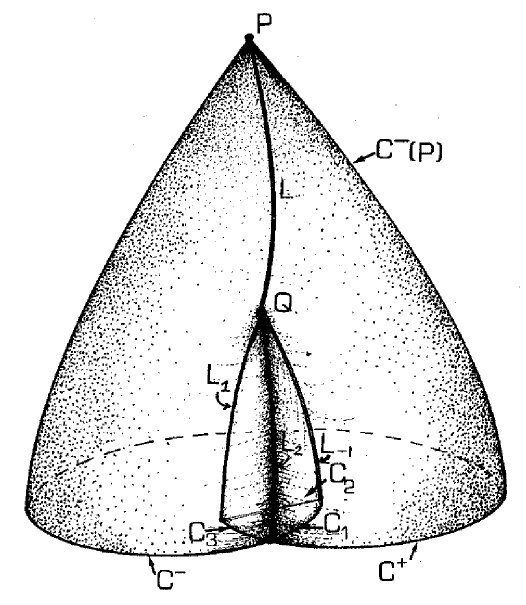
Figure 1: A lens L and resulting caustics on the past light cone $C^{-}(P)$ (2-dimensional section of the full light cone), showing in particular the cross-over line $L_{2}$ and cusp lines $L_{-1}$, $L_{1}$ meeting at the conjugate point $Q$. The intersection of the past light cone with a surface of constant time defines exterior segments $C^{-}$, $C^{+}$ of the light cone together with interior segments $C_{1}$, $C_{2}$, $C_{3}$.

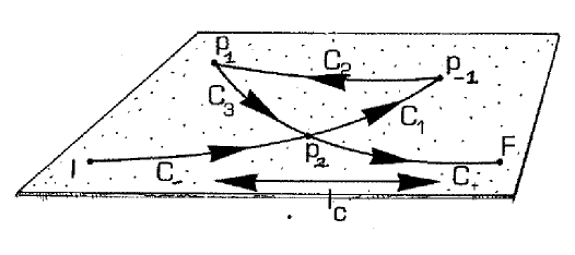
Figure 2: The imaged point moves forward along $C_{1}$ from $I$ to the cusp at $P_{-1}$, backward along $C_{2}$ to the cusp at $P_{1}$, and then forward along $C_{3}$ to $F$.

However, this does not take caustics into account. After caustics have occurred, the null rays that were converging start diverging. Indeed at a caustic an infinite convergence is instantaneously converted to an infinite divergence [25]. Thereafter, both the rays that went through the less dense regions and those that went through more dense regions and were strongly lensed are diverging more rapidly than in the corresponding exactly smooth FL model. The only rays for which the area is less are those that passed close enough to a mass to be lensed so strongly as to affect the area, but not close enough to form caustics and allow a compensating re-expansion of the null rays to occur. As most rays are subject to greater divergence (see for example the simulations by Holz & Wald [9] discussed in Section 4), on average the overall area (far enough down the light cone) will be greater than in the corresponding background model. Then on the corresponding angular scales, shrinking of images will occur. Let $r_{b}(z,\Omega_{0})$ be the area distance of the background FL universe model with a value for $\Omega$ equal to that obtained by averaging the matter distribution appropriately. Defining the pointwise shrinking factor $\gamma$ by $dl/d\theta$, then for a finite angle $\Delta\Theta$ and corresponding distance $l$,

$$l=\langle\gamma\ \rangle r_{b}\,\Delta\theta\;=\langle\gamma\rangle l_{b}\,,$$ (2)

with average angular shrinking factor $\langle\gamma(z,\theta,\phi)\rangle>1$. Correspondingly there is a change in area: pointwise

$$dS=\beta\,r^{2}_{b}\,d\Omega=\beta dS_{b}\,,$$ (3)

with average area shrinking factor $\langle\beta(z,\theta,\phi)\rangle>1$ when averaged over some solid angle $\Delta\Omega$.

As well known, there is no known covariant averaging procedure in General Relativity or agreed way of fitting a background model to the real universe [3], hence using different models for inhomogeneity and associated averaging procedures will give different estimates for $r_{b}$ (this corresponds to the gauge freedom in fitting a background model to the real universe, cf.[26]). In paper II [16] we study lensing by local inhomogeneities which are explicitly chosen to satisfy matching conditions so that the total mass in a large sphere is the same as in the background model. In [14] we use the standard astrophysical averaging - that on constant time slices in the synchronous gauge, ensuring that the mass inside any inhomogeneous regions in this gauge is the same as in the corresponding background model. An appropriate way of doing this, with explicitly stated assumptions on the potential $\Phi$, is set out in the paper by Holz and Wald [9].

Given such a choice of fitting, we are interested in finding $\langle\gamma\rangle$, $\langle\beta\rangle$ in general, and in particular after caustics have occurred. Recent Hubble Space Telescope observations imply that virtually everything beyond a redshift of 3 is at least weakly lensed, see e.g. the Hubble Deep Field for between-cluster images [27], and many signatures of lensing are seen towards clusters, see e.g. [28]-[31]. At higher and higher redshift there will be more and more lensing. We are particularly interested in any effect this has on our past light cone by the time it has reached $\Sigma$, the surface of last scattering of the CMB, for this will influence our interpretation of the CMB data. The situation here is quite different than in relating lensing to discrete sources, for (in the instantaneous decoupling approximation) the surface of last scattering is a spacelike surface; thus we are interested in the relation of the real past light cone to a spacelike surface (in contrast to its relation to timelike lines, which is relevant in considering multiple lensing of discrete objects, see [6]). Thus the issue is, What is the area $dS$ of a bundle of geodesics ${\cal B}(d\Omega)$ generating our past light cone $C^{-}(P)$ when it intersects a spacelike surface $\Sigma$, or (almost equivalently), what is the distance $l$ traversed in this surface when one scans through an angle $\theta$? However there is an important subtlety here.

2.1 Distance traveled and distance gained

The generic shape of a 2-dimensional section of the null cone occurring when simple gravitational lensing takes place, is shown in Figure 1 . Now consider, for fixed angle $\phi$, changing the direction of view ${\bf n}$ at $P$ through an arc ${\cal A}$ in the sky as the angle of observation $\theta$ increases continuously from some arbitrary initial direction $\theta_{I}$ to a final direction $\theta_{F}$, where the corresponding light rays pass through a transparent lens $L$ centred at $\theta_{L}$ ($\theta_{I}<\theta_{L}<\theta_{F}$) , and then develop caustics before intersecting the spacelike surface $\Sigma$. As the direction at $P$ continuously increases, the corresponding image point $p(\theta)$ in $\Sigma$ will move along the image of the arc ${\cal A}$ (a 1-dimensional curve) in the (2-dimensional) intersection of $C^{-}(P)$ with $\Sigma$, resulting in a series of forward, backward, and then forward motions because for each gravitational lens the 2-dimensional light cone section far enough down has at least two cusps and a cross-over (self-intersection) in it, each of these being projections of the caustic sheet in the full-spacetime.

Consider now the motion in $\Sigma$ of $p(\theta)$ as $\theta$ steadily increases from $\theta_{I}$ to $\theta_{F}$ (Figure 1b). Starting at the initial point $p(\theta_{I})=I$ on $C_{-}$, it moves on $C_{-}$ from the left, through the cross-over point $p(\theta_{-2})=P_{-2}$ (see Figure 2), along $C_{1}$ to the cusp point $p(\theta_{-1})=P_{-1}$, then back along $C_{2}$ through the lens point $p(\theta_{L})=P_{L}$ to the cusp point $p(\theta_{1})=P_{1}$, and then forward along $C_{3}$ through the cross-over point $P_{2}=p(\theta_{2})=P_{-2}$ again and onwards on $C_{+}$ to the final point $p(\theta_{F})=F$ on $C_{+}$. Hence it effectively traverses the same spatial distance (between $P_{-1}$ and $P_{1}$ along $C_{2}$) three times. If we choose $\theta_{I}$ and $\theta_{F}$ large enough, the points $I$ and $F$ will be essentially unchanged from where they would be in the background model (these rays are essentially unchanged by the lensing mass).

It will be useful to define two distances, both for the same angular change at the observer: we distinguish distance traveled $l_{t}$ along the full path:

$$I\stackrel{{\scriptstyle C_{-}}}{{\longrightarrow}}P_{-2}\stackrel{{\scriptstyle C_{1}}}{{\longrightarrow}}P_{-1}\stackrel{{\scriptstyle C_{2}}}{{\longrightarrow}}P_{1}\stackrel{{\scriptstyle C_{3}}}{{\longrightarrow}}P_{2}\stackrel{{\scriptstyle C_{+}}}{{\longrightarrow}}F\,,$$

calculated as a line integral along that path, and distance gained $l_{g}$ - how far the image point has moved in space from its starting point, calculated by determining the shortest distance between $I$ and $F$. This will be almost the same as the distance traveled along the path above but omitting all the closed loop segments, i.e it is well approximated by the line integral:

$$I\stackrel{{\scriptstyle C_{-}}}{{\longrightarrow}}P_{-2}=P_{2}\stackrel{{\scriptstyle C_{+}}}{{\longrightarrow}}F\,.$$

The difference is essentially that which occurs in a random walk - compare distance traveled by the agent (how far has his legs carried him) as against the distance moved (how far he is from where he started off). Both distances depend on the angle $\theta$, but the first increases monotonically with $\theta$, while, for each angular scale on which cusps occur, the second has a saw-tooth effect imposed on top of this uniformly increasing tendency. Because of this, the first increases with $\theta$ on average much more than the second. For large enough angles, the second will be almost the same as in the background model (because the angular positions of $I$ and $F$ will be unchanged by the lens); the backward travel due to cusps will almost exactly compensate for the extra forward travel they cause. Thus (in the case of a single lens) for large angular scales the distance gained will be almost the same as in the background; consequently (this distance being different from distance traveled), this will not be true for the distance traveled.

2.2 Addition of Areas

What this shows is that after caustics have occurred, area distances and angular size distances are different. The former corresponds broadly to distance traveled, the latter to distance gained. A strongly-lensing object $L$ will cause caustic lines on $\Sigma$, defined as the intersection of the caustic sheet with $\Sigma$. These will be spherically symmetric if the lensing object is spherically symmetric, and will be centered on the null geodesic $\gamma_{L}$ from $P$ through $L$ to $\Sigma$; similarly the critical curves (the images in the lens plane of the caustic lines) will also be circles around $\gamma_{L}$. Considering the full two-dimensional intersection ${\cal S}$ of $C^{-}(P)$ with $\Sigma$, in the spherically symmetric lens case, it will be given by rotating the 1-dimensional picture (Figure 1) about the central geodesic $\gamma_{L}$. The result is an eggcup-shaped section of the past light cone moving in to the interior and centred on $\gamma_{L}$. Defining the cusp angle $\theta_{c}$ by

$$\theta_{c}=\theta_{1}-\theta_{L}$$ (4)

(see Figure 2b), the area $A_{c}=\pi r_{b}^{2}\theta_{c}^{2}$ is covered 3 times by any solid angle centred on $\gamma_{L}$ of angle greater than about $3\theta_{c}$, where we use the background area distance $r_{b}(z)$ to convert angles to distances. Thus the real area corresponding to an angle $3\theta_{c}$ centred on $\gamma_{L}$ is about $3A_{c}$ whereas in the background model it will be simply $A_{c}$; so the area shrinking factor $\langle\beta\rangle$ will be about $3$ for such angles. However for the corresponding angular size factor $\langle\gamma\rangle$ we will find $\langle\gamma\rangle\simeq 1$ because the lens will already have little effect at angular separation $3\theta_{c}$ from $\gamma_{L}$.

To work out the area relations properly, we need to use the determinant $J$ relating solid angles at the observer to areas in the source plane [6]. The key point here is the sign of $J$: the regions where angular travel is forward as discussed above will correspond to regions where $|J|>0$; the regions where angular travel is backwards correspond to where $|J|<0$. Thus in adding up areas, we have two options: adding up the magnitudes of areas (where we assign a +ve value to all areas, i.e. we integrate $|J|$ over the relevant solid angle) or adding up signed areas (where we assign a -ve value to areas where $|J|<0$, i.e. we integrate $J$ itself over the relevant solid angle). The former corresponds to distance gained, the latter to distance traveled.

It is the latter that is relevant to number counts, for they depend on the total area occurring irrespective of the sign of $J$, and it is this we use to define area distance in the realistic universe model, and hence to determine the area ratio $\langle\beta\rangle$. Hence in equation (3), we assume all signs are positive (i.e. we take the modulus of areas and solid angles in calculating $\langle\beta\rangle$). The claim is that when the background model is properly matched to a more realistic lumpy universe model, we will find $\langle\beta\rangle>1$ on averaging over large angular scales.

3 Response to Weinberg’s arguments

The paper by Weinberg [11] explicitly considers this averaging issue, and argues that there is no overall such shrinking effect. He gives two independent arguments as to why this is so; clearly it is necessary that we answer them here.

The first point is that Weinberg’s paper does not explicitly take into account the effects of caustics, which we are identifying as important. His first argument is by explicit calculation (based on the previous work of Gunn and Press [21]) of bending by a single finite-radius clump of matter, and of the resulting intensities. However he only allows for two ray paths from the source to the observer - whereas in the generic case there will be three such paths. To first order in $q_{0}$ (i.e. assuming $\Omega_{0}\ll 1$) he finds that the luminosity distance (estimated from the combined intensities of the two images) is the same as in the FL model. If we include the general third image we may expect a different result. Additionally the estimates used are only valid for $z\simeq 1$ ([21], p.400), and hence do not cover the large-z case we are interested in.

He then gives a second argument, based on photon conservation. This argument is correct in that it determines the average number of photons intercepted by a telescope in terms of the area of a sphere drawn about the object, and works on the basis that this number is conserved (a good approximation in the context considered). The problem is that Weinberg then assumes that the area of this sphere can be calculated from the FL area formula, whereas this is precisely the issue in question. At first glance one might think the answer is obvious because here we are dealing with the up-going future light cone from the source, rather than the down-going past light cone from us, and at late times the universe is very similar to a RW universe; but by the reciprocity theorem, these light-cones are essentially equivalent to each other. Just as the past light cone of the event ‘here and now’ will develop numerous caustics as we go further into the past, so will the future light cone of the source as we go further to the future from that source provided it is far away enough in the past (if this were not so, multiple images of the same source could not occur); and the sources we are concerned with, when dealing with the CMB, are very far away - on the surface of last scattering. Just as our past light cone develops a hierarchically structured set of caustics by the time it reaches a source $S$ on the surface of last scattering, so the future light cone of the source $S$ will have developed a complementary hierarchically structured set of caustics by the time it reaches us. The area of this future light cone at the present time therefore cannot be assumed to have the FL value; indeed this is essentially the quantity we have to calculate. Thus the argument in Weinberg’s paper does not establish the result that the averaged area distance will be the same as in a FL universe, as claimed; it effectively assumes this result, by assuming this area is equal to that in a FL model.

Indeed on reflection it becomes clear that while photon conservation leads (via the reciprocity theorem) to the important result that lensing does not affect radiation intensity, it cannot determine the cross-section area of the past null cone and hence area distances, for that is determined by the Einstein field equations (specifically, by the null Raychaudhuri equation). Given that this argument does not work in the case of strong lensing, when caustics occur, it is clear that it does not work in the case of weak lensing either. In both cases photon conservation relates measured intensities to the area of the past light cone, but cannot determine the latter, which is determined by the matter present via the gravitational field equations.

4 The real past light cone

In the real past light cone, many light rays - even if passing through galaxies - will pass through low density regions all the way back to the surface of last scattering and so will have a larger area than in a FL model; the Dyer-Roeder formula will apply to them. Many others will pass near matter clumped on different scales and may be strongly lensed; this will then result in an area increase due to the occurrence of caustics, as outlined above. The additional area (about $2A_{c}$ for a spherical lens) will be very small for any particular lens, because cusp angles are small (between $3^{\prime\prime}$ and $30^{\prime\prime}$ for realistic astrophysical objects). But the point is that the number of lensing objects is very large. Each star will cause lensing, acting as an opaque lens, as will massive planets; each sufficiently concentrated galaxy core will cause lensing, acting as a transparent lens, as will each sufficiently dense cluster of galaxies .

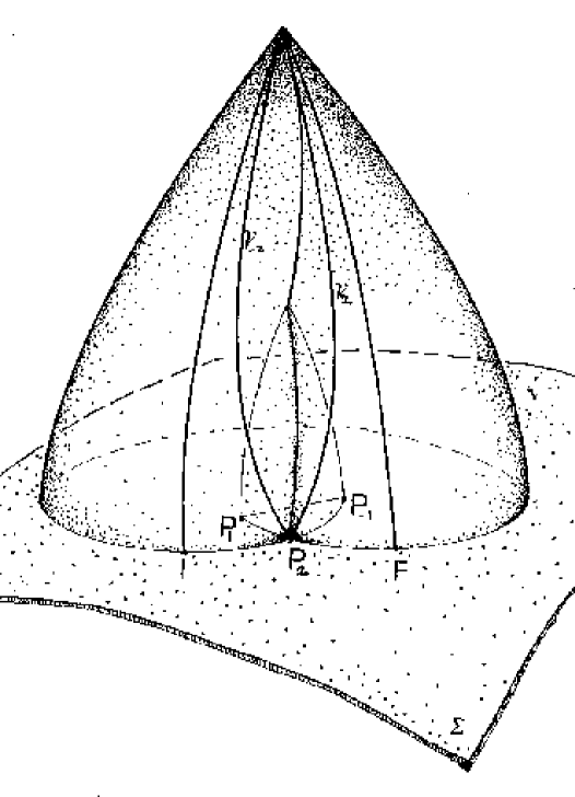
Figure 3: The unique geodesics defined by a spacelike surface $\Sigma$ intersecting the caustic structure. Geodesics $\gamma_{-2}$, $\gamma_{2}$ joining $P$ to the cross-over point $P_{2}$ and defining the cross-over angle $\theta_{2}$.

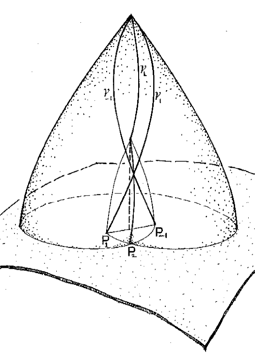
Figure 4: Geodesics $\gamma_{-1}$, $\gamma_{1}$ joining $P$ to the caustic points $P_{-1}$, $P_{1}$ and defining the cusp angle $\theta_{1}$. Also shown is the central geodesic $\gamma_{L}$.

In many cases the lensing will cause caustics to form, indeed often this will happen quite close to the lensing mass; for example in the case of the sun, bending of light by $1.75^{\prime\prime}$ at the limb will cause a caustic to occur in initially parallel light rays at that distance where the sun subtends an apparent size of $3.5^{\prime\prime}$ - which is $.0093$ parsec or $.03$ light years, and so much less than inter-stellar distances. Once a caustic occurs in our past light cone, further lensing (caused by inhomogeneities further down the past light cone) can never remove it, but can introduce new caustics. Furthermore, a single object may cause multiple caustic sheets; for example, sufficiently far down the past light cone, an elliptic lens will cause the double-caustic pattern noted by various workers [36, 19].

Hence the number of caustics in our past light cone, by any high redshift and in particular by the time it reaches the surface of last scattering, will be extremely large, of the order of at least $10^{22}$, and will occur in a hierarchically structured way with larger cusps (due to galaxies and clusters) superimposed on smaller cusps (due to stars and planets), leading to something like a fractal structure. It is important to realize that as we are interested here in effects on very distant number counts or on the CMB spatial spectrum, rather than in detailed lensing positions related to specific sources, there is no alignment problem: the surface of last scattering $\Sigma$ effectively occupies the entire sky; and most detectable objects will cause caustics by then at least on small angular scales, because $\Sigma$ is a very large distance away, corresponding to a redshift of about 1200 and most of these objects are made up of density concentrations like stars that will cause strong lensing. In addition any particular inhomogeneity may contribute to multiple cusps on different scales: multiple counting of the effects of any particular mass element is appropriate when a star causes micro-cusps and is situated in a galactic core which causes larger cusps, in a galaxy in a dense cluster which in turn causes even larger cusps. The individual stars then contribute to the formation of cusps on all these scales. Thus it is likely that an appreciable fraction of the intersection of our past light cone with $\Sigma$ will be covered by at least a single caustic.

Considering this fractured structure of the real past light cone $C^{-}(P)$ by the time it hits the surface of last scattering, it is clear there are potentially significant effects on the overall area resulting from the cumulative effects of all lenses. The overall effect will remain even after the averaging over a large angular scale due to convolution of the incoming information with a detector point spread function, because (unlike the angular distance) addition of areas is additive; the integrated magnitudes of area increments will continue accumulating as we consider larger and larger scales, although signed area increments will approximately cancel out if the model is approximately RW in the large. We argue that distance traveled (or area distance) is substantially affected when averaging on any angular scale, but that distance gained (or angular diameter distance) is significantly affected up to some angular scale $\hat{\theta}_{c}$, but not much affected on larger angular scales. The value of $\hat{\theta}_{c}$ depends on the clustering of matter at all redshifts up to the surface of last scattering; for a single spherical lens it is about $3\theta_{c}$.

4.1 Simple estimates

To estimate the relation between the various distances on the surface of last scattering $\Sigma$, we note that the rays passing through empty space or through uniformly distributed matter far enough away from inhomogeneities will correspond to the Dyer-Roeder distances. Thus the first issue here is what fraction of the sky will correspond to rays that have passed only through empty space away from clustered matter, as a function of redshift? The problem here is that there is a hierarchically structured answer to this question: the response will differ dramatically depending on the angular scale involved. For example on a microscale most light rays passing through a star cluster or galaxy pass through empty space (the cross section for collision with a star being something like $10^{-5}$ or less), whereas on the galaxy scale these rays are passing through smoothly distributed matter. Thus this fraction may be very high at small angular scales but almost zero at large angular scales.

The second issue is the effect of strong lensing. First consider the situation of a single lensing object producing a pair of cusps in the radial intersection of the light-cone with $\Sigma$. The key issue here is what is the angular size of the cusp separation at last scattering, i.e. what is the angle $\theta_{s}=\theta_{1}-\theta_{-1}$ between the two rays that reach the outer edges $P_{1}$, $P_{-1}$ of the caustic at $\Sigma$ (Figure 2a). Closely related is the angular separation $\theta_{m}=\theta_{2}-\theta_{-2}$ of the two rays that intersect $\Sigma$ in the self-intersection where the light cone folds in on itself (Figure 2b). This will be the angular separation of multiple images of a single space-time event in the surface $\Sigma$; its value will be approximately $2\theta_{s}$. Point sources, represented by timelike worldlines, move with the fundamental 4-velocity, and can be multiply imaged up to an angle $\theta_{M}\simeq(3/2)\theta_{s}$ from the centre. This maximum lensing angle can be of the order of $10^{\prime\prime}$ for nearby galaxies and $30^{\prime\prime}$ for galaxy clusters, for we have already seen deflections or arcs on these scales, but could be larger, for two lensed images in the rich cluster AC 114 are separated by $50^{\prime\prime}.6$ (see [30]) and multiple lensing may increase the effective angle significantly (see below). However many galaxies and clusters will - as coherent objects -lie below the critical surface density needed to create cusps; the stars of which they are made will nevertheless cause smaller scale cusps.

Consider then a distribution of such objects, but still only taking into account single lensing (light rays only pass close enough to one such object to be appreciably deviated). Then when we consider some angular scale $A\gg\theta_{s}$, images on those scales will be negligibly affected by the lensing. The effect is like wrinkled glass: small scale structure is blurred but large scale structure behind is reasonably clearly visible. We can immediately attain a simple estimate of the relation between the various distances mentioned above: the background distance $l_{b}$ will be well approximated by $l_{g}$ for such scales, with error at most the distance $l_{c}$ corresponding to the angular scale $\theta_{c}$, because the distances between the widely separated rays will not be affected by more than this amount. However $l_{t}$ will be different: from the argument above, for each spherical lens it will be increased by approximately 2 times the distance corresponding to $\theta_{c}$, because that path will be traversed 3 times as $\theta$ increase from $0$ to $A>3\theta_{c}$ ; the corresponding area will be triply covered, so the area will be increased by twice the area of a disk of angle $\theta_{c}$. This will occur on top of an increase of area resulting from the light rays at the lens having passed through empty space up to the time they reached the lens. For the double caustics of elliptic galaxies, there will be an increase by a factor 3 between the inner and outer caustic, and a factor 5 within the inner caustic lines.

This will be true for each single caustic line encountering the surface $\Sigma$. Thus the issue is what fraction of $\Sigma$ will be covered by single or multiple caustics? Equivalently, the effective shrinking factor will correspond to the degree of multiple covering of $\Sigma$ by caustic surfaces [8] which in turn equals the number of sources in the unperturbed direction. Defining the multiplicity of covering $M$ as the number of times the same segment of $\Sigma$ is traversed due to multiple caustics: 3 for a simple caustic as in a spherical lens and the outer region of elliptical lenses, 5 for the interior of elliptical lenses, and so on, what we are interested in is:

(a) how does $M(\theta,\phi)$ vary over a surface $\Sigma$ of constant redshift?

(b) what is its average value $\langle M\rangle$ over $\Sigma$?

(c) How does $\langle M\rangle$ vary with redshift $z$?

The value of $\langle M\rangle$ can be very high behind dense clusters of galaxies, as many caustics will overlap there; the occurrence of arcs at angular scales up to about $10^{\prime}$ confirms the multiple imaging occurring in these cases on those scales. However these clusters do not cover a large fraction of the sky; so the issue is what is its value in those areas of the sky between such galaxy clusters? What fraction of rays pass through low density areas where convergence is less than in FL models?

The increase in area due to the combination of low-density light propagation plus caustics can be significant, as is supported by recent numerical studies of strong lensing. In the extreme limit of point-mass objects, Holz & Wald [9] give results showing that for the average over all of the photon beams, $\langle\beta\rangle=1.1$ at $z=0.5$ and $\langle\beta\rangle=1.2$ at $z=2$ in an $\Omega=1,\Lambda=0$ universe while $\langle\beta\rangle=1.4$ at $z=3$ in the same model. Here $\langle\beta\rangle$ is the increase in area of the wavefront over that in the background FL model, see Eq. (3). This shows that the increase in area can be large due to the combination of rays traversing low-density regions and the existence of caustics, and is a rapidly increasing function of redshift. Their study further showed that while only $6\%$ of beams had developed caustics by $z=0.5$, $26\%$ and $37\%$ of beams had developed caustics respectively by redshifts $z=2$ and $z=3$ in the $\Omega=1,\Lambda=0$ cosmology.

These can be considered as upper limits for lensing at one scale, since they correspond to the case of point masses. The important issue then is that galaxies are made of point masses - stars - on top of the smoother dark matter halo, which itself contains a compact MACHO distribution. Thus the Holz and Wald results represent reasonable estimates for the area amplification factor due to microlensing in galaxies. What fraction of the sky is covered by galaxies? In a recent study, Premadi, Martel & Matzner [42] modeled the large scale matter distribution using a realistic P³M N-body code with extended resolution for locating galaxies, and found that all photon beams intersected a galaxy by $z=5$ if $\Omega=1,\Lambda=0$. In open or $\Lambda$-dominated cosmologies the corresponding redshift was less, of order $z\sim 3$. Intersection with each galaxy ensures caustics due to microlensing by stars adding significant area to the wavefront: between 10% in a low density universe, or 40% in a high density model. This is not removed by angular averaging, i.e. it is not important that telescopes cannot resolve individual microlensing effects for the average area distance to altered.

A number of effects alter these basic estimates. First Holz and Wald do not take their estimates out to nearly the redshift we have in mind (up to say $z=1200$). The area factor could increase greatly in this distance - say up to about 3. Secondly this only treats the micro-lensing contribution to cusps but galaxies themselves and clusters will also contribute in many cases (on larger angular scales) due to the core and/or halo densities. This effect may be somewhere from 5% to 30% increase in area. Consider for example the contribution from the cores of an isotropic population of blue galaxies with $200,000$ images per $deg^{2}$ per $mag$, giving $30$ per $arc\,min^{2}$ at $29$ mag with redshifts in the range 1 - 3. (Tyson et al [41]) A small fraction of these objects at redshifts below 2 form caustics. However, the cores of star forming regions may have masses of the order of $(1-2)\times 10^{10}M_{\odot}$ or more within a radius of $2kpc$ [39], and may substantially alter areas of light bundles that pass close to them. Galactic cores at redshift 3 or higher subtend angular diameters of $(2\,-\,3)^{\prime\prime}$, and if conditions are conducive for multiple imaging, the total (core + caustic) angle is about $(10\,-\,12)^{\prime\prime}$ (the core + cusp angle is half the caustic angle), so that the each lens has a cross-section of about $17\,-\,18$ square arcseconds. For the population of blue galaxies at $29$ mag alone, this totals to $4.6\%$ of the sky covered with caustics due to lenses between $z=1$ and $z=3$, so that the covering factor amongst the population of blue galaxies is $109.2\%$ for $\Omega=1$. At a redshift of $5$ the covering is about $115\%$; and we are interested in what happens by the time we reach the surface of last scattering.

The way we model the matter distribution is crucial. Ignoring the point-like masses in galaxies and treating only the smooth component, the effects of caustics become almost negligible, even at $z\sim 3$ [9]. In some sense this is obvious though, since spatial averaging in the limit must remove all lensing effects. However, this averaging is unphysical. In the real universe microlensing will take place in each galaxy and increase the actual area of the past light cone significantly, and on top of this we must allow for any increase due caustics caused by galaxy cores and galaxy clusters.

There is another, extremely model-dependent complication: that of the effects of multiple small-angle scattering between $P$ and $\Sigma$. When this takes place, there are two effects: firstly, this can introduce new caustics in the past light cone structure (but cannot remove any that already exist). Secondly, it will alter the angular size of existing caustics, leading to a random walk in the effective angle $\theta_{c}$ for a given lens, potentially leading to overall deflection distances that can be quite large if sufficient such scatterings take place. How large depends on the number of scatterings and angle of each one, in turn depending on the distribution of inhomogeneities all the way back to $\Sigma$, but they can potentially correspond to angles of $\sim 1^{\circ}$ [38].

It is clear then that in a realistic model of the universe, the past light cone is an extremely complex object covered with cusps on many angular scales. The probability distribution for $\theta_{c}$ will be peaked at angles from microarcseconds to at least $30^{\prime\prime}$, but may extend up to $30^{\prime}$ or so because of multiple scatterings combined with the effects of superclusters, which could be significant [40]. There will be a tail up to larger angular scales due to black holes, but of very low amplitude. We estimate an area shrinking factor, when averaged on large scales (or over the whole sky), of between 1.1 and 3, at the surface of last scattering; it could be greater.

5 Observational effects

The effect on observations could be appreciable at some angular scales once the cumulative effect of lensing has started to build up - at $z>3$ and beyond. In measurements that depend on area effects, the increase in area due to shrinking will broadly correspond to the multiplicity $M$. The actual observational effects will depend on the 2-dimensional distribution of cusps on surfaces of constant redshift such as $\Sigma$, which cannot easily be estimated from the 1-dimensional projections considered here. The figures obtained from such studies should correspond to those obtained by considering the rays propagating through low density regions only, because of the overall necessity to average out to a FL geometry on large scales.

Number counts will be altered when $\langle\beta\rangle>1$ because the areas covered by the light rays in a given solid angle are larger than estimated from the FL formula, by the area shrinking factor $\langle\beta\rangle~{}\simeq~{}\langle M\rangle$; however the detection probability will be lowered and this will tend to compensate. This is taken into account already in detailed lensing studies, but not perhaps in all high-z number count analyses where it might make a difference at the few-percent level.

The angular correlations of CMB fluctuations will also be affected by strong lensing, and is expected to cause much stronger alterations than occurs with weak lensing. However the effect is not just an alteration of apparent scale, because the distance traveled along the surface of last scattering $\Sigma$ by the measuring beam is the distance traversed $l_{t}$ (cf above), which is greater than the distance gained $l_{g}$ (the extent of each pair of cusps is traversed three times, rather than once).

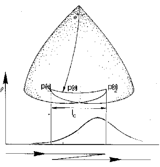
Figure 5: Sampling of an inhomogeneity by the observational point at a caustic results in a change of the observed profile, because the same region of the profile is traversed 3 times by the observational point.

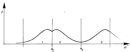
Figure 6: A Gaussian profile will not remain a Gaussian profile.

If we consider an observer sweeping a narrow beam across the sky and measuring incoming radiation in that direction, at the surface of last scattering this beam will traverse the cusps that occur in the intersection of the past light cone with the surface of last scattering, consequently moving forward, backward, and then forward each time such a cusp occurs [see Section 2 above] and almost performing a random walk when one takes into account the whole hierarchical structure of these cusps. Thus any particular small-scale temperature fluctuation will be sampled several times as it is scanned both forwards and backwards by the measuring beam; hence any Gaussian fluctuations on these scales will be measured as non-Gaussian on these scales; in effect, the actual spatial distribution is convolved with the saw-tooth sampling pattern. This will induce non-Gaussianities in the CMB anisotropies at the scales of the largest caustics [Figure 3].

What is measured on large scales is determined by the distance gained $l_{g}$, which tells us when the sampling point reaches new large-scale features of the inhomogeneous distribution of matter on the last scattering surface. The smaller backward and forward traverses are then averaged over in an effective coarse-graining. The corresponding shrinking factor relative to the background will be significantly different from unity on scales smaller than the peak in the distribution of $\theta_{c}$ over the sky, but will be close to unity on scales rather larger this scale. To determine this distribution requires detailed modeling.

6 Conclusions

In this paper we have asked the question of how strong lensing with multiple caustics due to inhomogeneity will change cosmological distance estimators and the total area of the past null cone. This is much more complex than the case of weak lensing since it involves both nonlinearities in the matter distribution and non-perturbative, singular developments in the past null cone (even if the light-bending is weak in the sense that only small-angle scattering occurs).

We find that the angular-diameter distance is not strongly affected on large angles but that the all-sky averaged area distance is significantly increased due to the folding of the null cone after multiple caustic formation. The fact that photon conservation does not forbid this has been explained, and an explicit, very detailed example of the basic underlying effect is presented in [14]. Paper II [16] shows explicitly how ‘shrinking’ (the increase in the area distance) occurs for compensated spherical lenses. These conclusions are supported by other studies, e.g. [8, 9], showing that most sources are demagnified rather than amplified when lensing occurs and caustics are taken into account.

The increase of total wavefront area at high redshift ($z>3$) is, however, strongly dependent on the model of the matter distribution used. Spatial averaging of nonlinearities, or the use of smoothed, linear matter distributions, may have a relatively mild effect on weak lensing [7], but is known to strongly affect caustic formation and wavefront areas [9]. The critical issue underlying the effect we point out here, is that one is not allowed to smooth the matter distribution before calculating the null geodesics, because in the limit this excludes caustics. This explains the difference in results between the weak lensing and Swiss-Cheese or semi-Swiss-Cheese [9] calculations. Our results are hence in accord with those found in the Swiss-Cheese type models .

Caustics are expected to alter significantly observations of the CMB on small angular scales: principally they induce a non-Gaussian signature in the temperature anisotropies at the scale corresponding to the peak in the caustic distribution function . They will induce stronger changes to the angular correlation function and hence the $C_{\ell}$ of the anisotropies than does weak lensing, simply because they involve non-perturbative mixing effects. It is just conceivable they could affect the spectrum at $\ell<200$ due to multiple scatterings. If their effects do reach this far, caustics will alter the primary and secondary Doppler peaks, thereby contaminating parameter estimation programs [37].

In a previous draft of this paper, we suggested that the Dyer Roeder distance might be usable on larger angular scales than generally supposed. This was criticized [7] on the grounds of photon conservation and neglect of shear. Here we propose an alternative interpretation of the Dyer Roeder distance - namely that it can be used to approximate the average area distance, including the shrinking due to caustics, after all-sky averaging has been performed (thus giving it a validity in the opposite regime to its normal implementation). This is based on the assumption that caustics will be distributed in a statistically isotropic manner consistent with the symmetries of the matter correlation function. The Dyer Roeder $\alpha$ parameter thereby becomes related to the probability distribution of caustics and hence again back to the degree of inhomogeneity in the universe.

In any case the main conclusion of the paper is that one should not assume the area-averaging result holds on large angular scales; rather the way angles relate to areas, and the consequent effect on observations, should be explicitly calculated for specific matter distributions. This paper and its companions show conclusively that the effect can occur. How significant it is depends on the detailed matter distribution; it will probably be small in most practical applications, but there might be circumstances where it is interesting.

Acknowledgments

The authors would like to thank Igor Barashenkov and Marco Bruni for help at critical stages of writing. They would also like to thank Jurgen Ehlers, Uro$\breve{s}$ Seljak, Malcolm MacCallum, and Nazeem Mustapha for comments on earlier drafts, and the Caltech and Cambridge (UK) lensing groups for comments that led us to more realistic estimates of the effect than suggested in earlier drafts. BAB would like to thank Jeffrey Cloete for enlightening discussions over the years. We thank the FRD (South Africa) for financial support, and Mauro Carfora for drawing most of the diagrams.

References

- [1] G. F. R. Ellis, Relativistic Cosmology, Proc. of the Int. School of Physics “Enrico Fermi”, ed R. K. Sachs, (New York: Academic Press), (1971).
- [2] S. Weinberg, Gravitation and Cosmology, (Wiley and Sons:New York, 1973).
- [3] G. F. R. Ellis and W. R. Stoeger, Classical Quant. Grav. 4, 1697 (1987).
- [4] B. Bertotti, Proc. Roy. Soc. Lond. A294, 195 (1966).
- [5] C. C. Dyer and R. C. Roeder, Ap. J. Lett. 180, L31 (1973).
- [6] P. Schneider, J. Ehlers and E. E. Falco Gravitational Lenses, (Springer-Verlag, Berlin, 1992).
- [7] U. Seljak, Ap. J, 463, 1 (1996).
- [8] C. C. Dyer and L. M. Oattes, Astrophys J. 326, 50 (1988).
- [9] D. E. Holz & R. M. Wald, astro-ph/9708036 (1997)
- [10] F. Hadrovic & J. Binney, astro-ph/9708110 (1997)
- [11] S. Weinberg, Astrophys J, 208, L1, (1976).
- [12] J. Ehlers and P. Schneider, Astron Astrophys 168, 57 (1986).
- [13] G. F. R. Ellis, in General Relativity and Gravitation, Ed. B. Bertotti et al (Reidel, 1984), 215-288.
- [14] N. Mustapha, B. A. Bassett, C. W. Hellaby and G. F. R. Ellis. Paper II, submitted to Class Quant Grav, gr-qc/9708043 (1997).
- [15] E. V. Linder, astro-ph/9801122 (1998)
- [16] D. Solomans and G. F. R. Ellis. Paper III, submitted to Class Quant Grav, (1998).
- [17] S. Seitz and P. Schneider, Max-Planck-Institut Prepritn MPA 775; (1993).
- [18] W. Hasse, M. Kriele, and V. Perlick. Class Quant Grav 13, 1161 (1996).
- [19] R. D. Blandford and R. Narayan, Ann Rev Ast Ast 30, 311 (1992).
- [20] R. Penrose. Techniques of Differential Topology In Relativity. Society for Industrial and Applied Maths (Philadelphia, 1972).
- [21] W. H. Press and J. E. Gunn, Astrophys J 185, 397 (1973).
- [22] S. Refsdal, Mon Not Roy Ast Soc 128, 23 (1964).
- [23] J. Traschen, Phys Rev D 29, 1563 (1984); D31, 283 (1985).
- [24] G. F. R. Ellis and M. Jaklitsch: Astrophys. Journ. 346, 601-606 (1989).
- [25] S. Seitz, P. Schneider, and J. Ehlers, Class. Quant. Grav. 11 (1994) 2345.
- [26] G F R Ellis and M Bruni. Phys Rev D40, 1804-1818 (1989).
- [27] S. D. J. Gwyn and F. D. A. Hartwick. Astrophys Journ 468, l77 (1996).
- [28] I. Smail, R. S. Ellis and M. J. Fitchett, MNRAS 270, 245 (1994).
- [29] I. Smail, R. S. Ellis, M. J. Fitchett and A. C. Edge, MNRAS 273, 277 (1995).
- [30] I. Smail, W. J. Couch, R. S. Ellis and R. M. Sharples, Astrophys J 440, 501 (1995).
- [31] D. W. Hogg, R. Blandford, A. Kundic, C. D. Fassnacht, and S. Malhotra. Astrophys Journ 467, L73 (1996).
- [32] R. Nityanda. In Gravitational lensing, ed. Y Mellier, B Fort and G Soucail. Springer Lecture Notes in Physics Volume 360 (Springer, 1990).
- [33] B. Fort and Y. Mellier, Astron Astrophys Rev 5: 239 (1994).
- [34] S. Refsdal and J. Surdej. Rep Prog Phys 56, 117 (1994).
- [35] R. Di Stefano and A.A. Esin, Astrophys Journ 448, L1 (1995).
- [36] R. D. Blandford and R. Narayan, Astrophys Journ 310, 568 (1986).
- [37] G. Jungman, M. Kamionski, A. Kosowsky, and D.N. Spergel. Phys Rev D54, 1332 (1996).
- [38] T. Fukushige, J. Makino, and T. Ebisuzaki Astrophys J 436, L107 (1994).
- [39] Pettini et al, astro-ph/9707200 (1997).
- [40] R. Bar-Kana, Ap. J, 468, 17 (1996)
- [41] J. A. Tyson, F. Valdes, and R. A. Wenk. Astrophys Journ 349 L1 (1990).
- [42] P. Premadi, H. Martel and R. Matzner, astro-ph/9708129 (1997)