Null weak singularities in plane-symmetric spacetimes

Abstract

We construct a new class of plane-symmetric solutions possessing a curvature singularity which is null and weak, like the spacetime singularity at the Cauchy horizon of spinning (or charged) black holes. We then analyse the stability of this singularity using a rigorous non-perturbative method. We find that within the framework of (linearly-polarized) plane-symmetric spacetimes this type of null weak singularity is locally stable. Generically, the singularity is also scalar-curvature. These observations support the new picture of the null weak singularity inside spinning (or charged) black holes, which is so far established primarily on the perturbative approach.

I Introduction

The Kerr solution [1] represents the geometry of the general stationary, vacuum, spinning black hole (BH). This solution has an obvious relevance to reality, because realistic astrophysical BHs are generally spinning [2]. It is well known that a Kerr BH has a Cauchy horizon (CH) - a null hypersurface which marks the boundary of the domain of dependence for any initial hypersurface in the external world. A similar CH also exists in the Reissner-Nordstrom (RN) geometry, which describes spherically-symmetric charged BHs. The presence of a CH inside a spinning or charged BH is disturbing, because the Einstein equations do not provide a unique prediction for the extension of the geometry beyond the CH. However, it is also well known that the CH of RN and Kerr is unstable; Namely, linear perturbations of various types develop singularities at the CH, [3]–[8] suggesting that in a generic situation the smooth CH of Kerr or RN will be replaced by a curvature singularity.

For many years, the nature and exact location of this singularity were not completely clear. The prevailing point of view in the last few decades was that the spacetime singularity inside BHs is of the BKL [9] type, i.e. spacelike, oscillatory, and tidally-destructive. In the last few years, however, there is steadily growing evidence that a singularity of a completely different character forms at the CH of spinning [10, 11] and charged [12]–[15] BHs. This singularity is null [10, 12, 13, 16] rather than spacelike, and weak [10, 13] (in Tepler’s terminology [17]), rather than tidally-destructive.

So far, the most direct evidence for the formation of a null weak singularity inside generic spinning BHs stems from the nonlinear perturbation analysis of the interior Kerr geometry [10, 11]. It would obviously be important to confirm the perturbative results from alternative, non-perturbative, directions of research. Motivated by this, Yurtsever [18] suggested that plane-symmetric spacetimes could serve as an excellent test-bed for further exploring and testing the new picture of the BHs’ null weak singularity, emerging from the perturbative approach. Yurtsever based his suggestion on the following argument: If indeed a null curvature singularity exists at the CH of generic spinning (or charged) black holes, there should exist corresponding plane-wave solutions [19, 20] which admit a (locally) similar type of null singularity. Therefore, understanding the rule of such null singularities in plane-wave and colliding plane-waves (CPW) solutions [21, 22] may provide important insight into the issue of stability of the null CH singularity inside spinning (or charged) BHs.

In this paper we shall attempt to undertake this goal. We shall first construct an exact linearly-polarized (LP) ingoing plane-wave solution which admits a weak curvature singularity on a null hypersurface. Then we shall analyse the stability of this type of singularity, within the framework of (LP) plane-symmetric spacetimes, by a rigorous non-perturbative method: First we shall demonstrate the stability with respect to generic ingoing plane-wave perturbations (which preserve the plane-wave character of the solution). Then we shall introduce outgoing plane-symmetric perturbations as well, and analyse their effect on the structure of the singularity. The outgoing perturbations convert the geometry into a (LP) CPW spacetime. We shall show that the singularity remains null and weak, though curvature scalars, which were strictly zero in the original plane-wave solution, generically blow up when the outgoing perturbations turn on. (This situation is fully analogous to what is known about the black holes’ CH singularity: In a spherical charged BH, if the radiation is purely ingoing the CH singularity is non-scalar [16], but when one adds outgoing radiation, the singularity becomes scalar-curvature - the mass-inflation singularity [12]. In the case of a spinning vacuum BH, the CH singularity is scalar-curvature. [10, 23]) We conclude that the null weak singularity is locally stable within both frameworks of plane-wave solutions and CPW solutions (though the non-scalar character of the null singularity in plane-wave solutions is unstable within the framework of CPW solutions). This provides a strong support to the above-mentioned new picture of the BHs’ singularity.

In Ref. [18] Yurtsever presented a certain limiting process which maps a (local neighborhood of a) generic null singularity into a plane-wave null singularity. Based on this limiting process, Yurtsever correctly pointed out that if indeed a generic null singularity exists inside black holes, it should be asymptotically similar to a generic null singularity of a plane-wave solution. Yurtsever further argued that this plane-wave null singularity should coincide with the “singular Cauchy horizon” of the plane-wave solution. But the Killing Cauchy horizons of plane-wave solutions are known to be non-generic and unstable within the context of global initial-value problem for CPW spacetimes. [22] This led Yurtsever to the conclusion that a null singularity (e.g. inside black holes) must be locally unstable and hence unrealistic. This conclusion, we argue, is incorrect; Its derivation requires one to make two closely related assumptions:
Assumption 1: The scenario of a formation of a black hole, with a null curvature singularity inside it, from regular initial data, can be approximated in a global sense by some plane-wave (or CPW) solution with a null singularity, which evolves from regular initial data.
Assumption 2: Correspondingly, the latter null singularity should be located at the Killing Cauchy horizon of the plane-wave (or CPW) solution.
Both assumptions result from the confusion of local and global aspects of the problem. The statement that the black-hole’s null singularity is well approximated by a plane-wave null singularity holds only on a local basis. This is obvious from the nature of the limiting process described in Ref. [18], which assumes a null geodesic $\gamma$ that intersects the null singularity: It is only the “tubular” immediate neighborhood of $\gamma$ (near its intersection point with the singularity) which admits the approximate similarity to a plane-wave solutions. (See Fig. 1, in which this neighborhood is denoted by $N$.) Since the initial hypersurface of the black-hole spacetime is remote from the null singularity inside the BH, there is no way to extend $N$ up to this initial hypersurface. Therefore, despite the local similarity of the neighborhoods of the null singularities in the two spacetimes, their global features are totally different. In particular, there is no reason to relate the BH’s null singularity to the plane-wave Killing Cauchy horizon. Moreover, when considered as a simplified approximate model for the BH’s null singularity, the issue of stability of the plane-wave null singularity must be considered from the local point of view (see below), and not from the global one based on Cauchy evolution from regular initial data.

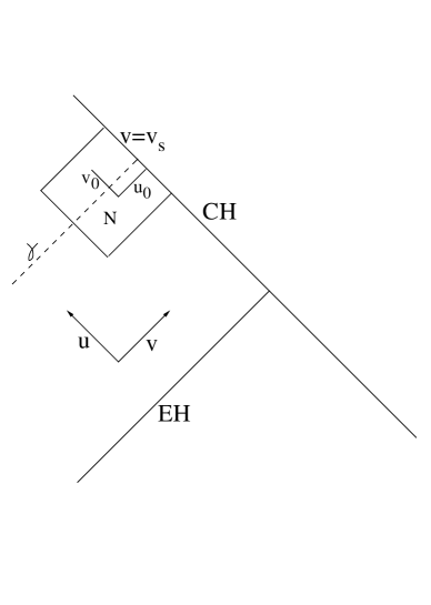
FIG. 1.: The local initial-value setup for the plane-symmetric spacetime, and its relation to the inner structure of the black hole. EH and CH are the event horizon and the singular Cauchy horizon of the black hole, respectively. The two characteristic initial null hypersurfaces, $u=u_{0}$ and $v=v_{0}$, are located in the neighborhood $N$ of the intersection point of the CH singularity and the outgoing null geodesic $\gamma$.

Our approach to the issue of local stability is based on a local (characteristic) initial-value setup. Namely, we introduce a pair of characteristic initial null hypersurfaces (denoted $u_{0}$ and $v_{0}$ in Fig. 1), both located inside the small local neighborhood $N$ of a point on the null singularity. In such an initial-value setup, the generic CPW solution depends on two freely-specifiable functions, one of the ingoing null coordinate $v$ and one of the outgoing null coordinate $u$. (In the special case of a plane-wave solution, one of these functions degenerates to a constant.) We shall first construct a specific ingoing plane-wave solution which admits a null curvature singularity at $v=v_{s}$. Then we shall add perturbations to both the above mentioned initial functions. These perturbations are generic, though bounded (and restricted in some weak sense). We shall show, by means of a non- perturbative analysis, that the null singularity at $v=v_{s}$ survives these perturbations. That is, within the framework of CPW spacetimes, the null singularity is locally stable.

In this local setup, the outgoing initial hypersurface $u_{0}$ necessarily intersects the null singularity (obviously, if we chop this hypersurface before $v=v_{s}$, the null singularity will not be included in the domain of dependence). In other words, in order to recover the null singularity, we must start with initial data at $u=u_{0}$ which are themselves singular at a certain point ($u=u_{0}$,$v=v_{s}$). [24] (This singular point will then be the “seed” of the null singularity, which will extend along the hypersurface $v=v_{s}$.) This disadvantage is unavoidable, because, as was explained above, the global plane-wave initial-value problem (starting from regular initial data) has little to do with the issue of null singularities inside black holes. In physical terms, what we show here is that a singularity (of a certain type) at the initial data generically propagates along the characteristic line and thereby produces a null singularity. This observation is not trivial: One might conceive that the nonlinearity of the field equations will generically prevent the formation of a null singularity, and a spacelike singularity will form instead (this is essentially the possibility suggested by Yurtsever [18]). Our local stability analysis shows that this is not the case: The null singularity of plane waves is locally stable within the frameworks of plane-wave and CPW spacetimes.

Recently, Ori and Flanagan (OF) [25] used another construction to demonstrate the local genericity of null weak singularities. The construction by OF is more powerful than the one presented here, as it demonstrates local (functional) genericity within the framework of the fully-generic class of vacuum solutions, without any symmetry. The present work is advantageous in certain respects, however: First, the mathematical construction by OF heavily depends on analyticity: It is restricted to analytic initial-value functions, and is primarily based on the Cauchy-Kowalewski theorem. The present construction does not make any assumptions about the analyticity of the initial functions (we only demand smoothness), and is based on the hyperbolic nature of the field equations. Second, the type of local asymptotic behavior covered by the present analysis is slightly more general than that of OF, as explained in section V. In addition, the generalization to null singularities with more realistic types of local asymptotic behavior will be much easier to implement within the present framework of CPW spacetimes (this is again a consequence of the lack of any reference to analyticity in the present method; see section V). Third, the simplicity of the CPW solutions makes the present construction more useful for investigating various features of the null singularity. We should also mention another attempt to use a local construction for investigating the BH’s null CH singularity, made earlier by Brady and Chambers [26]. Their construction, however, only addressed the constraint equations on two null hypersurfaces, and the compatibility with the six evolution equations was not considered there. In particular, the analysis in Ref. [26] does not rule out the possibility that a spacelike singularity will form immediately at the singular “point” [analogous to ($u_{0}$,$v_{s}$)] at the future edge of the outgoing initial null hypersurface. The present construction (like that of OF) takes care of the full set of vacuum Einstein equations.

Throughout this paper we restrict attention to linearly-polarized (LP) plane-wave and CPW solutions, for simplicity. We do not expect the qualitative results to be different in the more general case of arbitrarily polarized solutions. The analysis in the arbitrarily polarized case is more complicated, but still appears to be feasible.

This paper is organized as follows. In section II we shall construct an explicit ingoing LP plane-wave solution with a non-scalar parallelly-propagated (PP) null weak singularity, to which we shall refer as the basic solution. Then, in section III we shall perturb this basic solution by generic (though bounded) LP ingoing perturbations, and show that the singularity remains non-scalar, PP, null, and weak. This demonstrates that the non-scalar null weak singularity is a generic feature of (LP) plane-wave spacetimes. In section IV we shall add generic (LP) perturbations in the outgoing direction. The geometry is now described by the CPW solution. We shall show that the singularity remains null and weak, though generically the outgoing perturbations convert the non-scalar PP curvature singularity into a scalar-curvature singularity. Finally, in section V we shall discuss the extent and implications of our results.

II Basic Singular Plane-Wave Solution

The LP plane-wave spacetimes can be described by the line element

$$ds^{2}=-du\,dv+e^{-U(v)}\,\left[{e^{V(v)}dx^{2}+e^{-V(v)}dy^{2}}\right]\;.$$

The only non-trivial vacuum Einstein equation is

$$2U_{,vv}-{U_{,v}}^{2}-{V_{,v}}^{2}=0\;.$$

Since there are two non-trivial functions [$U(v)$ and $V(v)$] and one constraint, Eq. (2), plane-wave solutions are described by one arbitrary function of $v$. To simplify the calculations, we take the freely-specified function to be $U(v)$. Equation (2) then becomes an integral for $V(v)$. [When the freely-specified function is taken to be $V(v)$, Eq. (2) becomes a non-linear differential equation for $U(v)$.]

We wish to construct an explicit solution in the range $v_{0}\leq v<v_{s}$ which develops a null weak curvature singularity at $v=v_{s}$. In general, such a solution will be obtained from any function $V(v)$ which is smooth at $v_{0}\leq v<v_{s}$ and continuous at $v=v_{s}$, but with $V_{,v}$ diverging at $v=v_{s}$. We shall now construct a simple explicit solution of this type. To shorten the notation, we take $v_{s}=0$ and define

$$w\equiv|v|^{1/n}=(-v)^{1/n}\;,$$

where $n$ is any constant $>2$ . (Note that with the choice $v_{s}=0$, both $v$ and $v_{0}$ are negative.) We now take

$$U(v)=-\,(n-2)\,a^{2}w^{2}\equiv U_{0}(v)\;,$$

where $a$ is a positive dimensional constant. Solving Eq. (2), we obtain

$$V(v)=(n-2)\,\left[{aw\,\left({1-a^{2}\,w^{2}}\right)^{1/2}+\arcsin\left({aw}\right)}\right]\equiv V_{0}(v)\;.$$

(For concreteness we took here the positive root for $V_{,v}$, and set the integration constant such that $V$ vanishes at $v=0$. This causes no loss of generality: Adding a constant to $V$ or changing its sign amounts to rescaling the coordinates $x$ and $y$ or interchanging them, respectively.) In order to ensure the validity and regularity of $V(v)$ in the entire range $v_{0}\leq v<0$, we take $0<a\,<|v_{0}|^{-1/n}$, so that $0<aw<1$.

We shall refer to the explicit plane-wave solution (4,5) as the basic solution. In terms of our characteristic initial-value setup, this plane wave solution may be viewed as evolving from the initial data (4,5) at the characteristic hypersurface $u=u_{0}$, with trivial (i.e. u- independent) initial data along the other hypersurface, $v=v_{0}$.

An expansion of Eq. (5) near $v=0$ yields

$$V=2(n-2)aw+O\,(w^{3})\;.$$

For any function $F(w)$, we find

$$F_{,v}=-n^{-1}|v|^{1/n-1}f_{,w}\quad,\quad F_{,vv}=n^{-2}\left[{|v|^{2/n-2}f_{,ww}-(n-1)|v|^{1/n-2}f_{,w}}\right]\;.$$

Therefore, at $v=0$ the derivatives of $V$ and $U$ with respect to $v$ diverge:

$$V_{,v}\,\cong-\,\left[{2n^{-1}(n-2)a}\right]\;\,|v|^{1/n-1}\;\;,\;\;U_{,v}\,\propto\,v^{2/n-1}\;.$$

(This divergence has an invariant meaning, because $v$ is the affine parameter for the null geodesics of constant $x,y,u$ .) The second-order derivatives diverge even faster:

$$V_{,vv}\,\cong-\,\left[{2n^{-2}(n-1)(n-2)a}\right]\;\,|v|^{1/n-2}\;\;,\;\;U_{,vv}\,\propto\,v^{2/n-2}\;.$$

As a consequence, various components of the Riemann tensor diverge at $v=0$. For example, one finds that

$$R_{vxvx}={1\over 2}e^{V-U}\left({-V_{,vv}+U_{,v}V_{,v}}\right)\;,$$

and thus near $v=0$,

$$R_{vxvx}\cong-{1\over 2}V_{,vv}\cong n^{-2}(n-1)(n-2)a|v|^{1/n-2}\;.$$

Since all curvature scalars vanish in plane-wave spacetimes, there is no scalar-curvature singularity at $v=0$. One can easily verify, however, that parallelly-propagated (PP) components of the Riemann tensor diverge along null and timelike geodesics intersecting $v=0$. For example, along a null geodesic of constant $x,y,u,$ a convenient PP tetrad is

$$e_{x}^{\alpha}=e^{(U-V)/2}\kern 1.0pt\delta_{x}^{\alpha}\;\;,\;\;e_{y}^{\alpha}=e^{(U+V)/2}\kern 1.0pt\delta_{y}^{\alpha}\;\;,\;\;e_{u}^{\alpha}=\sqrt{2}\,\delta_{u}^{\alpha}\;\;,\;\;e_{v}^{\alpha}=\sqrt{2}\,\kern 1.0pt\delta_{v}^{\alpha}\;.$$

The PP tetrad component

$$e_{v}^{\alpha}\,e_{x}^{\beta}\,e_{v}^{\gamma}\,e_{x}^{\delta}\,R_{\alpha\beta\gamma\delta}=2e^{(U-V)}\kern 1.0ptR_{vxvx}$$

diverges like $|v|^{1/n-2}$.

Thus, there is a PP curvature singularity at $v=0$. However, because $U=V=0$ there, the line element (1) is well-define (i.e. finite and non-degenerate) even at $v=0$. It then follows that the curvature singularity at $v=0$ is weak (in Tipler s terminology [17]). We conclude that the hypersurface $v=0$ is a null, weak, PP curvature singularity. Note also that no other singularity occurs in the range $v_{0}\leq v<0$ , because $U$ and $V$ are smooth ($C^{\infty}$) functions of $w$.

III Stability To Ingoing Plane-Wave Perturbations

In this section we shall analyse the stability of the basic plane-wave solution (4,5) within the framework of (LP) plane waves. The basic solution is characterized by the initial functions $U_{0}(v)$ and $V_{0}(v)$, Eqs. (4,5). We shall now add a small (though finite) perturbation $\Delta U(v)$ to the initial function $U_{0}(v)$:

$$U(v)=U_{0}(v)+\Delta U(v)\;.$$

In terms of the characteristic initial-value setup, this amounts to perturbing the initial data at the characteristic hypersurface $u=u_{0}$, while leaving the trivial ($u$-independent) initial data at $v=v_{0}$ unchanged (apart from a trivial constant shift, to allow for continuity at the intersection point of the two initial hypersurfaces). We assume that the perturbation $\Delta U(v)$ is a smooth function of $v$ in the range $v_{0}\leq v\leq 0$. By virtue of the constraint equation (2), this perturbation of $U(v)$ will lead to a corresponding perturbation in $V(v)$, which we now analyse. We first write Eq. (2) as

$${V_{,v}}^{2}=2U_{,vv}-{U_{,v}}^{2}={V_{0,v}}^{2}+\left[{2\Delta U_{,vv}-{\Delta U_{,v}}^{2}-2U_{0,v}\Delta U_{,v}}\right]\;.$$

Converting the derivatives of $V$, $V_{0}$, and $U_{0}$ (but not of $\Delta U$) from $v$ to $w$, recalling $v_{,w}=-nw^{n-1}$, and selecting the positive root (as before), we obtain an expression of the form

$$V_{,w}=2a(n-2)\left[{1-a^{2}w^{2}+b_{1}\Delta U_{,v}\,w^{n}+({b_{2}\Delta U_{,v}}^{2}+b_{3}\Delta U_{,vv})w^{2n-2}}\right]^{1/2}\;,$$

where $b_{1}$, $b_{2}$ and $b_{3}$ are constants that depend on $a$ and $n$. In the basic solution ($\Delta U=0$), the term in brackets is strictly positive in $v_{0}\leq v\leq 0$ (recall that $|aw|<1$). Therefore, bounds $B_{1}$,$B_{2}$ (which may depend on $a$, $n$, and $v_{0}$) exist such that the term in brackets will be strictly positive in $v_{0}\leq v\leq 0$ for any $\Delta U(v)$ satisfying

$$\left|{\Delta U_{,v}}\right|<B_{1}\;\,,\;\,\left|{\Delta U_{,vv}}\right|<B_{2}$$

throughout this range. For all perturbations satisfying the inequalities (14), $V_{,w}$ is well-defined and smooth in $v_{0}\leq v\leq 0$, and so is $V(w)$.

Turning back from $w$ to $v$, we first observe that both $U(v)$ and $V(v)$ are smooth in $v_{0}\leq v<0$ (and finite at $v=0$). That is, no new singularity appears in the range $v<0$. We still need to check the effect of the perturbation on the features of the singularity at $v=0$. From Eq. (13) it is obvious that both $V_{,v}$ and $V_{,vv}$ are unaffected at the leading order in $w$, so the asymptotic behavior at $v=0$ is still correctly described by Eqs. (8,9). It then follows that PP Riemann components [with respect to the tetrad (11)] diverge just as in the basic solution, e.g.

$$e_{v}^{\alpha}\,e_{x}^{\beta}\,e_{v}^{\gamma}\,e_{x}^{\delta}\,R_{\alpha\beta\gamma\delta}=2e^{(U-V)}\kern 1.0ptR_{vxvx}\propto\;|v|^{1/n-2}\;.$$

(However, all curvature scalars vanish, as we are still dealing with a plane-wave solution.) The hypersurface $v=0$ thus remains a non-scalar PP curvature singularity. Since both $U$ and $V$ are finite at $v=0$, the singularity is weak. We conclude that the non-scalar null weak PP curvature singularity of the basic solution is stable to small (but generic) ingoing plane-wave perturbations of the type considered here.

IV Stability To Outgoing Plane-Symmetric Perturbations

Next, we check stability with respect to outgoing perturbations; namely, we shall now assume that non-trivial initial data are present also on the ingoing initial hypersurface $v=v_{0}$. The geometry is still plane-symmetric, but is no longer a plane-wave; Rather, it is described by the (LP) CPW solution. The line element is

$$ds^{2}=-e^{-M}du\,dv+e^{-U}\,\left[{e^{V}dx^{2}+e^{-V}dy^{2}}\right]\;,$$

where the functions $M,U,V$ generally depend on both $v$ and $u$. This line element and the corresponding field equations have been discussed by several authors [21, 22]; Here we shall briefly present the field equations in a form suitable for our analysis (basically the same form as in Ref. [22]). The vacuum Einstein equations include five non-trivial equations,

$$U_{,uv}-U_{,u}U_{,v}=0$$

$$V_{,uv}-{\textstyle{1\over 2}}(U_{,u}V_{,v}+V_{,u}U_{,v})=0$$

$$M_{,uv}-{\textstyle{1\over 2}}(V_{,u}V_{,v}-U_{,u}U_{,v})=0$$

and

$$2\,U_{,vv}-{U_{,v}}^{2}-{V_{,v}}^{2}+2M_{,v}U_{,v}=0$$

$$2\,U_{,uu}-{U_{,u}}^{2}-{V_{,u}}^{2}+2M_{,u}U_{,u}=0\;.$$

The evolution equations (16a-c) form a closed system of hyperbolic equations for the three unknowns $U$, $V$, and $M$. In the characteristic initial-value setup, the values of these three functions are to be specified on the two characteristic initial null hypersurfaces, $u=u_{0}$ and $v=v_{0}$ (see Fig. 2). We shall denote the initial values of $U$, $V$, and $M$ on $u=u_{0}$ by ${}^{v}U(v)$, ${}^{v}V(v)$, and ${}^{v}M(v)$, correspondingly, and those on the other null hypersurface, $v=v_{0}$ , by ${}^{u}U(u)$, ${}^{u}V(u)$, and ${}^{u}M(u)$. We shall fix the gauge by demanding

$${}^{u}M(u)=0\;\;,\;\;^{v}M(v)=0\;.$$

Any solution of the evolution equations (16a-c) will satisfy the equations (17a,b), provided that the latter equations are satisfied on the two initial null hypersurfaces. Thus, in this gauge the Einstein equations are reduced to a set of three evolution equations (16a-c), supplemented by the demand that the six initial functions ${}^{v}V(v)$, ${}^{v}U(v)$, ${}^{v}M(v)$ and ${}^{u}V(u)$, ${}^{u}U(u)$, ${}^{u}M(u)$ will satisfy Eq. (18) and the two ordinary differential equations,

$$2\,^{v}U_{,vv}-{{}^{v}U_{,v}}^{2}-{{}^{v}V_{,v}}^{2}=0$$

$$2\,^{u}U_{,uu}-{{}^{u}U_{,u}}^{2}-{{}^{u}V_{,u}}^{2}=0\;.$$

Correspondingly, a (LP) CPW spacetime is characterized by two arbitrary initial functions, ${}^{v}U(v)$ and ${}^{u}U(u)$; The two other nontrivial initial functions, ${}^{v}V(v)$ and ${}^{u}V(u)$, will be determined from Eqs. (19a,b).

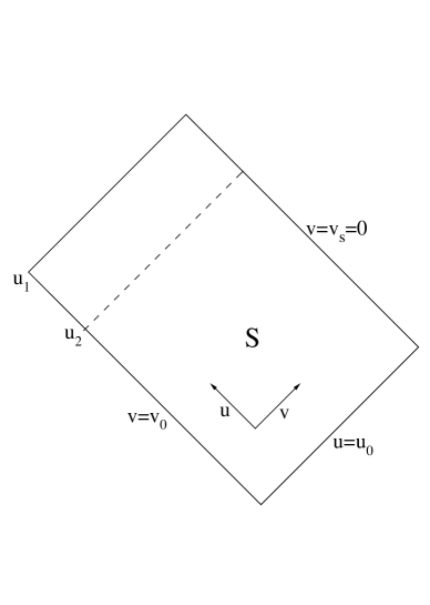
FIG. 2.: The characteristic initial-value setup for the CPW solutions constructed in Sec. IV.

In the class of CPW solutions, the ingoing plane-wave solutions form a subclass of measure zero, characterized by a trivial initial function ${}^{u}U(u)=const$. One then immediately obtains from Eq.(19b) and Eqs.(16a-c) that $U(u,v)=\kern 1.0pt{}^{v}U(v)$, $V(u,v)=\kern 1.0pt{}^{v}V(v)$, and $M(u,v)=0$, and Eqs. (1,2) are recovered. The plane-wave solutions considered in sections II and III correspond to ${}^{v}U(v)=U_{0}(v)$ and ${}^{v}U(v)=U_{0}(v)+\Delta U(v)$, respectively (and constant ${}^{u}U$). Here we shall consider nontrivial initial functions on both initial null hypersurfaces. On the outgoing hypersurface $u=u_{0}$, we take ${}^{v}U(v)=U_{0}(v)+\Delta U(v)$ as in section III. On the ingoing hypersurface $v=v_{0}$, the initial function ${}^{u}U(u)$ can be any smooth function of $u$ in the range $u_{0}\leq u\leq u_{1}$ (for some $u_{1}>u_{0}$) which satisfies the following two obvious requirements:
(i) $2\kern 1.0pt{}^{u}U_{,uu}-\kern 1.0pt{}{{}^{u}U_{,u}}^{2}>0$ in $u_{0}\leq u\leq u_{1}$; This will ensure the existence and smoothness of the function ${}^{u}V(u)$ [determined from Eq. (19b)] on the initial hypersurface $v=v_{0}$, throughout the relevant range $u_{0}\leq u\leq u_{1}$.
(ii) ${}^{u}U(u=u_{0})=\kern 1.0pt^{v}U(v=v_{0})$, which is dictated by continuity of $U(u,v)$ at the intersection point $(u_{0},v_{0})$.
Our goal is now to analyze the evolution of geometry inside the domain of dependence, $\{u_{0}\leq u\leq u_{1}\,\,,\,\,v_{0}\leq v\leq 0\}$.

We start by analyzing $U(u,v)$. Defining

$$W=e^{-U}\;,$$

Eq. (16a) is reduced to $W_{,\,uv}=0$. The solution, subject to the above initial data, is

$$W(u,v)=^{v}W(v)+^{u}W(u)-^{u}W(u_{0})\;,$$

where ${}^{u,v}W\equiv\exp(-^{u,v}U)$ and

$${}^{0}W\equiv{}^{u}W(u=u_{0})={}^{v}W(v=v_{0})\;.$$

From the smoothness of ${}^{v}U(w)$ and ${}^{u}U(u)$ it then follows that $W(u,w)$ is $C^{\infty}$ in the entire domain $u_{0}\leq u\leq u_{1}\,\,,\,\,v_{0}\leq v\leq 0$, and hence $W(u,v)$ is $C^{\infty}$ in $u_{0}\leq u\leq u_{1}\,\,,\,\,v_{0}\leq v\leq 0$ (but not at $v=0$; see below). Since $U=-\ln(W)$, the only possible singularity of $U$ at $v<0$ is at the points where $W$ vanishes. Obviously,

$$W(u=u_{0},v)=\kern 1.0pt^{v}W(v)=\exp\left[{-^{v}U(v)}\right]$$

is strictly positive at $v_{0}\leq v\leq 0$. By continuity of $W(u,w)$, there exists a constant $u_{2}$, $u_{0}<u_{2}<u_{1}$, such that $W>0$ in the entire domain $S\equiv\{u_{0}\leq u\leq u_{2}\,\,,\,\,v_{0}\leq v\leq 0\}$ (see Fig. 2). Consequently, $U(u,w)$ is smooth in $S$, and $U(u,v)$ is continuous in $S$. In addition, $U(u,v)$ is $C^{\infty}$ in the domain $S^{-}\equiv\{u_{0}\leq u\leq u_{2}\,\,,\,\,v_{0}\leq v<0\}$.

Before we analyze the evolution of $V$ and $M$ , we denote a remarkable feature of the evolution equations (16a-c): The form of these equations remain unchanged if we replace the independent variables $u$ and $v$ by new ones, $\bar{u}(u)$ and $\bar{v}(v)$ (with the unknowns $U$, $V$, and $M$ unchanged); The only modification required is to replace $\partial u$ by $\partial\bar{u}$ and $\partial v$ by $\partial\bar{v}$. We use this freedom to transform from $v$ to $w$. Consider first Eq. (16b) (with $v$ replaced by $w$). Since $U(u,w)$ is known from Eqs. (20,21), this is a hyperbolic linear equation for $V(u,w)$. Both its coefficients (i.e. $U_{,u}$ and $U_{,w}$) and its initial data [i.e. ${}^{u}V(u)$ and ${}^{v}V(w)$] are $C^{\infty}$ functions of $u$ and/or $w$. Therefore, this equation has a unique smooth solution $V(u,w)$ throughout $S$. Finally, consider Eq. (16c) for $M(u,w)$. The second term in that equation, which includes derivatives of $V$ and $U$ with respect to $u$ and $w$, is smooth in $S$, and the initial data at both initial hypersurfaces are $M=0$. Consequently, $M(u,w)$ is smooth throughout $S$.

We conclude that all three functions $U(u,w)$, $V(u,w)$, and $M(u,w)$ are $C^{\infty}$ throughout $S$ (even at $w=0$). Returning now from $w$ to the original independent variable $v$, we find that $U(u,v)$, $V(u,v)$ and $M(u,v)$ are continuous throughout $S$ and, moreover, are smooth in $S^{-}$. However, these functions will generically fail to be smooth at $v=0$. To analyse this lack of smoothness, we use Eq. (7) to evaluate the $v$-derivatives of $U$, $V$ and $M$. The maximal possible divergence rate of the first-order $v$-derivatives is $|v|^{1/n-1}$ (in fact, for $U_{,v}$ this divergence rate is never realized, because $U_{,w}$ always vanishes along the line $v=0$, but this is not important for our discussion). In addition, as long as $V_{,w}$ is nonzero at $v=0$ (which is indeed the case, as we shall immediately show), $V_{,vv}$ is dominated by the last term in the right-hand side of Eq. (7):

$$V_{,vv}\cong-\left[{n^{-2}(n-1)V_{,w}}\right]\kern 1.0pt|v|^{1/n-2}\;.$$

At $u=u_{0}$, $V_{,w}$ is nothing but ${}^{v}V_{,w}$, which is given in Eq. (13). Therefore, at $u=u_{0}$ we have

$$V_{,w}(v=0)=2a(n-2)\neq 0\quad\quad(u=u_{0})\;.$$

From the smoothness of $V(u,w)$ it then follows that

$$V_{,w}(v=0)\neq 0$$

in a neighborhood of $u=u_{0}$. In this neighborhood, $V_{,vv}$ thus diverges like $\kern 1.0pt|v|^{1/n-2}$.

The Riemann component

$$R_{vxvx}={1\over 2}e^{V-U}\left({-V_{,vv}+U_{,v}V_{,v}-M_{,v}V_{,v}}\right)$$

is dominated at $v=0$ by $V_{,vv}$:

$$R_{vxvx}\cong-{1\over 2}e^{(V-U)}V_{,vv}\cong{1\over 2}\left[{n^{-2}(n-1)e^{(V-U)}V_{,w}}\right]\,\,|v|^{1/n-2}$$

(see footnotes 1,2 above). Along an outgoing null geodesic of constant $x,y,u,$ it is convenient to use the parallelly-propagated tetrad

$$e_{x}^{\alpha}=e^{(U-V)/2}\kern 1.0pt\delta_{x}^{\alpha}\;\;,\;\;e_{y}^{\alpha}=e^{(U+V)/2}\kern 1.0pt\delta_{y}^{\alpha}\;\;,\;\;e_{u}^{\alpha}=\sqrt{2}\,\delta_{u}^{\alpha}\;\;,\;\;e_{v}^{\alpha}=\sqrt{2}\,e^{M}\kern 1.0pt\delta_{v}^{\alpha}$$

to evaluate the parallelly-propagated Riemann component

$$e_{v}^{\alpha}\,e_{x}^{\beta}\,e_{v}^{\gamma}\,e_{x}^{\delta}\,R_{\alpha\beta\gamma\delta}=2e^{(U-V+2M)}\kern 1.0ptR_{vxvx}\cong\left[{n^{-2}(n-1)e^{2M}V_{,w}}\right]\,\,|v|^{1/n-2}\;.$$

From Eq. (23) and the continuity of $M$ it is obvious that at $v=0$ the term in brackets is nonvanishing in a neighborhood of $u=u_{0}$. In this neighborhood, the parallelly-propagated Riemann component (26) diverges like $|v|^{1/n-2}$.

We find that in the perturbed spacetime, too, the hypersurface $v=0$ is a null curvature singularity. This singularity is weak, because $U$, $V$, and $M$ are all finite at $v=0$. We shall now show that this singularity is scalar-curvature. To that end, we shall calculate the scalar $K\equiv R_{\alpha\beta\gamma\delta}R^{\alpha\beta\gamma\delta}$. Although the full expression for $K$ is fairly complicated, a straightforward calculation shows that near $v=0$ it is dominated by

$$K\cong 32\,\left[{e^{2(M+U-V)}R_{vxvx}R_{uxux}+e^{2(M+U+V)}R_{vyvy}R_{uyuy}}\right]\,\;.$$

This is the only part of $K$ that includes second-order $v$-derivatives, and it diverges like $v^{1/n-2}$ (see below), whereas all other parts diverge like $v^{2/n-2}$ or slower. One can easily verify that the two terms in the brackets are equal, and that $R_{uxux}$ is of the same form as $R_{vxvx}$ [Eq. (24)], except that $v$ is replaced by $u$. Expressing the dominant part of $R_{vxvx}$ in terms of $V_{,}vv$, using Eq. (25), we obtain

$$K\cong HV_{,vv}$$

where

$$H\equiv 16\,e^{2M}\,\left({V_{,uu}-U_{,u}V_{,u}+M_{,u}V_{,u}}\right)\;.$$

In appendix A we show that for a generic choice of initial functions ${}^{u}U(u)$ and $\Delta U(v)$, $H$ is nonvanishing at $v=0$ in a neighborhood of $u=u_{0}$. In view of Eqs. (22,23), the scalar $K$ diverges there like $v^{1/n-2}$. The hypersurface $v=0$ is thus a scalar-curvature singularity.

Let us summarize the main results of this section. The perturbed spacetime (described by a CPW solution) has the following features:
i) No new singularity (spacelike or whatsoever) forms in $S^{-}$ (i.e. before $v=0$);
ii) The hypersurface $v=0$ remains a null, weak, curvature singularity;
iii) The divergence rate of the most divergent PP Riemann components is unchanged: $v^{1/n-2}$.
iv) For a generic outgoing perturbation, however, the singularity becomes scalar-curvature.

V Discussion

We have shown that within the framework of (linearly-polarized) plane-symmetric solutions the null weak singularity (4,5) is stable to both ingoing and outgoing perturbations: Both types of perturbations preserve the null weak character of the singularity. However, the outgoing perturbations generically convert the original non-scalar PP curvature singularity into a scalar-curvature singularity. This behavior is compatible with what we know about the CH singularity in black holes: In the mass-inflation model [12], outgoing radiation converts the non-scalar PP singularity of the charged Vaidya solution [16, 27] into a scalar-curvature singularity. Note also that the CH singularity in a generic spinning black hole is scalar-curvature. [10, 23]

The local stability of null weak singularities, demonstrated here (and also in Ref. [25]), provides a strong support to the new picture of the CH singularity, which was obtained primarily from the perturbative approach [10, 11]. The present model of null weak singularities in CPW spacetimes may also serve as a useful toy-model for analysing various features of null weak singularities.

Our analysis rules out the possibility that the introduction of outgoing perturbations will transform the entire null singularity into a spacelike one. It is still possible that, as the result of the outgoing perturbations, the null singularity will terminate at some $u=u_{s}>u_{0}$, where it intersects a spacelike singularity. This would be consistent with our construction, because, in the analysis in section IV, the demonstration of the regularity of $U(u,w)$ is restricted to the region $S$, i.e. $u\leq u_{2}$. It thus may be possible that a spacelike singularity will be present at $u>u_{2}$. In fact, a spacelike singularity will positively form if $W$ vanishes at some $u_{0}<u<u_{1}$, as $U=-\ln(W)$ will diverge there. (Our analysis only guarantees that this cannot happen in the neighborhood of the initial hypersurface $u=u_{0}$. Note also that if the outgoing perturbation is bounded in a suitable way, then such a divergence will be excluded in the entire range $u_{0}<u<u_{1}$.) The line $W(u,v)=0$ (when exists) is known to be the locus of a spacelike, asymptotically Kasner-like, curvature singularity [22]. Note that this situation of a null singularity becoming spacelike at a certain point also occurs in the model of a spherically-symmetric charged black hole perturbed by a self-gravitating scalar field [15]. (At present, however, it is unclear whether such a situation also occurs in vacuum spinning black holes.)

The solutions constructed here are all of the asymptotic form $V\propto v^{1/n}$ for some constant $n>2$. This is also the situation in the analysis by OF [25] - except that in the latter, unlike here, $n$ was an integer. We shall refer to this type of asymptotic behavior as the power-law asymptotic behavior. The asymptotic behavior at the CH singularity of realistic black holes (as emerges from the perturbation analyses) is somewhat different, as we now explain:
* For axially-symmetric perturbations of a Kerr BH [10] (and also for a perturbed RN BH [13]), the asymptotic behavior is $V\propto(\ln v)^{-n}$, where $n$ is the integer characterizing the power-law tails. We shall refer to it as the logarithmic asymptotic behavior.
* For nonaxially-symmetric perturbation modes of a Kerr BH, the asymptotic behavior is $V\propto(\ln|v|)^{-n}\,\cos(m\omega\;\ln|v|)$, where $\omega$ is a constant and m is the magnetic number of the mode in question. [10] We shall refer to it as the oscillatory-logarithmic asymptotic behavior.
[Here $v$ is the affine parameter along an outgoing null geodesic, with $v=0$ at the CH singularity, and $V$ stands for a typical metric function (in a suitable gauge).] One would certainly like to extend the present analysis to these more realistic types of asymptotic behavior. It seems that the generalization to the logarithmic asymptotic behavior will be almost straightforward if one replaces $w\equiv|v|^{1/n}$ of the present analysis by $w\equiv(\ln|v|)^{-n}$. The generalization to the oscillatory-logarithmic case is less straightforward, because of its non-monotonic nature. [In particular, when analysing Eq. (16b), it will not be possible to use $w\equiv(\ln|v|)^{-n}\,\cos(\omega\;\ln|v|)$ as a coordinate instead of $v$.] Still, due to the simplicity of the equations describing CPW spacetimes, hopefully the generalization to this type of asymptotic behavior will not be too difficult. Note that the approach used by OF [25] seems to be inapplicable even for the logarithmic asymptotic behavior, because it is based on analyticity: Whereas for $w\equiv(-v)^{1/n}$ (with integer $n$) $v$ is an analytic function of $w$, for $w\equiv(\ln|v|)^{-n}$ $v(w)$ fails to be analytic at $v=0$. For the same reason, in Ref. [25] the power index $n$ had to be an integer, whereas here $n$ can be any real number $>2$. In this respect, the present approach has an advantage over that of OF (however, as we mentioned in the introduction, in other respects the analysis by OF yields much more powerful results).

The present construction was restricted to $n>2$. It is straightforward, however, to extend it to any positive $n\neq 1,2$. The features of the resultant singularity at $v=0$ will significantly depend on the value of $n$. This issue deserves further investigation. It will also be interesting to generalize the present analysis to the logarithmic and oscillatory-logarithmic cases described above, and to the arbitrarily-polarized case.

Appendix A

Let us define

$$H_{0}(v)\equiv\left({V_{,uu}-U_{,u}V_{,u}+M_{,u}V_{,u}}\right)_{u=u_{0}}\;.$$

It is sufficient to show that

$$H_{0}(v=0)\neq 0\;.$$

Then, $H(u=u_{0}\,,\,v=0)=16\,e^{2M}H_{0}(v=0)$ is nonvanishing too; and from continuity $H(v=0)$ is nonzero in some neighborhood $u>u_{0}$.

In order to calculate $H_{0}(v)$ we must evolve the $u$-derivatives of $U$,$V$, and $M$ along the line $u=u_{0}$, from $v=v_{0}$ (where these derivatives are obtained directly from the $u$-dependent initial functions), and up to $v=0$. To that end we shall use the evolution equations (16a-c), which may be viewed as ordinary differential equations for the $u$-derivatives of the metric functions. Let us define

$$U_{u}(v)\equiv U_{,u}(u=u_{0},v)\;,\;V_{u}(v)\equiv V_{,u}(u=u_{0},v)\;,\;M_{u}(v)\equiv M_{,u}(u=u_{0},v)$$

and

$$V_{uu}(v)\equiv V_{,uu}(u=u_{0},v)\;,$$

so

$$H_{0}=V_{uu}-U_{u}V_{u}+M_{u}V_{u}\;.$$

From Eqs. (20,21) it follows that

$$U_{u}=\exp\left[{{}^{v}U(v)-^{0}U}\right]\,^{u}U_{,u}(u_{0})\;,$$

where ${}^{0}U\equiv{}^{v}U(v=v_{0})={}^{u}U(u=u_{0})$. For our purpose, it is sufficient to recall that the functional dependence of $U_{u}$ on the initial functions is

$$U_{u}\equiv U_{u}\left[{{}^{v}U\,;\,^{u}U_{,u}(u_{0})}\right]\;.$$

Here and below, the semicolon distinguishes between the functions of $v$ (i.e. the initial functions at $u=u_{0}$) at the left, and the parameters (obtained by evaluating the $u$-dependent initial functions, and/or their derivatives, at $u=u_{0}$) at the right. (For brevity, we omit the obvious dependence on $v$ from this list of dependencies.) Next, applying Eq. (16b) to $u=u_{0}$, we obtain

$$V_{u,v}={\textstyle{1\over 2}}(U_{u}{}^{v}V_{,v}+{}^{v}U_{,v}V_{u})\;.$$

$V_{u}(v)$ is to be determined from this ordinary differential equation, together with the initial condition $V_{u}(v=v_{0})={}^{u}V_{,u}(u_{0})$. It is straightforward to solve this linear equation explicitly (recall that $U_{u}$, ${}^{v}U$, and ${}^{v}V_{,v}$ are known), but again, for our purpose it is sufficient to recall that the functional dependence of $V_{u}$ on the initial functions is

$$V_{u}\equiv V_{u}\left[{U_{u},\,{}^{v}V_{,v},\,{}^{v}U_{,v}\,;\,^{u}V_{,u}(u_{0})}\right]\equiv V_{u}\left[{{}^{v}U\,;\,^{u}V_{,u}(u_{0}),\,^{u}U_{,u}(u_{0})}\right]\;.$$

[Here and below, we take into consideration Eq. (19a), which allows us to express ${}^{v}V_{,v}$ in terms of the function ${}^{v}U(v)$]. In a similar manner, applying Eq. (16c) to $u=u_{0}$, we obtain

$$M_{u,v}={\textstyle{1\over 2}}({}^{v}V_{,v}V_{u}-{}^{v}U_{,v}U_{u})\;.$$

$M_{u}$ can thus be obtained by a direct integration, meaning that its functional dependence is

$$M_{u}\equiv M_{u}\left[{V_{u},U_{u},\,{}^{v}V_{,v},\,{}^{v}U_{,v}\,}\right]\equiv M_{u}\left[{\,{}^{v}U\,;\,^{u}V_{,u}(u_{0}),\,^{u}U_{,u}(u_{0})}\right]$$

(recall that $M_{u}$ vanishes at $v=v_{0}$). In summary, the three functions $U_{u}$, $V_{u}$ and $M_{u}$ are fully determined from the function ${}^{v}U$ and the two parameters ${}^{u}V_{,u}(u_{0})$, ${}^{u}U_{,u}(u_{0})$.

Let us now analyse $V_{uu}$. Differentiating Eq. (16b) we find

$$V_{uu,v}\equiv\left[{(V_{,uv})_{,u}}\right]_{u=u_{0}}={1\over 2}\left({U_{,uu}V_{,v}+U_{,v}V_{,uu}+U_{,u}V_{,uv}+U_{,uv}V_{,u}}\right)_{u=u_{0}}\;.$$

Using Eq. (17b), we obtain a differential equation of the form

$$V_{uu,v}={1\over 2}{}^{v}U_{,v}V_{uu}+{1\over 2}G(v)$$

where

$$G(v)\equiv\left[\left({U_{u}}^{2}+{V_{u}}^{2}\right)/2-M_{u}U_{u}\right]\kern 1.0pt{}^{v}V_{,v}+U_{u}V_{u,v}+U_{u,v}V_{u}\;.$$

Note the functional dependence of $G(v)$,

$$G(v)=G\left[{V_{u},U_{u},M_{u},\,{}^{v}V_{,v}\,}\right]=G\left[{{}^{v}U\,;\,^{u}V_{,u}(u_{0}),\,^{u}U_{,u}(u_{0})}\right]\;.$$

Equation (A6) is a linear ordinary differential equation for $V_{uu}(v)$, whose general solution is

$$V_{uu}(v)=\exp\left({{}^{v}U/2}\right)\;\left({C+{1\over 2}\int\limits_{v_{0}}^{v}{G(v^{\prime})\exp\left[{-{}^{v}U(v^{\prime})/2}\right]dv^{\prime}}}\right)\;,$$

where $C$ is an integration constant. Recalling the initial condition,

$$V_{uu}(v=v_{0})={}^{u}V_{,uu}(u=u_{0})\;,$$

we find

$$V_{uu}(v)=Z(v)+\exp\left[{({}^{v}U-{}^{0}U)/2}\right]\,^{u}V_{,uu}(u_{0})\;,$$

where

$$Z(v)\equiv{1\over 2}\exp({}^{v}U/2)\int\limits_{v_{0}}^{v}{G(v^{\prime})\exp\left[{-{}^{v}U(v^{\prime})/2}\right]dv^{\prime}}\;,$$

namely

$$Z(v)=Z\left[{{}^{v}U\,,G}\right]=Z\left[{{}^{v}U\,;\,^{u}V_{,u}(u_{0}),\,^{u}U_{,u}(u_{0})}\right]\;.$$

Collecting Eqs. (A3,A4,A5,A7) and substituting in Eq. (A2), we can reexpress $H_{0}$ as

$$H_{0}(v)=Q(v)+\exp\left[{({}^{v}U-{}^{0}U)/2}\right]\,^{u}V_{,uu}(u_{0})\;,$$

where

$$Q(v)\equiv Z(v)-U_{u}V_{u}+M_{u}V_{u}$$

has the functional dependence

$$Q=Q\left[{{}^{v}U\,;\,^{u}V_{,u}(u_{0}),\,^{u}U_{,u}(u_{0})}\right]\;.$$

At $v=0$, we find

$$H_{0}(v=0)=q_{0}+\exp\left({\left[{{}^{v}U(v=0)-{}^{0}U}\right]/2}\right)\,^{u}V_{,uu}(u_{0})$$

where

$$q_{0}\equiv Q(v=0)=q_{0}\left[{\kern 1.0pt{}^{v}U\,;\,^{u}V_{,u}(u_{0}),\,^{u}U_{,u}(u_{0})}\right]\;.$$

We still need to express the parameters ${}^{u}V_{,u}(u_{0})$ and ${}^{u}V_{,uu}(u_{0})$ in terms of the initial function ${}^{u}U(u)$, through Eq. (19b). The latter implies

$${}^{u}V_{,u}=\pm\left({2\,^{u}U_{,uu}-{{}^{u}{U_{,u}}^{2}}}\right)^{1/2}\;\;,\;\;^{u}V_{,uu}=\pm\left({\,{}^{u}U_{,uuu}-{{}^{u}U_{,u}}\;^{u}U_{,uu}}\right)\left({2\,^{u}U_{,uu}-{{}^{u}{U_{,u}}^{2}}}\right)^{-1/2}\;,$$

so we can reexpress the functional dependence of $q_{0}$ as

$$q_{0}=q_{0}\left[{{}^{v}U\,;\,^{u}U_{,u}(u_{0}),\,^{u}U_{,uu}(u_{0})}\right]\;.$$

We can now write Eq. (A8) in the form

$$H_{0}(v=0)=h_{0}+h_{1}\,^{u}U_{,uuu}(u_{0})\;,$$

where

$$h_{0}=q_{0}\pm\exp\left[{[{}^{v}U(v=0)-{}^{0}U]/2}\right]\;\left({-{{}^{u}U_{,u}}(u_{0})^{u}U_{,uu}(u_{0})}\right)\left({2\,^{u}U_{,uu}(u_{0})-{{}^{u}U_{,u}(u_{0})^{2}}}\right)^{-1/2}$$

and

$$h_{1}=\pm\exp\left[{[{}^{v}U(v=0)-{}^{0}U]/2}\right]\,\,\left[{2\,^{u}U_{,uu}(u_{0})-\,^{u}U_{,u}(u_{0})^{2}}\right]^{\kern 1.0pt-1/2}$$

are two numbers with the same type of functional dependence:

$$h_{0,1}=h_{0,1}\left[{{}^{v}U\,;\,^{u}U_{,u}(u_{0}),\,^{u}U_{,uu}(u_{0})}\right]\;.$$

Obviously, $h_{1}\neq 0$. Therefore, in view of Eq. (A9), for any choice of initial function ${}^{v}U(v)$ and parameters ${}^{u}U_{,u}(u_{0})\,,\,^{u}U_{,uu}(u_{0})$ there only exists a single value of ${}^{u}U_{,uuu}(u_{0})$ for which $H_{0}(v=0)=0$. Thus, for a generic choice of the initial function ${}^{u}U(u)$, the inequality (A1) is satisfied.

This research was supported in part by the United States–Israel Binational Science Foundation, and by the Fund for the Promotion of Research at the Technion.

REFERENCES

- [1] R. P. Kerr, Phys. Rev. Lett. 11, 237 (1963).
- [2] J. M. Bardeen, Nature 226 64 (1970); K. S. Thorne, Astrophys. J. 191 507 (1974).
- [3] R. Penrose, in Battelle Rencontres, 1967 lectures in mathematics and physics , edited by C. M. DeWitt and J. A. Wheeler (Benjamin, New York, 1968), P. 222 .
- [4] M. Simpson and R. Penrose, Inter. J. Theor. Phys. 7 183 (1973).
- [5] Y. Gursel, V. D. Sandberg, I. D Novikov and A. A. Starobinsky, Phys. Rev. D19 , 413 (1979).
- [6] Y. Gursel, I. D Novikov, V. D. Sandberg and A. A. Starobinsky, Phys. Rev. D20 1260 (1979).
- [7] S. Chandrasekhar and J.B. Hartle, Proc. R. Soc. Lond. A 384 301 (1982).
- [8] I. D. Novikov and A. A. Starobinsky, Abstract of contributed papers of the 9th Intern. Conf. on General Relativity and Gravitation, Jena, DDR, p. 268 (1980) .
- [9] V. A. Belinsky and I. M. Khalatnikov, Zh. Eksp. & Teor. Fiz. 57, 2163 (1969) [ Sov. Phys.-JEPT 30, 1174 (1970)]; I. M. Khalatnikov and E. M. Lifshitz, Phys. Rev. Lett. 24, 76 (1970); V. A. Belinsky, I. M. Khalatnikov and E. M. Lifshitz, Usp. Fiz. Nauk. 102, 463 (1970) [Advances in Physics 19, 525 (1970)].
- [10] A. Ori, Phys. Rev. Lett. 68 , 2117 (1992).
- [11] A. Ori, Gen. Rel. Grav, 29, 881 (1997).
- [12] E. Poisson and W. Israel, Phys. Rev. D 41, 1796 (1990).
- [13] A. Ori, Phys. Rev. Lett. 67 , 789 (1991).
- [14] A. Bonano et al, Proc. Roy. Soc. A 450, 553 (1995).
- [15] P.R. Brady and J.D. Smith, Phys. Rev. Lett. 75, 1256 (1995).
- [16] W. A. Hiscock, Phys. Lett. 83A 110 (1981).
- [17] F. J. Tipler, Phys. Lett. 64A, 8 (1977).
- [18] U. Yurtsever, Class. Quantum Grav. 10 L17 (1993).
- [19] N. Rosen, Phys. Z. Sowjet. 12, 366 (1937).
- [20] R. Penrose, Rev. Mod. Phys. 37, 215 (1965).
- [21] P. Szekeres, J. Math. Phys. 13, 286 (1972).
- [22] U. Yurtsever, Phys. Rev. D 38 1706 (1988).
- [23] A. Ori, to appear in the Proceedings of the Eighth Marcel Grossmann Meeting on General Relativity, Jerusalem, Israel (1997).
- [24] This is probably the reason why the type of CPW solutions constructed here, with a locally-stable null weak singularity, was left unnoticed so far. In previous analyses of singularities in CPW spacetimes, attention was restricted to global solutions arising from regular initial data.
- [25] A. Ori, and E. E. Flanagan, Phys. Rev. D 53 R1754 (1996).
- [26] P. R. Brady and C. M. Chambers, Phys. Rev. D 51 4177 (1995).
- [27] B. Bonnor and P. C. Vaidya, Gen. Rel. Grav. 1, 127 (1970).