On the Nature of the Generic Big Bang

Abstract

Spatially homogeneous but possibly anisotropic cosmologies have two main types of singularities: (1) asymptotically velocity term dominated (AVTD)—(reversing the time direction) the universe evolves to the singularity with fixed anisotropic collapse rates ; (2) Mixmaster—the anisotropic collapse rates change in a deterministicaly chaotic way. Much less is known about spatially inhomogeneous universes. It has been claimed that a generic universe would evolve toward the singularity as a different Mixmaster universe at each spatial point. I shall discuss how to predict whether a cosmology has an AVTD or Mixmaster singularity and whether or not our numerical simulations agree with these predictions.

I Introduction

Einstein s theory of general relativity has passed all experimental tests to date and is thus, almost certainly, the classical theory of the gravitational field. Yet the universality and nonlinearity of the theory have been proven (Hawking(1970)) to imply that regular but generic initial data will (for reasonable classical matter) develop a singularity either to the future or the past. In the simplest examples, this singularity is hidden from us. The Friedmann-Robertson-Walker homogeneous, isotropic cosmology has a spacelike big bang hidden from our view by the cosmic microwave background surface of last scattering. Spherically symmetric black holes have a spacelike internal singularity hidden within an event horizon. Spatially homogeneous but anisotropic (different collapse rates in different directions) cosmologies have two types of singularities. An asymptotically velocity term dominated (AVTD) singularity means that the cosmology eventually behaves as a Kasner spacetime (fixed anisotropic expansion rates characterized by a single parameter $u$) (Isenberg and Moncrief (1990)). The other type of singularity is called Mixmaster (Belinskii et al (1971), Misner(1969)). Here the spatial scalar curvature creates a potential such that a bounce off the potential corresponds to a change of Kasner solution. The parameter $u$ changes in a deterministic way which is generally believed to be chaotic. The nature of the singularities in generic spacetimes is largely unknown. Recent analytic and numerical results demonstrate that some spatially inhomogeneous cosmologies approach a different Kasner singularity at each spatial point and thus have AVTD singularities. Belinskii, Khalatnikov, and Lifshitz (1971) (BKL) long ago conjectured that the generic singularity is locally Mixmaster-like. While this conjecture remains controversial, it provides a paradigm which can be tested.

In this talk, I shall discuss the progress toward understanding the nature of the generic cosmological singularity (Berger, Garfinkle, and Moncrief (1997)). In particular, I shall emphasize the application of a method due to Grubis̆ić and Moncrief (1993) (GM) to predict whether one should expect the singularity to be AVTD or Mixmaster-like and then discuss numerical studies to support or contradict such predictions. This work was done in collaboration with David Garfinkle (Oakland University), Vincent Moncrief (Yale University), James Isenberg (University of Oregon) and graduate students Eugene Strasser (Oakland University), Boro Grubis̆ić (Yale University), and Marsha Weaver (University of Oregon).

II Mixmaster dynamics

To understand the BKL conjecture, let us first discuss a vacuum Bianchi IX cosmology. According to the Bianchi classification of 3-dimensional homogeneous spaces, the spatial line element has the form

$$dl^{2}=A_{ij}\sigma^{i}\sigma^{j}$$ (1)

where the $A_{ij}$ are constants and the $\sigma^{i}$ s (generalizations of $dx^{i}$) satisfy

$$d\sigma^{i}=C^{i}_{jk}\,\sigma^{j}\wedge\sigma^{k}.$$ (2)

For (vacuum) Bianchi IX, $C^{i}_{jk}=\varepsilon^{i}_{jk}$, the antisymmetric symbol. The spatial dependence of the $\sigma^{i}$ s when written in a coordinate basis yield a non-vanishing spatial scalar curvature, ${}^{3}R$. To obtain a cosmological spacetime, we shall let the $A_{ij}$ become functions of time only. For convenience, we shall require $A_{ij}$ to be diagonal. It is then useful to represent these anisotropic scale factors $e^{\alpha}$, $e^{\zeta}$, and $e^{\gamma}$ in terms of the logarithmic volume $\Omega$ and orthogonal anisotropic shears $\beta_{\pm}$ where

$$\alpha = \Omega-2\beta_{+},$$ (3)

$$\zeta = \Omega+\beta_{+}+\sqrt{3}\beta_{-},$$ (4)

$$\gamma = \Omega+\beta_{+}-\sqrt{3}\beta_{-}.$$ (5)

Einstein s equations can be obtained by variation of the Hamiltonian constraint

$$H=-p_{\Omega}^{2}+p_{+}^{2}+p_{-}^{2}+V(\beta_{+},\beta_{-},\Omega)$$ (6)

where $p_{\Omega}$, $p_{\pm}$ are conjugate to $\Omega$, $\beta_{\pm}$ and

$$V(\beta_{+},\beta_{-},\Omega)=e^{4\Omega-8\beta_{+}}+e^{4\Omega+4\beta_{+}+4\sqrt{3}\beta_{-}}+e^{4\Omega+4\beta_{+}-4\sqrt{3}\beta_{-}}-2e^{4\Omega+4\beta_{+}}-2e^{4\Omega-2\beta_{+}-2\sqrt{3}\beta_{-}}-2e^{4\Omega-2\beta_{+}+2\sqrt{3}\beta_{-}}.$$ (7)

The singularity occurs as $\Omega\to-\infty$. Note that Eq. (4) splits naturally into a kinetic piece

$$H_{K}=-p_{\Omega}^{2}+p_{+}^{2}+p_{-}^{2}$$ (8)

and a potential piece. Einstein s equations also require

$$H=0.$$ (9)

We shall now explore the method of consistent potentials (MCP) as used by GM.

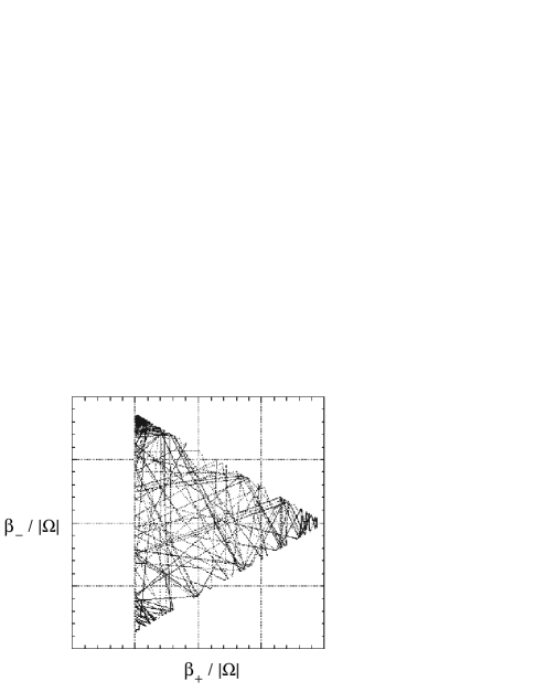
FIG. 1.: A typical Mixmaster trajectory as projected into the anisotropy plane. The rescaled variables (Moser et al (1971)) cause the bounces to occur at fixed locations. More than 262 bounces are shown (see Berger, Garfinkle, and Strasser (1997)).

The case $V\equiv 0$ corresponds in fact to the Kasner solution (Bianchi Type I with $C^{i}_{jk}=0$). Thus Eq. (4) may be replaced by $H_{K}$ whose variation yields in the limit $\Omega\to-\infty$,

$$\beta_{\pm}={{p_{\pm}}\over{|p_{\Omega}|}}|\Omega|.$$ (10)

However, we require from Eq. (7) (now $H_{K}=0$)

$$p_{\Omega}^{2}=p_{+}^{2}+p_{-}^{2}$$ (11)

and can replace Eq. (8) with

$$\beta_{+}=\cos\theta|\Omega|\quad,\quad\beta_{-}=\sin\theta|\Omega|.$$ (12)

If the Mixmaster model were AVTD, substitution of Eq. (10) into Eq. (5) would yield only terms which decay exponentially as $\Omega\to-\infty$.

Consider the first term on the right hand side (rhs) of Eq. (5). Upon substitution with Eq. (10), we find

$$e^{4\Omega-8\beta_{+}}\to e^{-4|\Omega|(1+2\cos\theta)}.$$ (13)

If $\cos\theta<-{\textstyle{1\over 2}}$, this term will grow exponentially. A bounce off this exponential wall then occurs leading to a new value for $\cos\theta$. Conservation of momentum yields (Ryan (1971))

$$\cos\theta^{\prime}=-{{4+5\cos\theta}\over{5+4\cos\theta}}$$ (14)

which causes the first term on the rhs of Eq. (5) to exponentially decay. However, depending on the sign of $\sin\theta$, either the second or third term on the rhs of Eq. (5) will begin to grow exponentially. This process repeats indefinitely. Numerical studies (Moser et al (1973), Rugh and Jones (1990), Berger, Garfinkle, and Strasser (1997)) confirm this picture (see Fig. 1). This means that all terms which were neglected in the MCP are in fact negligible.

III Gowdy universes on $T^{3}\times R$

If spatial dependence in one direction (e.g. on $0\leq\theta\leq 2\pi$) is allowed in the anisotropic scale factors of a Bianchi I homogeneous cosmology, the $T^{3}\times R$ Gowdy (1971) solution is obtained (see also Berger (1974)). The metric

$$ds^{2}=e^{-\lambda/2}e^{\tau/2}(-e^{-2\tau}d\tau^{2}+d\theta^{2})+e^{-\tau}[e^{P}d\sigma^{2}+2e^{P}Q\,d\sigma\kern 1.0ptd\delta+(e^{P}Q^{2}+e^{-P})d\delta^{2}]$$ (15)

describes amplitudes $P(\theta,\tau)$ and $Q(\theta,\tau)$ for the $+$ and $\times$ polarizations of gravitational waves propagating in an inhomogeneous background spacetime written in terms of $\lambda(\theta,\tau)$. This model has the extremely nice property that the dynamical equations for the waves obtained by variation of the (non-zero) Hamiltonian (Moncrief (1981))

$$H=\oint{d\theta\left({{\textstyle{1\over 2}}\pi_{P}^{2}+{\textstyle{1\over 2}}e^{-2P}\pi_{Q}^{2}}\right)}+\oint{d\theta\,\left({{\textstyle{1\over 2}}e^{-2\tau}P,_{\theta}^{2}+{\textstyle{1\over 2}}e^{2(P-\tau)}Q,_{\theta}^{2}}\right)}=H_{K}+H_{V}$$ (16)

decouple from the constraints. Here $\pi_{P}$ and $\pi_{Q}$ are the momenta conjugate to $P$ and $Q$ respectively. The constraints are first order equations for $\lambda$ which can be solved trivially in terms of the $P$ and $Q$ found as solutions to the wave equations obtained from Eq. (14).

To use the MCP, we obtain the AVTD solution as $\tau\to\infty$ by variation of $H_{K}$ from Eq. (14). This yields

$$P\to v(\theta)\tau\quad,\quad Q\to Q_{0}(\theta).$$ (17)

Consider substitution in the separate terms of Eq. (14). The potential

$$V_{1}=\pi_{Q}^{2}e^{-2P}$$ (18)

in $H_{K}$ becomes

$$V_{1}=\pi_{Q}^{2}e^{-2v\tau}$$ (19)

which decays exponentially only for $v>0$. On the other hand,

$$V_{2}=Q,_{\theta}^{2}e^{2(P-\tau)}$$ (20)

in $H_{V}$ becomes

$$V_{2}=Q,_{\theta}^{2}e^{2(v-1)\tau}$$ (21)

which decays exponentially if $v<1$. Thus we see that $0<v<1$ (at each spatial point) is consistent as $\tau\to\infty$ with an AVTD singularity.

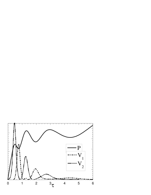
FIG. 2.: $P$, $V_{1}$, and $V_{2}$ vs $\tau$ at a fixed value of $\theta$. Note that the slope of $P$, $P,_{\tau}$, decreases after each interaction with $V_{2}$ while $P,_{\tau}$ goes from negative to positive after each interaction with $V_{1}$. A continuation of this graph in $\tau$ would show that $V_{1}$ and $V_{2}$ have permanently died off and that $P$ continues to increase with fixed positive slope $P,_{\tau}<1$.

What happens if $P,_{\tau}<0$ or $P,_{\tau}>1$? Then either $V_{1}$ or $V_{2}$ will be large. A bounce off each potential will drive $P,_{\tau}$ into the range allowed by that potential. Alternate bounces off both potentials will eventually drive $P,_{\tau}$ into the required range. This process is shown at a typical spatial point in Fig. 2 which is taken from a numerical simulation (Berger and Moncrief (1993), Berger and Garfinkle (1997)).

We note that exceptional behavior can occur at isolated spatial points where a coefficient of $V_{1}$ or $V_{2}$ (i.e. $\pi_{Q}$ or $Q,_{\theta}$) vanishes. Since near these exceptional points $V_{1}$ or $V_{2}$ is small, the mechanism to drive $P,_{\tau}$ into the range $(0,1)$ takes a very long time to become effective. This means that $P,_{\tau}>1$ or $P,_{\tau}<0$ can persist leading to the development of spiky features in $P$ and $Q$. These are discussed in detail elsewhere (Berger and Garfinkle (1997)).

The MCP combined with numerical simulations provide strong evidence that the Gowdy singularity is AVTD except, perhaps, at isolated spatial points.

IV $U(1)$ symmetric cosmologies on $T^{3}\times R$

We have also considered a class of cosmologies with dependence on two spatial variables $u$, $v$ as well as time $\tau$. The model may be described by five degrees of freedom $\{z,x,\varphi,\omega,\Lambda\}$ with conjugate momenta $\{p_{z},p_{x},p_{\varphi},p_{\omega},p_{\Lambda}\}$. The metric takes the form (Moncrief (1986), Berger and Moncrief (1993))

$$ds^{2}=e^{-2\varphi}\left\{{-N^{2}e^{-4\tau}d\tau^{2}+e^{-2\tau}e^{\Lambda}e_{ab}dx^{a}dx^{b}}\right\}+e^{2\varphi}\left({dx^{3}+\beta_{a}dx^{a}}\right)^{2}$$ (22)

where $\{x^{a}\}=\{u,v\}$, $N=e^{\Lambda}$, $x^{3}$ is the symmetry direction and

$$e_{ab}={\textstyle{1\over 2}}\left({\matrix{{e^{2z}+e^{-2z}(1+x)^{2}}&{e^{2z}+e^{-2z}(x^{2}-1)}\cr{e^{2z}+e^{-2z}(x^{2}-1)}&{e^{2z}+e^{-2z}(1-x)^{2}}\cr}}\right)$$ (23)

is the conformal metric in the $u$-$v$ plane. The variable $\omega$ is obtained from a canonical transformation of the twists $\beta^{a}$. Einstein’s equations are obtained from the variation of

$$H = \oint{\oint{dudv}}\left({{\textstyle{1\over 8}}p_{z}^{2}+{\textstyle{1\over 2}}e^{4z}p_{x}^{2}+{\textstyle{1\over 8}}p_{\varphi}^{2}+{\textstyle{1\over 2}}e^{4\varphi}p_{\omega}^{2}-{\textstyle{1\over 2}}p_{\Lambda}^{2}+2p_{\Lambda}}\right)+e^{-2\tau}\oint{\oint{dudv}}\left\{{\left({e^{\Lambda}e^{ab}}\right),_{ab}-\left({e^{\Lambda}e^{ab}}\right),_{a}\Lambda,_{b}}\right.$$ (25)

$$+e^{\Lambda}\left[{\left({e^{-2z}}\right),_{u}x,_{v}-\left({e^{-2z}}\right),_{v}x,_{u}}\right]+\left.{2e^{\Lambda}e^{ab}\varphi,_{a}\varphi,_{b}+{\textstyle{1\over 2}}e^{\Lambda}e^{-4\varphi}e^{ab}\omega,_{a}\omega,_{b}}\right\}=H_{K}+H_{V}.$$

Unfortunately, the constraints are nontrivial. So far, we only have a restricted solution to them initially and have not yet implemented a program to enforce them during numerical evolution. (Constraint preservation is guaranteed analytically but not in a differenced approximation to Einstein s equations.)

Despite the complicated appearance of Eq. (22), the MCP may still be used. Variation of $H_{K}$ in Eq. (22) yields as $\tau\to\infty$ the AVTD solution

$$z\to-v_{z}(u,v)\tau\quad,\quad x\to x_{0}(u,v)\quad,\quad\varphi\to-v_{\varphi}(u,v)\tau\quad,\quad\omega\to\omega_{0}(u,v)\quad,$$ (26)

$$\Lambda\to\Lambda_{0}(u,v)+[2-p_{\Lambda}^{0}(u,v)]\tau\quad,\quad p_{z}\to-4v_{z}(u,v)\quad,\quad p_{x}\to p_{x}^{0}(u,v)\quad,$$ (27)

$$p_{\varphi}\to-4v_{\varphi}(u,v)\quad,\quad p_{\omega}\to p_{\omega}^{0}(u,v)\quad,\quad p_{\Lambda}\to p_{\Lambda}^{0}(u,v)\quad.$$ (28)

In the AVTD limit, the Hamiltonian constraint becomes

$$\tilde{H}_{K}=2v_{z}^{2}+{\textstyle{1\over 2}}e^{-4v_{z}}(p_{x}^{0})^{2}+2v_{\varphi}^{2}+{\textstyle{1\over 2}}e^{-4v_{\varphi}}(p_{\omega}^{0})^{2}-{\textstyle{1\over 2}}(p_{\Lambda}^{0})^{2}=0.$$ (29)

The exponential terms in $\tilde{H}_{K}$ decay only for $v_{z}>0$ and $v_{\varphi}>0$ as in the Gowdy spacetime and will act to drive $z,_{\tau}$ and $\varphi,_{\tau}$ into the allowed range. We require $p_{\Lambda}^{0}>0$ to enforce collapse. Thus we need only consider the restriction

$$\tilde{H}_{K}=2v_{z}^{2}+2v_{\varphi}^{2}-{\textstyle{1\over 2}}(p_{\Lambda}^{0})^{2}=0$$ (30)

as $\tau\to\infty$. Although $H_{V}$ is complicated, there are only two types of exponential dependence. Schematically, for $H_{V}=\oint{\oint{dudv}}\,V$,

$$V\approx Ce^{\Lambda-2\tau-2z}+e^{\Lambda-2\tau-2z-4\varphi}(\nabla\omega)^{2}.$$ (31)

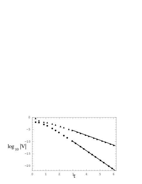
FIG. 3.: The logarithm of the non-schematic $V$ (from Eq. (22)) vs $\tau$ for a polarized $U(1)$ model. The solid lines are exponential best fits.

Only the term in Eq. (22) containing spatial derivatives of $\omega$ has the behavior shown in the second term on the rhs of Eq. (26). The others all behave as the first term. Substitution of the AVTD solution Eq. (23) and the restriction given by Eq. (25) yield (again schematically)

$$V\approx Ce^{-2v_{\varphi}\tau}+e^{2v_{\varphi}\tau}(\nabla\omega)^{2}.$$ (32)

The special case of polarized $U(1)$ models have $\omega=p_{\omega}=0$. This is the only degree of freedom that may be permanently removed (both analytically and numerically). In this case,

$$V\approx Ce^{-2v_{\varphi}\tau}.$$ (33)

Thus we expect polarized models to have AVTD singularities (Grubis̆ić and Moncrief (1994)). The numerical simulations verify this prediction (Berger, Garfinkle, and Moncrief (1997), Berger and Moncrief (1997)). Fig. 3 shows the exponential decay of $V$ at two typical spatial points. Behaviors of $\Lambda$, $z$, $x$, and $\varphi$ are also consistent with an AVTD singularity.

For generic models, Eq. (27) predicts a growing term in $V$. This means that if a collapsing spacetime tries to become AVTD, a potential term will grow exponentially. A bounce off this potential will (among other things) change the sign of $\varphi,_{\tau}$ so that an exponential term in $\tilde{H}_{K}$ will grow. The process should repeat indefinitely since neither $v_{\varphi}>0$ nor $v_{\varphi}<0$ is consistent with both terms exponentially small.

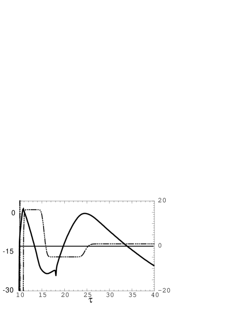
FIG. 4.: The potential $V$ vs $\tau$ The base-10 logarithm of the (non-schematic—i.e. from Eq. (22)) second term on the rhs of Eq. (27) is plotted (solid line, left scale). Note the exponentially growing and decaying portions of the graph. Also plotted (broken line) is the combination of momenta $(p_{\Lambda}+p_{\varphi}+p_{z}/2)$ that yields the negative of the quantity that multiplies $\tau$ in the AVTD limit. The horizontal line indicates zero for this quantity (right scale).

Results from a simulation (Fig. 4) appear to be consistent with this picture which itself is in accord with the BKL conjecture. However, there is a large caveat. The exponents in $V$ in Eq. (26) are regulated by the kinetic part of the Hamiltonian constraint Eq. (25). If the value of $\tilde{H}_{K}$ is incorrect due to numerical error, the exponent may have the wrong sign yielding qualitatively wrong behavior. Thus these models will not provide information on the validity of the BKL conjecture until enforcement of the constraint is implemented. In polarized $U(1)$ models, the result is much stronger because the constraints remain small (and converge to zero with increasing spatial resolution) for all $\tau$ (Berger and Moncrief (1997))).

A cleaner example of very similar behavior in one spatial dimension will be discussed elsewhere (Weaver et al (1997)).

V Conclusions

We explore the behavior of cosmological spacetimes in their collapse to a singularity. The MCP can predict whether the singularity will be AVTD or Mixmaster-like. In the Gowdy case, we learn how the nonlinearities in the wave equations force the parameters into the range for consistent AVTD behavior. At isolated spatial points, these terms are absent so non-generic behavior can occur. This leads to the growth of spiky features.

In polarized $U(1)$ cosmologies, these spiky features do not arise. Numerical evolutions support the prediction that these models are AVTD. In generic $U(1)$ models, we expect a Mixmaster-like singularity. Numerical difficulties prevent a definitive conclusion in this case although there is some evidence to support this claim.

We emphasize that, to the extent we believe the numerical results, the character of the singularity is completely local. The predictions of the MCP assume constancy in time of the spatially dependent coefficients of the exponentially growing or decaying terms. Simulations support such behavior sufficiently close to the singularity.

While the singularity occurs at (say) $\tau=\infty$, we have performed numerical simulations only to some $\tau_{F}<\infty$. Nonetheless, we believe that we can use these simulations to support conjectures about the nature of singularities in these models. Since the numerical simulations support predictions based on the MCP, we argue that we understand the effect of all the nonlinear terms on the evolution toward the singularity. It seems reasonable to suppose that for $\tau_{F}<\tau<\infty$ nothing qualitatively different will happen. This is almost certainly true for AVTD spacetimes. An infinite sequence of Mixmaster bounces at different spatial points could yield eventually a very complicated spatial structure (e.g. Kirillov and Kochnev (1987)). It is likely, nevertheless, that the exponential potentials will still dominate over increasing spatial derivatives as the controlling factor in the evolution.

REFERENCES

- [1] Belinskii, V. A., Lifshitz, E. M. and Khalatnikov, I. M. (1971), Oscillatory Approach to the Singular Point in Relativistic Cosmology, Sov. Phys. Usp., 13: 74–765.
- [2] Berger, B. K. (1974), Quantum Graviton Creation in a Model Universe, Ann. Phys. (N.Y.), 83: 458.
- [3] Berger, B. K. and Garfinkle, D. (1997), Phenomenology of the Gowdy Model on , gr-qc/9710102.
- [4] Berger, B. K., Garfinkle, D., and Moncrief, V. (1997), Numerical Study of Cosmological Singularities, gr-qc/9709073.
- [5] Berger, B. K., Garfinkle, D., and Strasser, E. (1997), New Algorithm for Mixmaster Dynamics, Class. Quantum Grav., 14, L29–L36.
- [6] Berger, B. K. and Moncrief, V. (1993), Numerical Investigation of Cosmological Singularities, Phys. Rev. D, 48: 4676.
- [7] Berger, B. K. and Moncrief, V. (1997), Numerical Evidence for Velocity Dominated Singularities in Polarized Symmetric Cosmologies, unpublished.
- [8] Gowdy, R. H. (1971), Gravitational Waves in Closed Universes, Phys. Rev. Lett., 27: 826.
- [9] Grubis̆ić, B. and Moncrief, V. (1993), Asymptotic Behavior of the Gowdy Space-times, Phys. Rev. D, 47, 2371–2382.
- [10] Grubis̆ić, B. and Moncrief, V. (1994), Mixmaster Spacetime, Geroch’s Transformation, and Constants of Motion, Phys. Rev. D, 49, 2792–2800.
- [11] Hawking, S. W. and Penrose, R. (1970), The Singularities of Gravitational Collapse and Cosmology, Proc. Roy. Soc. Lond. A, 314: 529–548.
- [12] Isenberg, J. A. and Moncrief, V. (1990), Asymptotic Behavior of the Gravitational Field and the Nature of Singularities in Gowdy Spacetimes, Ann. Phys. (N.Y.), 199: 84.
- [13] Kirillov, A. A. and Kochnev, A. A. (1987), Cellular Structure of Space near a Singularity in Time in Einstein’s Equations, JETP Lett., 46, 435–438.
- [14] Misner, C. W. (1969), Mixmaster Universe, Phys. Rev. Lett., 22: 1071–1074.
- [15] Moncrief, V. (1981), Global Properties of Gowdy Spacetimes with Topology, Ann. Phys. (N.Y.), 132, 87–10.
- [16] Moncrief, V. (1986), Reduction of Einstein’s Equations for Vacuum Space-Times with Spacelike Isometry Groups, Ann. Phys. (N.Y.), 167: 118.
- [17] Moser, A.R., Matzner, R.A. and Ryan, M.P., Jr. (1973), Numerical Solutions for Symmetric Bianchi Type IX Universes, Ann. Phys. (N.Y.), 79, 558–579.
- [18] Rugh, S.E. and Jones, B.J.T. (1990), Chaotic Behaviour and Oscillating Three-Volumes in Bianchi IX Universes, Phys. Lett., A147, 353–359.
- [19] Ryan, M. P., Jr. (1971), Qualitative Cosmology: Diagrammatic Solutions for Bianchi Type IX Universes with Expansion, Rotation, and Shear. I. The Symmetric Case, Ann. Phys. (N.Y.), 65, 506–537.
- [20] Weaver, M., Isenberg, J., and Berger, B.K. (1997), Mixmaster Behavior in Inhomogeneous Cosmological Spacetimes, gr-qc/9712055.