Solution to the inverse problem for a noisy spherical gravitational wave antenna

Abstract

A spherical gravitational wave antenna is distinct from other types of gravitational wave antennas in that only a single detector is necessary to determine the direction and polarization of a gravitational wave. Zhou and Michelson showed that the inverse problem can be solved using the maximum likelihood method if the detector outputs are independent and have normally distributed noise with the same variance. This paper presents an analytic solution using only linear algebra that is found to produce identical results as the maximum likelihood method but with less computational burden. Applications of this solution to gravitational waves in alternative symmetric metric theories of gravity and impulsive excitations also are discussed.

I Introduction

Several resonant-mass gravitational wave antennas are now in continuous operation with strain sensitivities of the order $10^{-21}\text{Hz}^{-1/2}$ [1]. With further improvements to these detectors and the addition of several large laser interferometers now under construction [2], the prospects for gravitational wave astronomy are quite good. The underlying non-gravitational physics associated with these detectors is reasonably understood and further improvements can be based on solid technological guidelines.

Many believe the next generation of resonant-mass antennas will be of spherical shape [3]. Confirmed detection of gravitational waves will require a coincidence between several detectors, thus the unique features of a sphere may play an essential role in a network of gravitational wave antennas. Two important features of a sphere are its equal sensitivity to gravitational waves from all directions and polarizations and its ability to determine the directional information and tensorial character of a gravitational wave [4].

To take full advantage of these capabilities, one needs to be able to interpret the data such a detector will produce. Recently, much work has been done to understand the output of a spherical antenna equipped with resonant transducers [5, 6]. All of these proposals operate on the principle that the response of the transducers can be transformed into a quantity that has a one-to-one correspondence with the tensorial components of a gravitational wave. With the measurement of these components, it is possible to solve the inverse problem to obtain the direction and polarization amplitudes of a gravitational wave.

The solution to the inverse problem for a noiseless spherical antenna first was outlined in the mid 1970’s by Wagoner and Paik [4]. More recently, the solution for a network of five noiseless bar antennas or interferometers was solved by Dhurandhar and Tinto [7]. This method assumed that the detectors were co-located but oriented in different directions. This solution is quite elegant because the exact solution can be found using straightforward algebra. Since a sphere can be thought of as five bar detectors occupying the same space, this solution can be adapted for a spherical antenna [8, 9]. In addition, Lobo outlined a procedure that can be used if the correct theory of gravity is not general relativity but unknown [10]. What all these proposals have in common is that they use basic symmetry properties of the matrices describing the detectors and their response to a gravitational wave. This makes them intuitive and easy to visualize [11].

The solution to the inverse problem in the presence of noise is more complicated. Gürsel and Tinto solved the problem for three noisy interferometers using a maximum likelihood method [12]. This solution required the measurement of the time delay of the signal between widely separated detectors to triangulate the direction of the source. Zhou and Michelson showed that the inverse problem for a spherical antenna can be solved in the presence of noise, also using a maximum likelihood method [8].

What is disappointing about the maximum likelihood method is that the original simplicity of Dhurandhar and Tinto’s noiseless solution is lost. In addition, an exact solution for the spherical detector was not found, making it necessary to solve the problem numerically. This solution can be computationally expensive, especially if the signal-to-noise ratio (SNR) is low. For the three interferometer case, the numerical solution often can lead to an incorrect estimate at low SNR [12]. This appears not to be a problem for a spherical antenna; a global maximum usually exists and is aligned with the correct direction. This leads us to believe that the problem for a spherical antenna can be solved analytically.

On experiments with the room-temperature prototype spherical antenna (TIGA) at Louisiana State University, we used a procedure to solve the inverse problem for impulsive excitations applied to the sphere surface [13, 14]. This solution was similar to Dhurandhar and Tinto’s original solution for gravitational waves, but we used a perturbation argument (presented below) to take into account the finite SNR of the experiment. The case of an impulsive excitation is more simple than a gravity wave because fewer parameters are involved, however, we show below that this method also can be used to find an analytic solution for gravitational waves.

We begin by reviewing the response of a spherical antenna to gravitational waves in general relativity and show how Dhurandhar and Tinto’s original method can be applied to solve for the wave direction and polarization amplitudes. We then generalize the arguments to any symmetric metric theory of gravity as well as to impulsive excitations. In Sec. III we show how this technique can be extended to a noisy antenna with independent and equally sensitive detector outputs. This solution is found to be equivalent to the maximum likelihood method under the same noise requirements. The general approach taken allow this solution to be easily adapted to other types of excitations with similar symmetry properties. We conclude the paper with a discussion of the limitations of the solution and possible extensions of this method.

II Detector response of an elastic sphere

Dhurandhar and Tinto solved the inverse problem for 5 bar antennas as well as 5 interferometers [7]. Others have used their method to solve the problem for a spherical antenna [8, 9]. Their technique involves constructing a matrix, say $\textstyle A$, that describes the response of the detector to a gravitational wave. They found that in general relativity the eigenvector of $\textstyle A$ with zero eigenvalue points in the propagation direction of the wave. In the following we will also use this concept, but will derive the equations in the context of linear algebra as this will lead us directly into the solution for the noisy antenna. For a more complete discussion of the response of an elastic sphere to gravitational waves the reader is referred to Refs. [15, 16, 10].

A Detector response in general relativity

A gravitational wave is a traveling time-dependent deviation of the metric perturbation, denoted by $H_{\mu\nu}(t)$. We follow a common textbook development for the metric deviation of a gravitational wave, which finds that only the spatial components $H_{ij}(t)$ are non-zero, and further can be taken to be transverse and traceless [17]. This tensor is simplified if we initially write it in the “wave-frame,” denoted by primed coordinates and indices. This is a coordinate frame with origin at the center of mass of the detector and the $z^{\prime}$ axis aligned to the propagation direction of the wave. We restrict ourselves to detectors much smaller than the gravitational wavelength so only the time dependence of $H_{ij}(t)$ will have significant physical effects. A general form for the spatial components of the metric deviation in the wave-frame can be written as

$$\mathchoice{{\hbox{\boldmath$\displaystyle H$}}}{{\hbox{\boldmath$\textstyle H$}}}{{\hbox{\boldmath$\scriptstyle H$}}}{{\hbox{\boldmath$\scriptscriptstyle H$}}}^{\prime}(t)=\left[\begin{array}[]{ccc}h_{+}(t)&h_{\times}(t)&0\\ h_{\times}(t)&-h_{+}(t)&0\\ 0&0&0\end{array}\right],$$ (1)

where $h_{+}(t)$ and $h_{\times}(t)$ are the wave amplitudes for the two allowed states of linear polarization and are called the plus and cross amplitudes.

The detector is more easily described in the “lab-frame,” denoted by unprimed coordinates and indices, with origin at the center of mass of the detector and the $z$ axis aligned with the local vertical. In this frame, the primary physical effect of a passing gravitational wave is to produce a time dependent “tidal” force density $f^{\text{GW}}(\mathchoice{{\hbox{\boldmath$\displaystyle x$}}}{{\hbox{\boldmath$\textstyle x$}}}{{\hbox{\boldmath$\scriptstyle x$}}}{{\hbox{\boldmath$\scriptscriptstyle x$}}},t)$ on the material with mass density $\rho$ at coordinate location $x_{i}$. This force is related to the metric perturbation by

$$f^{\text{GW}}_{i}(\mathchoice{{\hbox{\boldmath$\displaystyle x$}}}{{\hbox{\boldmath$\textstyle x$}}}{{\hbox{\boldmath$\scriptstyle x$}}}{{\hbox{\boldmath$\scriptscriptstyle x$}}},t)=\frac{1}{2}\rho\sum_{j}\ddot{H}_{ij}(t)x_{j}.$$ (2)

It is natural to look for an alternate expression that separates the coordinate dependence into radial and angular parts. Because the tensor $H_{ij}(t)$ is traceless, the angular expansion can be done completely with the five second order real valued spherical harmonics $Y_{2m}(\theta,\phi)$, where the index $m=1\ldots 5$. We call the resulting time dependent expansion coefficients, denoted by $h_{m}(t)$, the “spherical amplitudes” [16]. They are a complete and orthogonal representation of the cartesian metric deviation tensor $H_{ij}(t)$. They depend only on the two wave-frame amplitudes and the direction of propagation.

To transform the metric perturbation to the lab-frame we perform the appropriate rotations using the y-convention of the Euler angles shown in Fig. 1. We denote the rotation about the wave $z^{\prime}$ axis by $\alpha$, the rotation about the new $y$ axis ($\eta^{\prime}$) by $\beta$, and the rotation about the final lab $z$ axis by $\gamma$. The rotation matrix for the y-convention is

$$\mathchoice{{\hbox{\boldmath$\displaystyle R$}}}{{\hbox{\boldmath$\textstyle R$}}}{{\hbox{\boldmath$\scriptstyle R$}}}{{\hbox{\boldmath$\scriptscriptstyle R$}}}=\left[\begin{array}[]{ccc}\cos{\gamma}\cos{\beta}\cos{\alpha}-\sin{\gamma}\sin{\alpha}&\cos{\gamma}\cos{\beta}\sin{\alpha}+\sin{\gamma}\cos{\alpha}&-\cos{\gamma}\sin{\beta}\\ -\sin{\gamma}\cos{\beta}\cos{\alpha}-\cos{\gamma}\sin{\alpha}&-\sin{\gamma}\cos{\beta}\sin{\alpha}+\cos{\gamma}\cos{\alpha}&\sin{\gamma}\sin{\beta}\\ \sin{\beta}\cos{\alpha}&\sin{\beta}\sin{\alpha}&\cos{\beta}\end{array}\right].$$ (3)

At this point we arbitrarily set the rotation $\alpha$ about the wave $z^{\prime}$ axis equal to zero; inclusion of this rotation will only “mix” the two polarizations of the wave. The spherical amplitudes can now be written in terms of the polarization amplitudes and the source direction

$$h_{1}(t) = h_{+}(t)\frac{1}{2}\left({1+\cos^{2}\beta}\right)\cos 2\gamma+h_{\times}(t)\cos\beta\sin 2\gamma,$$ (5)

$$h_{2}(t) = -h_{+}(t)\frac{1}{2}\left({1+\cos^{2}\beta}\right)\sin 2\gamma+h_{\times}(t)\cos\beta\cos 2\gamma,$$ (6)

$$h_{3}(t) = -h_{+}(t)\frac{1}{2}\sin 2\beta\sin\gamma+h_{\times}(t)\sin\beta\cos\gamma,$$ (7)

$$h_{4}(t) = h_{+}(t)\frac{1}{2}\sin 2\beta\cos\gamma+h_{\times}(t)\sin\beta\sin\gamma,$$ (8)

$$h_{5}(t) = h_{+}(t)\frac{1}{2}\sqrt{3}\sin^{2}\beta.$$ (9)

The mechanics of a spherical antenna can be described by ordinary elastic theory. One finds that the eigenfunctions of an uncoupled sphere can be written in terms of the spherical harmonics

$$\mathchoice{{\hbox{\boldmath$\displaystyle\Psi$}}}{{\hbox{\boldmath$\textstyle\Psi$}}}{{\hbox{\boldmath$\scriptstyle\Psi$}}}{{\hbox{\boldmath$\scriptscriptstyle\Psi$}}}_{n\ell m}(r,\theta,\phi)=\left({\alpha_{n\ell}(r)\mathchoice{{\hbox{\boldmath$\displaystyle\hat{r}$}}}{{\hbox{\boldmath$\textstyle\hat{r}$}}}{{\hbox{\boldmath$\scriptstyle\hat{r}$}}}{{\hbox{\boldmath$\scriptscriptstyle\hat{r}$}}}+\beta_{n\ell}(r)a\mathchoice{{\hbox{\boldmath$\displaystyle\nabla$}}}{{\hbox{\boldmath$\textstyle\nabla$}}}{{\hbox{\boldmath$\scriptstyle\nabla$}}}{{\hbox{\boldmath$\scriptscriptstyle\nabla$}}}}\right)Y_{\ell m}(\theta,\phi).$$ (10)

The radial eigenfunctions $\alpha_{n\ell}(r)$ and $\beta_{n\ell}(r)$ determine the motion in the radial and tangential directions respectively and depend on the radius $a$ and the material of the sphere [4, 16].

In general relativity, only the 5 quadrupole modes of vibration will strongly couple to the force density of a gravitational wave. For an ideal sphere they are all degenerate, having the same eigenfrequency, and are distinguished only by their angular dependence. The effective force $F_{12m}(t)$ that a gravitational wave will exert on a fundamental quadrupole mode $m$ of the sphere is given by the overlap integral between the eigenfunctions of the sphere and the gravitational tidal force

$$F_{12m}(t)\equiv\int{\mathchoice{{\hbox{\boldmath$\displaystyle\Psi$}}}{{\hbox{\boldmath$\textstyle\Psi$}}}{{\hbox{\boldmath$\scriptstyle\Psi$}}}{{\hbox{\boldmath$\scriptscriptstyle\Psi$}}}_{12m}(\mathchoice{{\hbox{\boldmath$\displaystyle x$}}}{{\hbox{\boldmath$\textstyle x$}}}{{\hbox{\boldmath$\scriptstyle x$}}}{{\hbox{\boldmath$\scriptscriptstyle x$}}})\cdot\mathchoice{{\hbox{\boldmath$\displaystyle f$}}}{{\hbox{\boldmath$\textstyle f$}}}{{\hbox{\boldmath$\scriptstyle f$}}}{{\hbox{\boldmath$\scriptscriptstyle f$}}}^{\text{GW}}(\mathchoice{{\hbox{\boldmath$\displaystyle x$}}}{{\hbox{\boldmath$\textstyle x$}}}{{\hbox{\boldmath$\scriptstyle x$}}}{{\hbox{\boldmath$\scriptscriptstyle x$}}},t)\,d^{3}x}=\frac{1}{2}\ddot{h}_{m}(t)\,M\,\chi a.$$ (11)

Each spherical component of the gravitational field determines uniquely the effective force on the corresponding mode of the sphere and they are all identical in magnitude. We can interpret the effective force $F_{12m}(t)$ in each mode as the product of: the physical mass of the sphere $M$, an effective length $\chi a$ (a fraction of the sphere radius), and the gravitational acceleration $\frac{1}{2}\ddot{h}_{m}(t)$. The value of the coefficient $\chi$ depends on the sphere material, but is typically $\simeq 0.6$ [16].

By monitoring the quadrupole modes of the sphere, one has a direct measurement of the effective force on the sphere and thus the spherical amplitudes of the gravitational wave. The standard technique for doing so on resonant detectors is to position resonant transducers on the surface of the sphere that strongly couple to the quadrupole modes. A number of proposals have been made for the type and positions of the transducers [5, 6, 8]. What all of these proposals have in common is that the outputs of the transducers are combined into “mode channels” $g_{m}(t)$ that are constructed to have a one-to-one correspondence with the quadrupole modes of the sphere and thus the spherical amplitudes of the gravitational wave [16, 18],

$$g_{m}(t)\propto F_{12m}(t)\propto h_{m}(t).$$ (12)

The mode channels can be collected to form a “detector response” matrix $\mathchoice{{\hbox{\boldmath$\displaystyle A$}}}{{\hbox{\boldmath$\textstyle A$}}}{{\hbox{\boldmath$\scriptstyle A$}}}{{\hbox{\boldmath$\scriptscriptstyle A$}}}(t)$ that in the absence of noise is equal to the cartesian strain tensor $\mathchoice{{\hbox{\boldmath$\displaystyle H$}}}{{\hbox{\boldmath$\textstyle H$}}}{{\hbox{\boldmath$\scriptstyle H$}}}{{\hbox{\boldmath$\scriptscriptstyle H$}}}(t)$ in the lab frame

$$\mathchoice{{\hbox{\boldmath$\displaystyle A$}}}{{\hbox{\boldmath$\textstyle A$}}}{{\hbox{\boldmath$\scriptstyle A$}}}{{\hbox{\boldmath$\scriptscriptstyle A$}}}(t)\equiv\left[\begin{array}[]{ccc}g_{1}(t)-\frac{1}{\sqrt{3}}g_{5}(t)&g_{2}(t)&g_{4}(t)\\ g_{2}(t)&-g_{1}(t)-\frac{1}{\sqrt{3}}g_{5}(t)&g_{3}(t)\\ g_{4}(t)&g_{3}(t)&\frac{2}{\sqrt{3}}g_{5}(t)\end{array}\right].$$ (13)

For the remainder of this discussion we drop the notation of time dependence $(t)$ for brevity.

The strain tensor in the lab frame $\textstyle H$ is a symmetric traceless matrix. Consequently, it can be orthogonally diagonalized and has an orthonormal set of three eigenvectors. One can construct from the eigenvectors a transformation matrix $\textstyle R$ that diagonalizes $\textstyle H$. The matrix $\textstyle R$ is also orthogonal, thus it can be considered a rotation matrix (it may also include a reflection). The physical interpretation of this transformation is to rotate the lab frame such that the $z$ axis points in the direction of the source. The matrix $\textstyle R$ (the eigenvectors) will tell us the angles of rotation and thus the direction of the wave.

In the wave frame, $\mathchoice{{\hbox{\boldmath$\displaystyle H$}}}{{\hbox{\boldmath$\textstyle H$}}}{{\hbox{\boldmath$\scriptstyle H$}}}{{\hbox{\boldmath$\scriptscriptstyle H$}}}^{\prime}$ is not normally diagonal but it can be diagonalized by rotating Eq. (1) about the propagation axes using the Euler angle $\alpha$. $\alpha$ may be a constant or a function of time depending upon the situation. This rotation changes the polarization components of the tensor but not the wave direction relative to the lab frame.

To calculate the rotation matrix $\textstyle R$ we need to solve the general eigenvalue equation for the strain tensor

$$\mathchoice{{\hbox{\boldmath$\displaystyle H$}}}{{\hbox{\boldmath$\textstyle H$}}}{{\hbox{\boldmath$\scriptstyle H$}}}{{\hbox{\boldmath$\scriptscriptstyle H$}}}\;\mathchoice{{\hbox{\boldmath$\displaystyle x$}}}{{\hbox{\boldmath$\textstyle x$}}}{{\hbox{\boldmath$\scriptstyle x$}}}{{\hbox{\boldmath$\scriptscriptstyle x$}}}=\lambda_{x}\mathchoice{{\hbox{\boldmath$\displaystyle x$}}}{{\hbox{\boldmath$\textstyle x$}}}{{\hbox{\boldmath$\scriptstyle x$}}}{{\hbox{\boldmath$\scriptscriptstyle x$}}}.$$ (14)

Since $\textstyle A$ and $\textstyle H$ are equal in the absence of noise we are free to substitute $\textstyle A$ in Eq. (14) for $\textstyle H$. By inspection of Eq. (1) we see that in general relativity the eigenvector of $\textstyle H$ with $\lambda_{x}=0$ points in the propagation direction of the wave. The direction can be calculated from this eigenvector by recognizing that it corresponds to the last column vector of $\textstyle R$ in Eq. (3). Dividing the elements of this column we find

$$\tan{\gamma}=-\frac{y}{x},$$ (15)

$$\tan{\beta}=\frac{y}{z}\frac{1}{\sin{\gamma}}.$$ (16)

The unusual minus sign in Eq. (15) comes from the use of the y-convention of the Euler angles. Expanding Eq. (14) for $\lambda_{x}=0$ and substituting in a particular choice of matrix elements from Eq. (13) we find

$$\tan{\gamma}=\frac{3g_{4}g_{3}-2\sqrt{3}g_{2}g_{5}}{2\sqrt{3}g_{1}g_{5}+2g_{5}^{2}+3g_{3}^{2}},$$ (17)

$$\tan{\beta}=\pm\frac{\sqrt{3}g_{3}g_{4}-2g_{5}g_{2}}{\sqrt{3}g_{1}g_{4}+g_{5}g_{4}+\sqrt{3}g_{3}g_{2}}\frac{1}{\sin{\gamma}}.$$ (18)

This solution is valid only for a noiseless antenna; it will fail otherwise because we can no longer replace $\textstyle H$ with $\textstyle A$ and their eigenvectors and eigenvalues will no longer be equal. The $\pm$ in Eq. (18) illustrates the unavoidable fact that a single sphere cannot distinguish between antipodal sources. This ambiguity is a characteristic of all gravity wave detectors, but can be removed by measuring the time delay of the signal between two widely separated antennas.

Once the direction is calculated we can determine the two polarization amplitudes by taking a linear combination of Eqs. (3). These equations are actually overdetermined so several solutions exist (we have 5 equations but only 4 unknowns). In the absence of noise any particular solution to them is valid, but in anticipation of the noisy case we will take a systematic approach to the solution.

We need only the angles $\beta$ and $\gamma$ to rotate $\textstyle H$ to $\mathchoice{{\hbox{\boldmath$\displaystyle H$}}}{{\hbox{\boldmath$\textstyle H$}}}{{\hbox{\boldmath$\scriptstyle H$}}}{{\hbox{\boldmath$\scriptscriptstyle H$}}}^{\prime}$, so at this point we again set $\alpha=0$. The amplitudes are found by equating them to the corresponding matrix elements of $\mathchoice{{\hbox{\boldmath$\displaystyle H$}}}{{\hbox{\boldmath$\textstyle H$}}}{{\hbox{\boldmath$\scriptstyle H$}}}{{\hbox{\boldmath$\scriptscriptstyle H$}}}^{\prime}$ in Eq. (1). Again, we may substitute $\textstyle A$ for $\textstyle H$ and $\mathchoice{{\hbox{\boldmath$\displaystyle A$}}}{{\hbox{\boldmath$\textstyle A$}}}{{\hbox{\boldmath$\scriptstyle A$}}}{{\hbox{\boldmath$\scriptscriptstyle A$}}}^{\prime}$ for $\mathchoice{{\hbox{\boldmath$\displaystyle H$}}}{{\hbox{\boldmath$\textstyle H$}}}{{\hbox{\boldmath$\scriptstyle H$}}}{{\hbox{\boldmath$\scriptscriptstyle H$}}}^{\prime}$ so we have $h_{+}=A_{11}^{\prime}=-A_{22}^{\prime}$ and $h_{\times}=A_{12}^{\prime}=A_{21}^{\prime}$. $\textstyle A$ and $\mathchoice{{\hbox{\boldmath$\displaystyle A$}}}{{\hbox{\boldmath$\textstyle A$}}}{{\hbox{\boldmath$\scriptstyle A$}}}{{\hbox{\boldmath$\scriptscriptstyle A$}}}^{\prime}$ are symmetric so $A_{12}^{\prime}$ and $A_{21}^{\prime}$ will always be identical even when noise is introduced. However, no such restriction is placed on $A_{11}^{\prime}$ and $A_{22}^{\prime}$. We will use the average $(A_{11}^{\prime}-A_{22}^{\prime})/2$ to calculate $h_{+}$ for reasons that will become clear later.

Multiplying $\mathchoice{{\hbox{\boldmath$\displaystyle A$}}}{{\hbox{\boldmath$\textstyle A$}}}{{\hbox{\boldmath$\scriptstyle A$}}}{{\hbox{\boldmath$\scriptscriptstyle A$}}}^{\prime}=\mathchoice{{\hbox{\boldmath$\displaystyle R$}}}{{\hbox{\boldmath$\textstyle R$}}}{{\hbox{\boldmath$\scriptstyle R$}}}{{\hbox{\boldmath$\scriptscriptstyle R$}}}^{T}\mathchoice{{\hbox{\boldmath$\displaystyle A$}}}{{\hbox{\boldmath$\textstyle A$}}}{{\hbox{\boldmath$\scriptstyle A$}}}{{\hbox{\boldmath$\scriptscriptstyle A$}}}\mathchoice{{\hbox{\boldmath$\displaystyle R$}}}{{\hbox{\boldmath$\textstyle R$}}}{{\hbox{\boldmath$\scriptstyle R$}}}{{\hbox{\boldmath$\scriptscriptstyle R$}}}$ for $\alpha=0$ and selecting the proper elements we find

$$h_{+}=g_{1}\frac{1}{2}(1+\cos^{2}{\beta})\cos{2\gamma}-g_{2}\frac{1}{2}(1+\cos^{2}{\beta})\sin{2\gamma}-g_{3}\frac{1}{2}\sin{2\beta}\sin{\gamma}+g_{4}\frac{1}{2}\sin{2\beta}\cos{\gamma}+g_{5}\frac{\sqrt{3}}{2}\sin^{2}{\beta}.$$ (19)

$$h_{\times}=g_{1}\cos{\beta}\sin{2\gamma}+g_{2}\cos{\beta}\cos{2\gamma}+g_{3}\sin{\beta}\cos{\gamma}+g_{4}\sin{\beta}\sin{\gamma}.$$ (20)

These equations can also be derived by taking a linear combination of Eqs. (3). This is not the only valid solution in the noiseless case, but it is particularly symmetric: the coefficients of each component $g_{m}$ is the same as the corresponding coefficients of $h_{+}$ or $h_{\times}$ in Eqs. (3) for $h_{m}$. The fact that $h_{\times}$ does not contain a $g_{5}$ contribution is an artifact of using the y-convention of the Euler angles; in other conventions this term may be non-zero.

B Detector response in alternative theories of gravity

Experiments in the solar system and pulsar-timing tests have ruled out many competing theories of gravity, however, general relativity is not the only theory of gravity that passes these weak field tests [19]. One measurement that can potentially rule out certain gravitational theories is the properties of gravitational waves [20], such as the speed of propagation and allowable polarization states. It was shown above how a single sphere can measure the quadrupole components of the strain tensor, but a scalar wave can excite both the monopole mode and the quadrupole modes of a sphere [10, 21]. By monitoring both types of modes, a single spherical detector can measure all the tensor components of a gravitational wave. This makes it possible for a single spherical detector to determine all of the six polarization states predicted by the most general symmetric metric theory of gravity [22].

We can rewrite Eq. (11) in terms of the electric components of the Riemann tensor [20] $E_{ij}=R_{0i0j}$,

$$F_{n\ell m}=-\frac{1}{M}E_{ij}\int\Psi_{n\ell m}^{i}x^{j}\rho d^{3}x,$$ (21)

where we now include both the $\ell=2$ quadrupole modes and the $\ell=0$ monopole mode. The monopole mode of an elastic sphere is actually at a higher frequency than the quadrupole modes. If the source is not wide-band enough for detection in both of these modes, a second sphere with the monopole mode tuned to the quadrupole modes of the first will be needed to measure this component. If the first sphere is at relatively low frequency, one might consider making the second sphere hollow to keep it of a practical size [23]. An alternative to a second sphere is to monitor the $n=2$ quadrupole modes and the monopole mode of a single sphere. These modes are not far in frequency from each other and also have relatively large cross-sections [24, 10].

Expanding Eq. (21) into radial and angular parts we find an additional spherical amplitude $h_{0}$ corresponding to the $\ell=0$ spherical harmonic. The detector response in the lab frame can now be written as

$$\mathchoice{{\hbox{\boldmath$\displaystyle A$}}}{{\hbox{\boldmath$\textstyle A$}}}{{\hbox{\boldmath$\scriptstyle A$}}}{{\hbox{\boldmath$\scriptscriptstyle A$}}}\equiv\left[\begin{array}[]{ccc}g_{1}-\frac{1}{\sqrt{3}}g_{5}+g_{0}&g_{2}&g_{4}\\ g_{2}&-g_{1}-\frac{1}{\sqrt{3}}g_{5}+g_{0}&g_{3}\\ g_{4}&g_{3}&\frac{2}{\sqrt{3}}g_{5}+g_{0}\end{array}\right].$$ (22)

To determine how to solve the inverse problem we need to examine the form of $E_{ij}$. It is a symmetric tensor so it has only six independent components. It can be written in terms of the complex Newman-Penrose parameters [25] which allow the identification of the spin content of the metric theory responsible for the generation of the wave

$$E_{ij}=\left[\begin{array}[]{ccc}-\Re\Psi_{4}-\Phi_{22}&\Im\Psi_{4}&-\sqrt{8}\Re\Psi_{3}\\ \Im\Psi_{4}&\Re\Psi_{4}-\Phi_{22}&\sqrt{8}\Im\Psi_{3}\\ -\sqrt{8}\Re\Psi_{3}&\sqrt{8}\Im\Psi_{3}&-6\Psi_{2}\end{array}\right].$$ (23)

We can divide the theories of gravity into categories using the E(2) classification scheme shown in Tab. I [26]. The tensor $E_{ij}$ is symmetric for all of these classes, thus it is orthogonally diagonalizable, but classes $II_{6}$ and $III_{5}$ have more degrees of freedom (direction plus polarization states) than we are capable of measuring with a single spherical detector. These two classes are often referred to as “observer-dependent” because different observers will disagree upon which polarization states are present. As a consequence, the polarization amplitudes for a particular observer must be known before the direction of the wave can be estimated.

For the “observer-independent” classes $O_{0}$, $O_{1}$, $N_{2}$, and $N_{3}$, the situation is more straightforward. $O_{0}$ is obviously uninteresting as it does not predict any gravitational waves (this class along with $O_{1}$ have essentially been ruled out by previous experiments [19]). We notice that $E_{ij}$ for the observer-independent classes can be diagonalized by a rotation $\alpha$ about the propagation axis, therefore, we can use the same arguments presented above for general relativity to solve for the wave direction.

The most general observer-independent class is $N_{3}$, which has

$$E_{ij}=\left[\begin{array}[]{ccc}-\Re\Psi_{4}-\Phi_{22}&\Im\Psi_{4}&0\\ \Im\Psi_{4}&\Re\Psi_{4}-\Phi_{22}&0\\ 0&0&0\end{array}\right].$$ (24)

Looking at the form of $E_{ij}$ we see that the same procedure for calculating the direction of the wave in general relativity holds for all the observer-independent classes: the eigenvector of $\textstyle A$ with eigenvalue equal to zero points at the source. The one exception to this statement is the case where the driving forces remain in a fixed line, for example $\Im\Psi_{4}=0,\Re\Psi_{4}=\Phi_{22}$. In this situation the direction of the wave can only be determined within the plane defined by the two eigenvectors with eigenvalues equal to zero.

C Detector response to impulsive excitations

Impulsive excitations are often used on resonant-mass detectors to calibrate the antenna [27]. The excitations are usually administered by either a short electrical burst applied to a calibrator attached to the surface or a hammer blow. Impulsive excitations were also used to test the analysis techniques used for experiments with the prototype spherical antenna at Louisiana State University [13, 14].

A radial impulse excitation can be easily described if we choose the $z^{\prime}$ axis to be along the direction of the impulse. By examining the quadrupole eigenfunctions of the sphere in this frame we notice that out of these modes only the $\Psi_{125}$ mode will be excited (other sphere modes will also be excited but their response can be removed by narrow-band filtering). All of the other quadrupole modes have a vanishing radial component of their eigenfunctions at this location which makes their “overlap” integral with the impulse vanish. In this frame the detector response is

$$\mathchoice{{\hbox{\boldmath$\displaystyle A$}}}{{\hbox{\boldmath$\textstyle A$}}}{{\hbox{\boldmath$\scriptstyle A$}}}{{\hbox{\boldmath$\scriptscriptstyle A$}}}^{\prime}=\left[\begin{array}[]{ccc}-\frac{1}{\sqrt{3}}g_{5}^{\prime}&0&0\\ 0&-\frac{1}{\sqrt{3}}g_{5}^{\prime}&0\\ 0&0&\frac{2}{\sqrt{3}}g_{5}^{\prime}\end{array}\right].$$ (25)

In the lab frame $\textstyle A$ is still given by Eq. (13).

Again, the direction can be found by calculating the eigenvalues and eigenvectors of the lab frame $\textstyle A$. In the absence of noise, the eigenvector corresponding to the direction has a non-zero eigenvalue that is opposite in sign and twice as large as the two other eigenvalues.

III Solution to the inverse problem in the presence of noise

We now return to the case of a gravitational wave in general relativity to solve the inverse problem in the presence of noise. At the end of this section we present the application of this solution to the other types of excitations mentioned above. For this discussion we assume that the mode channels $\textstyle g$ are independent and have normally distributed noise with the same variance. This is a reasonable assumption as the truncated icosahedral arrangement of identical transducers ideally satisfies these conditions [5]. In addition, several other proposals of transducer arrangements also produce independent mode channels [8, 18] (but the sensitivity of each mode channel is different under normal conditions [28]).

A Solution for general relativity

Noise in the mode channels $\textstyle g$ will change the eigenvalues and eigenvectors of $\textstyle A$ such that they are no longer equal to those of $\textstyle H$. To gain some insight into this situation, let us consider the noise as a perturbation $\textstyle N$ to the matrix $\textstyle H$

$$\mathchoice{{\hbox{\boldmath$\displaystyle A$}}}{{\hbox{\boldmath$\textstyle A$}}}{{\hbox{\boldmath$\scriptstyle A$}}}{{\hbox{\boldmath$\scriptscriptstyle A$}}}=\mathchoice{{\hbox{\boldmath$\displaystyle H$}}}{{\hbox{\boldmath$\textstyle H$}}}{{\hbox{\boldmath$\scriptstyle H$}}}{{\hbox{\boldmath$\scriptscriptstyle H$}}}+\mathchoice{{\hbox{\boldmath$\displaystyle N$}}}{{\hbox{\boldmath$\textstyle N$}}}{{\hbox{\boldmath$\scriptstyle N$}}}{{\hbox{\boldmath$\scriptscriptstyle N$}}}.$$ (26)

The matrix $\textstyle N$ is constructed from the noise in each mode channel $\textstyle g$, thus it has the same form as Eq. (13). The matrix $\textstyle A$ is therefore still symmetric and traceless and has the eigenvalue equation

$$\mathchoice{{\hbox{\boldmath$\displaystyle A$}}}{{\hbox{\boldmath$\textstyle A$}}}{{\hbox{\boldmath$\scriptstyle A$}}}{{\hbox{\boldmath$\scriptscriptstyle A$}}}\mathchoice{{\hbox{\boldmath$\displaystyle x$}}}{{\hbox{\boldmath$\textstyle x$}}}{{\hbox{\boldmath$\scriptstyle x$}}}{{\hbox{\boldmath$\scriptscriptstyle x$}}}^{\prime}=\kappa_{x^{\prime}}\mathchoice{{\hbox{\boldmath$\displaystyle x$}}}{{\hbox{\boldmath$\textstyle x$}}}{{\hbox{\boldmath$\scriptstyle x$}}}{{\hbox{\boldmath$\scriptscriptstyle x$}}}^{\prime}.$$ (27)

The eigenvectors of $\textstyle H$ can be expanded in terms of the eigenvectors of $\textstyle A$

$$\mathchoice{{\hbox{\boldmath$\displaystyle x$}}}{{\hbox{\boldmath$\textstyle x$}}}{{\hbox{\boldmath$\scriptstyle x$}}}{{\hbox{\boldmath$\scriptscriptstyle x$}}}=\sum_{x^{\prime}}{C_{xx^{\prime}}\mathchoice{{\hbox{\boldmath$\displaystyle x$}}}{{\hbox{\boldmath$\textstyle x$}}}{{\hbox{\boldmath$\scriptstyle x$}}}{{\hbox{\boldmath$\scriptscriptstyle x$}}}^{\prime}},$$ (28)

where the matrix $\textstyle C$ is close to the identity matrix if the perturbation is small. However, since we do not know the values of the matrix $\textstyle N$ we cannot calculate any corrections to the matrix elements $C_{xx^{\prime}}$, thus the best approximation to $\textstyle x$ we can find is $\mathchoice{{\hbox{\boldmath$\displaystyle x$}}}{{\hbox{\boldmath$\textstyle x$}}}{{\hbox{\boldmath$\scriptstyle x$}}}{{\hbox{\boldmath$\scriptscriptstyle x$}}}^{\prime}$.

Also from perturbation theory we see that the eigenvalue corresponding to the estimated direction of the wave is $\kappa_{x^{\prime}}\approx 0$ if the perturbation is small. Its magnitude will increase as the SNR decreases, but it should remain smaller than the other two eigenvalues of $\textstyle A$ for SNR $>1$. Consequently the eigenvector corresponding to the estimated direction of the wave can be selected from the three eigenvectors of $\textstyle A$ by choosing the one whose eigenvalue is “closest” to zero. Once $\mathchoice{{\hbox{\boldmath$\displaystyle x$}}}{{\hbox{\boldmath$\textstyle x$}}}{{\hbox{\boldmath$\scriptstyle x$}}}{{\hbox{\boldmath$\scriptscriptstyle x$}}}^{\prime}$ is found, it can be used to estimate the direction of the source using Eqs. (15) and (16).

The perturbation approach gives us a conceptual feel for the solution, but a more rigorous proof seems necessary. The problem we wish to solve is to estimate the direction and polarization that makes the measured five mode channels $g_{m}$ most “look like” the expected signal from a gravitational wave, $h_{m}$ from Eqs. (3). Zhou and Michelson used a statistical argument to justify using the least square error in their maximum likelihood method to fit for the direction and polarization [8]. Given the poor statistics in this estimation (only five samples) one might question their statistical approach, nevertheless the least squares error seems to be a reasonable choice to make under the conditions on the noise stated above.

The least squares error can be written as

$$Q=\sum_{m=1}^{5}{\left(g_{m}-h_{m}\right)^{2}}.$$ (29)

The values of $h_{+}$ and $h_{\times}$ that minimize $Q$ can be found by simultaneously solving the equations ${\partial Q}/{\partial h_{+}}=0$ and ${\partial Q}/{\partial h_{\times}}=0$. Doing so using Eqs. (3) we find

$$h_{+}=g_{1}\frac{1}{2}(1+\cos^{2}{\beta})\cos{2\gamma}-g_{2}\frac{1}{2}(1+\cos^{2}{\beta})\sin{2\gamma}-g_{3}\frac{1}{2}\sin{2\beta}\sin{\gamma}+g_{4}\frac{1}{2}\sin{2\beta}\cos{\gamma}+g_{5}\frac{\sqrt{3}}{2}\sin^{2}{\beta},$$ (30)

$$h_{\times}=g_{1}\cos{\beta}\sin{2\gamma}+g_{2}\cos{\beta}\cos{2\gamma}+g_{3}\sin{\beta}\cos{\gamma}+g_{4}\sin{\beta}\sin{\gamma}.$$ (31)

Note that Eqs. (30) and (31) are identical to Eqs. (19) and (20) found for the noiseless case. This connection will be useful below.

We might also look for the minimum of $Q$ with respect to the direction of the wave by taking partial derivatives with respect to $\beta$ and $\gamma$. This procedure leads to very complicated non-linear equations whose solution is not easily obtained. For this reason we instead will look at how $Q$ varies close to our eigenvector solution. We begin by rewriting $Q$ in terms of the detector response

$$Q=\frac{1}{2}\sum_{j=1}^{3}\sum_{i=1}^{3}{\left(A_{ij}-h_{ij}\right)^{2}}$$ (32)

$$=\frac{1}{2}\text{Tr}\left(\left[\mathchoice{{\hbox{\boldmath$\displaystyle A$}}}{{\hbox{\boldmath$\textstyle A$}}}{{\hbox{\boldmath$\scriptstyle A$}}}{{\hbox{\boldmath$\scriptscriptstyle A$}}}-\mathchoice{{\hbox{\boldmath$\displaystyle H$}}}{{\hbox{\boldmath$\textstyle H$}}}{{\hbox{\boldmath$\scriptstyle H$}}}{{\hbox{\boldmath$\scriptscriptstyle H$}}}\right]\left[\mathchoice{{\hbox{\boldmath$\displaystyle A$}}}{{\hbox{\boldmath$\textstyle A$}}}{{\hbox{\boldmath$\scriptstyle A$}}}{{\hbox{\boldmath$\scriptscriptstyle A$}}}-\mathchoice{{\hbox{\boldmath$\displaystyle H$}}}{{\hbox{\boldmath$\textstyle H$}}}{{\hbox{\boldmath$\scriptstyle H$}}}{{\hbox{\boldmath$\scriptscriptstyle H$}}}\right]^{T}\right)$$ (33)

$$\equiv\frac{1}{2}\|\mathchoice{{\hbox{\boldmath$\displaystyle A$}}}{{\hbox{\boldmath$\textstyle A$}}}{{\hbox{\boldmath$\scriptstyle A$}}}{{\hbox{\boldmath$\scriptscriptstyle A$}}}-\mathchoice{{\hbox{\boldmath$\displaystyle H$}}}{{\hbox{\boldmath$\textstyle H$}}}{{\hbox{\boldmath$\scriptstyle H$}}}{{\hbox{\boldmath$\scriptscriptstyle H$}}}\|^{2}.$$ (34)

The inner product $\|\mathchoice{{\hbox{\boldmath$\displaystyle A$}}}{{\hbox{\boldmath$\textstyle A$}}}{{\hbox{\boldmath$\scriptstyle A$}}}{{\hbox{\boldmath$\scriptscriptstyle A$}}}-\mathchoice{{\hbox{\boldmath$\displaystyle H$}}}{{\hbox{\boldmath$\textstyle H$}}}{{\hbox{\boldmath$\scriptstyle H$}}}{{\hbox{\boldmath$\scriptscriptstyle H$}}}\|^{2}$ can be interpreted as the distance between $\textstyle A$ and $\textstyle H$ which we know to be invariant to rotations. If $\textstyle R$ is the matrix that diagonalizes $\textstyle H$ such that $\mathchoice{{\hbox{\boldmath$\displaystyle H$}}}{{\hbox{\boldmath$\textstyle H$}}}{{\hbox{\boldmath$\scriptstyle H$}}}{{\hbox{\boldmath$\scriptscriptstyle H$}}}^{\prime}=\mathchoice{{\hbox{\boldmath$\displaystyle R$}}}{{\hbox{\boldmath$\textstyle R$}}}{{\hbox{\boldmath$\scriptstyle R$}}}{{\hbox{\boldmath$\scriptscriptstyle R$}}}^{T}\mathchoice{{\hbox{\boldmath$\displaystyle H$}}}{{\hbox{\boldmath$\textstyle H$}}}{{\hbox{\boldmath$\scriptstyle H$}}}{{\hbox{\boldmath$\scriptscriptstyle H$}}}\mathchoice{{\hbox{\boldmath$\displaystyle R$}}}{{\hbox{\boldmath$\textstyle R$}}}{{\hbox{\boldmath$\scriptstyle R$}}}{{\hbox{\boldmath$\scriptscriptstyle R$}}}$, we can write

$$Q=\frac{1}{2}\|\mathchoice{{\hbox{\boldmath$\displaystyle R$}}}{{\hbox{\boldmath$\textstyle R$}}}{{\hbox{\boldmath$\scriptstyle R$}}}{{\hbox{\boldmath$\scriptscriptstyle R$}}}^{T}\mathchoice{{\hbox{\boldmath$\displaystyle A$}}}{{\hbox{\boldmath$\textstyle A$}}}{{\hbox{\boldmath$\scriptstyle A$}}}{{\hbox{\boldmath$\scriptscriptstyle A$}}}\mathchoice{{\hbox{\boldmath$\displaystyle R$}}}{{\hbox{\boldmath$\textstyle R$}}}{{\hbox{\boldmath$\scriptstyle R$}}}{{\hbox{\boldmath$\scriptscriptstyle R$}}}-\mathchoice{{\hbox{\boldmath$\displaystyle H$}}}{{\hbox{\boldmath$\textstyle H$}}}{{\hbox{\boldmath$\scriptstyle H$}}}{{\hbox{\boldmath$\scriptscriptstyle H$}}}^{\prime}\|^{2}.$$ (35)

It is now clear that the least squares fit is the matrix $\textstyle R$ that minimizes the distance $Q$. Geometrically, this minimum occurs when $\mathchoice{{\hbox{\boldmath$\displaystyle A$}}}{{\hbox{\boldmath$\textstyle A$}}}{{\hbox{\boldmath$\scriptstyle A$}}}{{\hbox{\boldmath$\scriptscriptstyle A$}}}^{\prime}=\mathchoice{{\hbox{\boldmath$\displaystyle R$}}}{{\hbox{\boldmath$\textstyle R$}}}{{\hbox{\boldmath$\scriptstyle R$}}}{{\hbox{\boldmath$\scriptscriptstyle R$}}}^{T}\mathchoice{{\hbox{\boldmath$\displaystyle A$}}}{{\hbox{\boldmath$\textstyle A$}}}{{\hbox{\boldmath$\scriptstyle A$}}}{{\hbox{\boldmath$\scriptscriptstyle A$}}}\mathchoice{{\hbox{\boldmath$\displaystyle R$}}}{{\hbox{\boldmath$\textstyle R$}}}{{\hbox{\boldmath$\scriptstyle R$}}}{{\hbox{\boldmath$\scriptscriptstyle R$}}}$ is the projection of $\mathchoice{{\hbox{\boldmath$\displaystyle H$}}}{{\hbox{\boldmath$\textstyle H$}}}{{\hbox{\boldmath$\scriptstyle H$}}}{{\hbox{\boldmath$\scriptscriptstyle H$}}}^{\prime}$ onto $\textstyle A$. Given that $\mathchoice{{\hbox{\boldmath$\displaystyle H$}}}{{\hbox{\boldmath$\textstyle H$}}}{{\hbox{\boldmath$\scriptstyle H$}}}{{\hbox{\boldmath$\scriptscriptstyle H$}}}^{\prime}$ is diagonal one might guess that this minimum occurs when $\mathchoice{{\hbox{\boldmath$\displaystyle A$}}}{{\hbox{\boldmath$\textstyle A$}}}{{\hbox{\boldmath$\scriptstyle A$}}}{{\hbox{\boldmath$\scriptscriptstyle A$}}}^{\prime}$ is also diagonal. Let us proceed to prove this conjecture.

Let $\mathchoice{{\hbox{\boldmath$\displaystyle R$}}}{{\hbox{\boldmath$\textstyle R$}}}{{\hbox{\boldmath$\scriptstyle R$}}}{{\hbox{\boldmath$\scriptscriptstyle R$}}}_{0}$ be the matrix constructed from the eigenvectors of $\textstyle A$ so that $\mathchoice{{\hbox{\boldmath$\displaystyle R$}}}{{\hbox{\boldmath$\textstyle R$}}}{{\hbox{\boldmath$\scriptstyle R$}}}{{\hbox{\boldmath$\scriptscriptstyle R$}}}_{0}^{T}\mathchoice{{\hbox{\boldmath$\displaystyle A$}}}{{\hbox{\boldmath$\textstyle A$}}}{{\hbox{\boldmath$\scriptstyle A$}}}{{\hbox{\boldmath$\scriptscriptstyle A$}}}\mathchoice{{\hbox{\boldmath$\displaystyle R$}}}{{\hbox{\boldmath$\textstyle R$}}}{{\hbox{\boldmath$\scriptstyle R$}}}{{\hbox{\boldmath$\scriptscriptstyle R$}}}_{0}=\mathchoice{{\hbox{\boldmath$\displaystyle D$}}}{{\hbox{\boldmath$\textstyle D$}}}{{\hbox{\boldmath$\scriptstyle D$}}}{{\hbox{\boldmath$\scriptscriptstyle D$}}}$ where $\textstyle D$ is a diagonal matrix. Let us also assume $\mathchoice{{\hbox{\boldmath$\displaystyle R$}}}{{\hbox{\boldmath$\textstyle R$}}}{{\hbox{\boldmath$\scriptstyle R$}}}{{\hbox{\boldmath$\scriptscriptstyle R$}}}_{0}$ differs from $\textstyle R$ by a small rotation $\epsilon\mathchoice{{\hbox{\boldmath$\displaystyle W$}}}{{\hbox{\boldmath$\textstyle W$}}}{{\hbox{\boldmath$\scriptstyle W$}}}{{\hbox{\boldmath$\scriptscriptstyle W$}}}$ such that

$$\mathchoice{{\hbox{\boldmath$\displaystyle R$}}}{{\hbox{\boldmath$\textstyle R$}}}{{\hbox{\boldmath$\scriptstyle R$}}}{{\hbox{\boldmath$\scriptscriptstyle R$}}}=\mathchoice{{\hbox{\boldmath$\displaystyle R$}}}{{\hbox{\boldmath$\textstyle R$}}}{{\hbox{\boldmath$\scriptstyle R$}}}{{\hbox{\boldmath$\scriptscriptstyle R$}}}_{0}[\mathchoice{{\hbox{\boldmath$\displaystyle I$}}}{{\hbox{\boldmath$\textstyle I$}}}{{\hbox{\boldmath$\scriptstyle I$}}}{{\hbox{\boldmath$\scriptscriptstyle I$}}}+\epsilon\mathchoice{{\hbox{\boldmath$\displaystyle W$}}}{{\hbox{\boldmath$\textstyle W$}}}{{\hbox{\boldmath$\scriptstyle W$}}}{{\hbox{\boldmath$\scriptscriptstyle W$}}}+\frac{1}{2}\epsilon^{2}\mathchoice{{\hbox{\boldmath$\displaystyle W$}}}{{\hbox{\boldmath$\textstyle W$}}}{{\hbox{\boldmath$\scriptstyle W$}}}{{\hbox{\boldmath$\scriptscriptstyle W$}}}^{2}],$$ (36)

where $\textstyle W$ is a skew-symmetric matrix with zeros along the diagonal. Substituting Eq. (36) into Eq. (35) and keeping terms only up to $\epsilon^{2}$ we find

$$Q\simeq\frac{1}{2}\|\mathchoice{{\hbox{\boldmath$\displaystyle D$}}}{{\hbox{\boldmath$\textstyle D$}}}{{\hbox{\boldmath$\scriptstyle D$}}}{{\hbox{\boldmath$\scriptscriptstyle D$}}}-\mathchoice{{\hbox{\boldmath$\displaystyle H$}}}{{\hbox{\boldmath$\textstyle H$}}}{{\hbox{\boldmath$\scriptstyle H$}}}{{\hbox{\boldmath$\scriptscriptstyle H$}}}^{\prime}+\epsilon[\mathchoice{{\hbox{\boldmath$\displaystyle D$}}}{{\hbox{\boldmath$\textstyle D$}}}{{\hbox{\boldmath$\scriptstyle D$}}}{{\hbox{\boldmath$\scriptscriptstyle D$}}}\mathchoice{{\hbox{\boldmath$\displaystyle W$}}}{{\hbox{\boldmath$\textstyle W$}}}{{\hbox{\boldmath$\scriptstyle W$}}}{{\hbox{\boldmath$\scriptscriptstyle W$}}}-\mathchoice{{\hbox{\boldmath$\displaystyle W$}}}{{\hbox{\boldmath$\textstyle W$}}}{{\hbox{\boldmath$\scriptstyle W$}}}{{\hbox{\boldmath$\scriptscriptstyle W$}}}\mathchoice{{\hbox{\boldmath$\displaystyle D$}}}{{\hbox{\boldmath$\textstyle D$}}}{{\hbox{\boldmath$\scriptstyle D$}}}{{\hbox{\boldmath$\scriptscriptstyle D$}}}]+\frac{1}{2}\epsilon^{2}[\mathchoice{{\hbox{\boldmath$\displaystyle D$}}}{{\hbox{\boldmath$\textstyle D$}}}{{\hbox{\boldmath$\scriptstyle D$}}}{{\hbox{\boldmath$\scriptscriptstyle D$}}}\mathchoice{{\hbox{\boldmath$\displaystyle W$}}}{{\hbox{\boldmath$\textstyle W$}}}{{\hbox{\boldmath$\scriptstyle W$}}}{{\hbox{\boldmath$\scriptscriptstyle W$}}}^{2}-2\mathchoice{{\hbox{\boldmath$\displaystyle W$}}}{{\hbox{\boldmath$\textstyle W$}}}{{\hbox{\boldmath$\scriptstyle W$}}}{{\hbox{\boldmath$\scriptscriptstyle W$}}}\mathchoice{{\hbox{\boldmath$\displaystyle D$}}}{{\hbox{\boldmath$\textstyle D$}}}{{\hbox{\boldmath$\scriptstyle D$}}}{{\hbox{\boldmath$\scriptscriptstyle D$}}}\mathchoice{{\hbox{\boldmath$\displaystyle W$}}}{{\hbox{\boldmath$\textstyle W$}}}{{\hbox{\boldmath$\scriptstyle W$}}}{{\hbox{\boldmath$\scriptscriptstyle W$}}}+\mathchoice{{\hbox{\boldmath$\displaystyle W$}}}{{\hbox{\boldmath$\textstyle W$}}}{{\hbox{\boldmath$\scriptstyle W$}}}{{\hbox{\boldmath$\scriptscriptstyle W$}}}^{2}\mathchoice{{\hbox{\boldmath$\displaystyle D$}}}{{\hbox{\boldmath$\textstyle D$}}}{{\hbox{\boldmath$\scriptstyle D$}}}{{\hbox{\boldmath$\scriptscriptstyle D$}}}]\|^{2},$$ (37)

Expanding Eq. (37) and remembering that the trace is invariant under cyclic permutations of the matrices in a product and that $\mathchoice{{\hbox{\boldmath$\displaystyle H$}}}{{\hbox{\boldmath$\textstyle H$}}}{{\hbox{\boldmath$\scriptstyle H$}}}{{\hbox{\boldmath$\scriptscriptstyle H$}}}^{\prime}\mathchoice{{\hbox{\boldmath$\displaystyle D$}}}{{\hbox{\boldmath$\textstyle D$}}}{{\hbox{\boldmath$\scriptstyle D$}}}{{\hbox{\boldmath$\scriptscriptstyle D$}}}=\mathchoice{{\hbox{\boldmath$\displaystyle D$}}}{{\hbox{\boldmath$\textstyle D$}}}{{\hbox{\boldmath$\scriptstyle D$}}}{{\hbox{\boldmath$\scriptscriptstyle D$}}}\mathchoice{{\hbox{\boldmath$\displaystyle H$}}}{{\hbox{\boldmath$\textstyle H$}}}{{\hbox{\boldmath$\scriptstyle H$}}}{{\hbox{\boldmath$\scriptscriptstyle H$}}}^{\prime}$ we find

$$Q\simeq\frac{1}{2}\|\mathchoice{{\hbox{\boldmath$\displaystyle D$}}}{{\hbox{\boldmath$\textstyle D$}}}{{\hbox{\boldmath$\scriptstyle D$}}}{{\hbox{\boldmath$\scriptscriptstyle D$}}}-\mathchoice{{\hbox{\boldmath$\displaystyle H$}}}{{\hbox{\boldmath$\textstyle H$}}}{{\hbox{\boldmath$\scriptstyle H$}}}{{\hbox{\boldmath$\scriptscriptstyle H$}}}^{\prime}\|^{2}+\epsilon^{2}\text{Tr}(\mathchoice{{\hbox{\boldmath$\displaystyle H$}}}{{\hbox{\boldmath$\textstyle H$}}}{{\hbox{\boldmath$\scriptstyle H$}}}{{\hbox{\boldmath$\scriptscriptstyle H$}}}^{\prime}\mathchoice{{\hbox{\boldmath$\displaystyle W$}}}{{\hbox{\boldmath$\textstyle W$}}}{{\hbox{\boldmath$\scriptstyle W$}}}{{\hbox{\boldmath$\scriptscriptstyle W$}}}\mathchoice{{\hbox{\boldmath$\displaystyle D$}}}{{\hbox{\boldmath$\textstyle D$}}}{{\hbox{\boldmath$\scriptstyle D$}}}{{\hbox{\boldmath$\scriptscriptstyle D$}}}\mathchoice{{\hbox{\boldmath$\displaystyle W$}}}{{\hbox{\boldmath$\textstyle W$}}}{{\hbox{\boldmath$\scriptstyle W$}}}{{\hbox{\boldmath$\scriptscriptstyle W$}}}-\mathchoice{{\hbox{\boldmath$\displaystyle D$}}}{{\hbox{\boldmath$\textstyle D$}}}{{\hbox{\boldmath$\scriptstyle D$}}}{{\hbox{\boldmath$\scriptscriptstyle D$}}}\mathchoice{{\hbox{\boldmath$\displaystyle H$}}}{{\hbox{\boldmath$\textstyle H$}}}{{\hbox{\boldmath$\scriptstyle H$}}}{{\hbox{\boldmath$\scriptscriptstyle H$}}}^{\prime}\mathchoice{{\hbox{\boldmath$\displaystyle W$}}}{{\hbox{\boldmath$\textstyle W$}}}{{\hbox{\boldmath$\scriptstyle W$}}}{{\hbox{\boldmath$\scriptscriptstyle W$}}}^{2}).$$ (38)

All the first order terms in $\epsilon$ have vanished so we have proven that $Q$ is stationary near $\mathchoice{{\hbox{\boldmath$\displaystyle R$}}}{{\hbox{\boldmath$\textstyle R$}}}{{\hbox{\boldmath$\scriptstyle R$}}}{{\hbox{\boldmath$\scriptscriptstyle R$}}}=\mathchoice{{\hbox{\boldmath$\displaystyle R$}}}{{\hbox{\boldmath$\textstyle R$}}}{{\hbox{\boldmath$\scriptstyle R$}}}{{\hbox{\boldmath$\scriptscriptstyle R$}}}_{0}$. To show this point is a minimum we need to evaluate the second order terms in $\epsilon$.

$\textstyle W$ can be written in terms of a unit vector $\textstyle n$ representing the axis of rotation, so the square of this matrix is given by

$$[\mathchoice{{\hbox{\boldmath$\displaystyle W$}}}{{\hbox{\boldmath$\textstyle W$}}}{{\hbox{\boldmath$\scriptstyle W$}}}{{\hbox{\boldmath$\scriptscriptstyle W$}}}^{2}]_{ij}=n_{i}n_{j}-\delta_{ij}.$$ (39)

Recalling the procedure for deriving Eqs. (19) and (20) in the noiseless case and that they are identical to the least squares minimum Eqs. (30) and (31) we can set

$$H_{11}^{\prime}=-H_{22}^{\prime}=\frac{1}{2}(D_{11}-D_{22}).$$ (40)

The matrix $\textstyle D$ is also traceless so $D_{11}+D_{22}+D_{33}=0$. Now the second order terms can be written as

$$O(\epsilon^{2})=\frac{1}{2}\left(D_{11}^{2}(2-3n_{1}^{2})+D_{22}^{2}(2-3n_{2}^{2})+D_{11}D_{22}(-4+3n_{1}^{2}+3n_{2}^{2})\right)$$ (41)

Using $n_{1}^{2}+n_{2}^{2}+n_{3}^{2}=1$ and $0\leq n_{i}^{2}\leq 1$ we find that $O(\epsilon^{2})$ is not guaranteed to be positive for all possible real values of $D_{11}$ and $D_{22}$. Fortunately we may also assume we have ordered the eigenvalues of $\textstyle A$ such that $D_{33}$ is the eigenvalue closest to zero. Now we have an additional condition $D_{11}=-bD_{22}$, where $0.5<b<2$. Substituting this into Eq. (41) we find

$$O(\epsilon^{2})=\frac{1}{2}D_{22}^{2}\left(b+1\right)\left(2b+2-3bn_{1}^{2}-3n_{2}^{2}\right).$$ (42)

By inspection we see that $O(\epsilon^{2})$ is always positive under the conditions stated above, therefore $Q$ is always a minimum near $\mathchoice{{\hbox{\boldmath$\displaystyle R$}}}{{\hbox{\boldmath$\textstyle R$}}}{{\hbox{\boldmath$\scriptstyle R$}}}{{\hbox{\boldmath$\scriptscriptstyle R$}}}=\mathchoice{{\hbox{\boldmath$\displaystyle R$}}}{{\hbox{\boldmath$\textstyle R$}}}{{\hbox{\boldmath$\scriptstyle R$}}}{{\hbox{\boldmath$\scriptscriptstyle R$}}}_{0}$.

We further used a Monte Carlo type simulation to show that this point is always the global minimum of $Q$. For a wave of a given direction and polarization we calculated the spherical amplitudes $h_{m}$ and added a random number (variance $\sigma_{h}^{2}$ and zero mean) to obtain the mode channels. The direction and polarization were estimated using the eigenvector method as well as by numerically finding the minimum of $Q$ from Eq. (29). We found the two methods gave identical results, even for high values of $\sigma_{h}^{2}$, confirming that $\mathchoice{{\hbox{\boldmath$\displaystyle R$}}}{{\hbox{\boldmath$\textstyle R$}}}{{\hbox{\boldmath$\scriptstyle R$}}}{{\hbox{\boldmath$\scriptscriptstyle R$}}}=\mathchoice{{\hbox{\boldmath$\displaystyle R$}}}{{\hbox{\boldmath$\textstyle R$}}}{{\hbox{\boldmath$\scriptstyle R$}}}{{\hbox{\boldmath$\scriptscriptstyle R$}}}_{0}$ is a global minimum of $Q$. Therefore, the diagonal form of $\textstyle A$ is the best approximation to $\mathchoice{{\hbox{\boldmath$\displaystyle H$}}}{{\hbox{\boldmath$\textstyle H$}}}{{\hbox{\boldmath$\scriptstyle H$}}}{{\hbox{\boldmath$\scriptscriptstyle H$}}}^{\prime}$ and can be used to estimate the direction and polarization of the wave.

Both the maximum likelihood method and the eigenvector solution minimize the mean square error under the conditions on the noise stated above, therefore, produce the same answer for the estimated values. However, the eigenvector solution is more straightforward and computationally simple. We construct the matrix $\textstyle A$ from the mode channels $\textstyle g$ and compute its eigenvalues $\kappa_{x^{\prime}}$ and eigenvectors $\mathchoice{{\hbox{\boldmath$\displaystyle x$}}}{{\hbox{\boldmath$\textstyle x$}}}{{\hbox{\boldmath$\scriptstyle x$}}}{{\hbox{\boldmath$\scriptscriptstyle x$}}}^{\prime}$. We choose the eigenvector with eigenvalue closest to zero and estimate the direction of the wave using Eqs. (15) and (16). The polarization amplitudes can be estimated using Eqs. (30) and (31).

B Extensions of the eigenvector solution

The detector response matrix $\textstyle A$ for other metric theories of gravity as well as for impulse excitations satisfy the symmetry arguments used in the discussion for general relativity. This means we can easily adapt the noiseless solutions to the case where noise is present in the same fashion.

For observer-independent gravitational theories the method for estimating the direction of the wave is identical to that of general relativity: the eigenvector of the detector response matrix with eigenvalue closest to zero can be used to estimate the direction of the source. Observer-dependent theories require prior knowledge of the polarization states of the wave before any estimate of the direction can be made. Once these are known it should be straightforward to adapt the eigenvector technique to estimate the direction. In the case of an impulsive excitation, the eigenvector corresponding to the direction has an eigenvalue that is opposite in sign and greater in magnitude than the two other eigenvalues. Converting the eigenvectors to a direction again comes from Eqs. (15) and (16).

IV Discussion

The eigenvector solution is very convenient in that the inverse problem is reduced to solving a trivial eigenvalue problem. The solution is computationally simple, making this technique very efficient for use in an automated data analysis system. This feature may be important if one considers using a large number of candidate gravitational wave events in a coincidence exchange between several detectors where the source direction is used as a criterion to veto excess coincidences.

The main restrictions on the eigenvector solution is that the mode channels must be independent and the noise normally distributed with equal variance. These restrictions can ideally be satisfied for a number of transducer arrangements [5, 8]. We found that the eigenvector solution corresponds exactly to the maximum likelihood method under these conditions. It may be possible to apply this solution when the noise is not gaussian or is different for each mode channel, however further research is necessary to verify this extension.

Through a number of numerical simulations as well as examination of the work of others [8, 28] we found that the errors due to the noise on a direction estimation are independent of the source location and wave amplitude for a given SNR. However, the estimation of the polarization amplitudes using Eqs. (30) and (31) lead to direction dependent uncertainties. For example, Fig. 2 shows the variance on the polarization angle $\alpha=\tan^{-1}(h_{\times}/h_{+})$ for a range of SNR and several values of $\beta$ found from a Monte Carlo type simulation. Notice that the variance increases for low values of $\beta$. This realization is disturbing given that a spherical antenna is equally sensitive to waves from all directions and polarizations.

One might consider using a different coordinate system to try to avoid the directions with very poor estimates of the two polarization amplitudes. For example, use the xyz-convention of the Euler angles where the first and the last rotations are not the same. This actually will not solve our problem, but instead change the directions in the sky which lead to the poor estimates. If we transform back from this coordinate system to the y-convention we just reintroduce the errors and thus have gained nothing.

This dependency on the source direction is not unique to a sphere, a network of bars or interferometers will also suffer from this problem [12]. This leads us to believe that we are excluding a piece of information from our procedures. The solution may lie in using the information from the two other eigenvectors of the detector response. In the above derivations these eigenvectors were simply discarded, but they also contain information about the gravitational wave that may eliminate these direction dependent errors. This approach will be the topic of a future paper [29].

While there are a few limitations to the eigenvector solution, its simplicity makes it easily extendable to other types of excitations. As discussed above, impulsive excitations can be located using this technique. As a practical example we recall that this solution was successfully tested on experiments with the LSU prototype spherical antenna [14]. This practical confirmation of its validity gives us the confidence that it can be implemented on a real spherical antenna searching for gravitational waves.

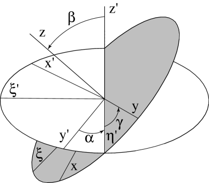
FIG. 1.: The y-convention of the Euler angles.

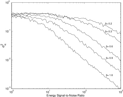
FIG. 2.: The results of a numerical simulation describing the variance of the polarization angle $\alpha$ for a range of SNR and several values of the direction angle $\beta$. Each line was computed by a 500 trial Monte Carlo simulation for 100 logarithmically spaced SNR for the corresponding value of $\beta$.

Class	Allowable polarization states	Example
$II_{6}$	$\Phi_{22}$, $\Psi_{4}$, $\Psi_{3}$, $\Psi_{2}$	Most general
$III_{5}$	$\Phi_{22}$, $\Psi_{4}$, $\Psi_{3}$	Kaluza-Klein
$N_{3}$	$\Phi_{22}$, $\Psi_{4}$	Brans-Dicke
$N_{2}$	$\Psi_{4}$	General relativity
$O_{1}$	$\Phi_{22}$	Purely scalar
$O_{0}$	None	No wave

TABLE I.: The E(2) classification scheme.