Inflation without slow roll

Abstract

We draw attention to the possibility that inflation (i.e. accelerated expansion) might continue after the end of slow roll, during a period of fast oscillations of the inflaton field $\varphi$. This phenomenon takes place when a mild non-convexity inequality is satisfied by the potential $V(\varphi)$. The presence of such a period of $\varphi$-oscillation-driven inflation can substantially modify reheating scenarios. In some models the effect of these fast oscillations might be imprinted on the primordial perturbation spectrum at cosmological scales.

The inflationary paradigm has become a widely accepted element of early universe cosmology [1, 2]. This paradigm offers the attractive possibility of resolving many of the shortcomings of standard hot big bang cosmology whilst providing an explanation for the origin of structure in the universe [3, 4, 5, 6, 7]. Although the underlying physical ideas of inflation seem well established, which concrete inflationary scenario is realized in the very early universe is unknown. There exist, at present, many inflationary scenarios, which, despite some common features, differ greatly in their details. The crucial ingredient of nearly all known successful inflationary scenarios is a period of “slow roll” evolution of the inflaton field, during which a quasi-homogeneous scalar field $\varphi$ changes very slowly, so that its kinetic energy $\dot{\varphi}^{2}/2$ during inflation remains always much smaller than its potential energy $V(\varphi)$ [8, 9, 10]. Such a period of $\varphi$-domination is well known to generate an accelerated expansion of the universe, thereby providing a natural mechanism for solving the causality and homogeneity puzzles of hot big bang cosmology. The standard inflationary lore assumes that the end of the slow roll evolution marks the end of inflation, and that it is followed by a non-inflationary period during which the inflaton $\varphi$ oscillates rapidly around the minimum of its potential $V(\varphi)$.

The main aim of this work is to draw attention to the possibility that inflation might continue after the end of slow roll, during a period of fast oscillations of $\varphi$. Such a period of $\varphi$-oscillation-driven inflation presents novel physical characteristics which can be crucial for the theory of reheating and which may modify some features of the fluctuation spectra expected from inflation. The possibility of $\varphi$-oscillation-driven inflation has (as far as we know) not been previously noticed. Most authors work mainly with the simplest renormalizable tree-level potentials, like $V(\varphi)=\frac{1}{2}\,m^{2}\,\varphi^{2}$ or $V(\varphi)=\frac{1}{4}\,\lambda\,\varphi^{4}$. For such potentials, and more generally for convex functions $V(\varphi)$ (with vanishing minimum), the end of slow roll necessarily marks the end of inflation. By contrast, we shall see that non convex functions $V(\varphi)$ can, as long as a certain inequality is satisfied, entail the continuation of inflation after the end of slow roll. Such non convex potentials might arise in various ways. Let us only mention two possibilities. First, supergravity and/or superstring physics may generate very general types of non-renormalizable potentials depending on several scalar fields $\phi_{i}$, $V(\phi_{i})=\Lambda^{4}\,{\cal V}\,(\phi_{i}/\widetilde{m}_{P})$. The inflaton $\varphi$ would then correspond to a relatively flat direction in the space of scalar fields. Second, loop-contributions to a classically $\varphi$-independent potential naturally generate a logarithmic potential for large values of $\varphi$ in some supersymmetric models [11, 12, 13, 14]: $V(\varphi)\sim A\,\ln(\varphi/\mu)+B$. When the coefficient $A$ is positive (which is the case of the models of Refs. [11, 12], except when the gauge coupling contribution dominates the scalar couplings one), such a logarithmic potential is not convex ($V_{,\varphi\varphi}<0$). However, it is not clear whether such loop-corrected potentials can sustain the type of oscillatory inflation discussed below because, when $\varphi$ becomes small the fields whose masses depend on $\varphi$ may become light or tachyonic, so that one must consider a multi-field dynamics.

In units where $\widetilde{m}_{P}=(4\pi G)^{-1/2}=1$, a conveniently redundant set of evolution equations for a scalar-driven (flat) Friedmann cosmology read

$$\ddot{\varphi}+3H\dot{\varphi}+V_{,\varphi}=0\,,$$ (1)

$$H^{2}=\frac{2}{3}\,\epsilon\,,$$ (2)

$$\dot{\epsilon}=-3H(\epsilon+p)=-3H\,\dot{\varphi}^{2}\,,$$ (3)

$$\frac{\ddot{a}}{a}=-\frac{1}{3}\,(\epsilon+3p)\,.$$ (4)

Here, $H\equiv\dot{a}/a$ is the physical-time expansion rate, $V_{,\varphi}\equiv\partial V/\partial\varphi$, $\epsilon\equiv\frac{1}{2}\,\dot{\varphi}^{2}+V(\varphi)$ denotes the energy density of the scalar field, and $p\equiv\frac{1}{2}\,\dot{\varphi}^{2}-V(\varphi)$ its pressure. Only two equations among Eqs. (1)-(4) are independent. The “slow roll” regime is the case where one can neglect $\frac{1}{2}\,\dot{\varphi}^{2}$ in $\epsilon$ and $\ddot{\varphi}$ in Eq. (1). It is easy to see that slow roll can take place only when the potential $V\left(\varphi\right)$ satisfies the following conditions: $\varepsilon_{1}\equiv\dot{\varphi}^{2}/2V\simeq\frac{1}{12}\,(V_{,\varphi}/V)^{2}\ll 1$ and $\varepsilon_{2}\equiv\ddot{\varphi}/3H\dot{\varphi}\simeq\frac{1}{6}\,V_{,\varphi\varphi}/V-\varepsilon_{1}\ll 1$. Then the effective adiabatic index of the scalar matter, $\gamma_{{\rm slow\,roll}}\equiv(\epsilon+p)/\epsilon=\dot{\varphi}^{2}/\epsilon\simeq 2\,\varepsilon_{1}$ is much smaller than one. This guarantees that the right-hand side of Eq. (4) is positive, i.e. that the expansion is accelerated.

The slow roll conditions are sufficient, but not necessary to maintain inflation. We derive below the general conditions on the potential $V\left(\varphi\right)$ under which inflation can proceed even during a stage of fast oscillations of the scalar field. For simplicity, we consider an even potential, $V(\varphi)=V(-\varphi)$, which has its minimum at $\varphi=0$. Slow roll is then followed by a stage where $\varphi$ oscillates symmetrically around 0. For generic potentials (as we shall check below), the $\varphi$-oscillations become “adiabatic” soon after the exit from slow roll (i.e. when $|\varphi|\lesssim 1$), in the sense that the expansion rate $H$ becomes much smaller than the frequency of oscillations $\omega$. In the adiabatic approximation $H\ll\omega$, one can find approximate solutions of Eqs. (1)-(4) by separating the two time scales characterizing the evolution [15] (we have also checked numerically the validity of this approximation). On the fast, oscillation time scale, one first neglects the Hubble damping terms $\propto 3H$ in Eqs. (1) and (3), and gets $\varphi$ as a function of time by inverting the integral obtained by writing the conservation of energy, $\epsilon\simeq{\rm const}=V_{m}$, where $V_{m}\equiv V(\varphi_{m})$ denotes the maximum current value of the potential energy:

$$t-t_{0}=\pm\int d\varphi\,[2(V_{m}-V(\varphi))]^{-1/2}\,.$$ (5)

The full oscillation period is

$$T\equiv 2\pi/\omega=4\int_{0}^{\varphi_{m}}d\varphi\,[2(V_{m}-V(\varphi))]^{-1/2}\,.$$ (6)

On the longer, expansion time scale, the energy $\epsilon$ is slowly drained out by the Hubble damping terms. From Eq. (3) the oscillation-averaged fractional energy loss reads

$$\langle\dot{\epsilon}/\epsilon\rangle=-3\langle H(\epsilon+p)/\epsilon\rangle\simeq-3H\gamma\,,$$ (7)

where the angular brackets denote a time average, and where $\gamma\equiv\langle(\epsilon+p)/\epsilon\rangle\equiv\langle\dot{\varphi}^{2}/\epsilon\rangle$ is the average adiabatic index of scalar matter (the averaged equation of state is $p=(\gamma-1)\,\epsilon$). From Eq. (4), one sees that the condition for inflation to continue during the $\varphi$-oscillation regime (i.e. the condition for accelerated expansion $\ddot{a}>0$) is $\gamma<\frac{2}{3}$. This condition can be rewritten in several ways in terms of the potential $V(\varphi)$. Indeed, neglecting the expansion of the universe, one easily derives the following set of equalities

$$\gamma=\frac{\langle\dot{\varphi}^{2}\rangle}{\epsilon}=\frac{\langle\varphi\,V_{,\varphi}\rangle}{V_{m}}=2\left(1-\frac{\langle V\rangle}{V_{m}}\right)=2\,\frac{\int_{0}^{1}d\widehat{\varphi}\,(1-\widehat{V})^{1/2}}{\int_{0}^{1}d\widehat{\varphi}\,(1-\widehat{V})^{-1/2}}\,,$$ (8)

where in the last one $\widehat{\varphi}\equiv\varphi/\varphi_{m}$ and $\widehat{V}\equiv V(\varphi)/V_{m}$. Using Eqs. (8), the condition $\gamma<\frac{2}{3}$ for having a $\varphi$-oscillation-driven inflation can also be written as

$$\langle V-\varphi\,V_{,\varphi}\rangle>0\,,$$ (9)

which has a very simple geometrical interpretation. Indeed, the quantity $U(\varphi)\equiv V(\varphi)-\varphi\,V_{,\varphi}\,(\varphi)$ is simply the “intercept” of the tangent to the curve $V=V(\varphi)$ at the point $\varphi$, i.e. its intersection with the vertical axis $\varphi=0$ (see Fig. 1). The condition is therefore that the time-average, over an oscillation, of the intercept $\langle U\rangle=T^{-1}\int_{0}^{T}dt\,U(\varphi(t))$ must be positive. In the case where $V_{0}=V(\varphi=0)$ is either strictly zero (as in Fig. 1) or very small compared to $V_{m}$, this geometrical interpretation shows that one needs potentials $V(\varphi)$ which are sufficiently non convex near the maximum amplitude $\varphi_{m}$ to compensate the negative $U$’s contributed by the convex part of $V(\varphi)$ near the bottom $\varphi=0$. Then inflation continues as long as $\varphi_{m}$ is larger than some value $\varphi_{c}$ defining the size of the convex core (around $\varphi=0$) of $V(\varphi)$.

Let us apply our general considerations to a simple class of potentials within which the condition (9) can be satisfied, without fine tuning, in many models. Namely, we consider potentials having at most polynomial growth when $\varphi\gg\varphi_{c}:V(\varphi)\sim\varphi^{q}$, with any (positive) real exponent $q$. In these models, slow roll takes place when $\varphi\gg 1$ and terminates around $\varphi\sim 1$. When $\varphi\ll 1$ one can use the adiabatic oscillation approximation because the “adiabaticity parameter” is seen, using equations given above, to be generically $H/\omega\sim\varphi$. To be more concrete let us take, for instance, the class of models,

$$V(\varphi)=\frac{A}{q}\,\left[\left(\frac{\varphi^{2}}{\varphi_{c}^{2}}+1\right)^{\frac{1}{2}q}-1\right]\,,$$ (10)

containing one dimensionless real parameter $q>0$, and two dimensionful parameters: an overall scale $A\sim({\rm mass})^{4}$, and the scale $\varphi_{c}$ (which could be the weak scale) determining the size of the convex core of $V(\varphi)$. In the limit $q\rightarrow 0$, this gives a logarithmic potential $V(\varphi)=\frac{1}{2}\,A\,\ln(1+\varphi^{2}/\varphi_{c}^{2})$ similar to the ones naturally arising in the supersymmetric models mentioned above. If $\varphi_{c}\ll 1$ (in Planck units), then, after the end of slow roll, one can have many oscillations with $\varphi_{m}\gg\varphi_{c}$. At $\varphi\gg\varphi_{c}$ the potential $V\left(\varphi\right)$ can be well approximated by the power law potential $V(\varphi)\simeq A\,q^{-1}(\varphi/\varphi_{c})^{q}$, or a logarithmic one $V(\varphi)\simeq A\,\ln(\varphi/\varphi_{c})$ when $q\rightarrow 0$.

For such power law potentials one easily obtains from Eqs. (8) the average adiabatic index,

$$\gamma=\frac{2q}{q+2}\,,$$ (11)

as well as the adiabatic evolution laws for the various relevant physical quantities,

$$a\propto t^{\frac{2}{3\gamma}}=t^{\frac{q+2}{3q}}\,,$$ (13)

$$\epsilon=V(\varphi_{m})\propto t^{-2}\propto a^{-\frac{6q}{q+2}}\,,$$ (14)

$$\varphi_{m}\propto t^{-\frac{2}{q}}\propto a^{-\frac{6}{q+2}}\,,$$ (15)

$$V_{,\varphi\varphi}\,(\varphi_{m})\propto t^{\frac{2(2-q)}{q}}\propto a^{6\,\frac{2-q}{2+q}}\,.$$ (16)

We note that: (i) inflation continues during the $\varphi$-oscillation-driven expansion if $\gamma<2/3$, i.e. $q<1$; (ii) the logarithmic case, $V\simeq A\,\ln(\varphi/\varphi_{c})$, interestingly leads to quasi-exponential inflation. [When $q\rightarrow 0$ Eqs. (11) and (11) get modified because $\gamma$ is not zero but only logarithmically small, $\gamma=(\ln\,(\varphi_{m}/\varphi_{c}))^{-1}$, leading, e.g., to $\epsilon=\epsilon_{0}-3A\,\ln(a/a_{0})$, $\varphi_{m}\propto a^{-3}$ and $a(t)\propto\exp\left[-\frac{1}{2}\,A(t_{{\rm end}}-t)^{2}\right]$]; (iii) the total number of $e$-folds $N$ of this new type of inflation is determined (from Eq. (15) by the hierarchy between $\varphi_{{\rm initial}}\sim\widetilde{m}_{P}$ (end of slow roll) and $\varphi_{{\rm final}}\sim\varphi_{c}$ (convex core of $V(\varphi)$):

$$N\simeq\frac{q+2}{6}\ \ln\,\left(\frac{\widetilde{m}_{P}}{\varphi_{c}}\right)\,.$$ (17)

Let us also mention that the above statements can (with some changes) be extended to the case of negative powers $-2<q<0$ in Eq. (10). This corresponds to a potential $V(\varphi)$ which climbs up to a constant when $|\varphi|\gg\varphi_{c}$ and defines a trough for $|\varphi|<\varphi_{c}$. In this case, slow roll ends when $|\varphi|<\varphi_{\rm slow\;roll}\sim\varphi_{c}^{-\frac{q}{2-q}}\ll 1$. The field $\varphi$ oscillates rapidly (on the Hubble time scale) when $\varphi_{c}\ll\varphi_{m}\ll\varphi_{\rm slow\;roll}$. Eq. (11) does not apply; $\gamma$ is power-law small, and a quasi-exponential inflation takes place during $\varphi$-oscillations.

The qualitative explanation of why, despite the fast oscillations of the scalar field, we can still have an accelerated expansion of the universe is simple. When the potential $V\left(\varphi\right)$ satisfies the condition (9), the scalar field spends a dominant fraction of each period of oscillation on the upper parts of the potential, where the kinetic energy $\dot{\varphi}^{2}/2$ is small compared to $V\left(\varphi\right)$. Therefore, the main contribution to the averaged effective equation of state comes from $V\left(\varphi\right).$

The classical estimate Eq. (17) severely constrains the total number of $e$-folds spent during any $\varphi-$oscillation-driven inflation. In the case of a logarithmic potential ($q\simeq 0$), and the extreme case of a weak-scale core $\varphi_{c}\sim 300\,{\rm Ge}V$, one gets $N\simeq 12$. This is sizable, but still small compared to the total needed duration of inflation, $N_{{\rm tot}}>65$. Moreover, if we impose some other reasonable restrictions on the model then the number of allowed $e$-folds can become even smaller. In particular, if one requires that the observable cosmological perturbations were produced during the slow roll stage of the evolution of the field $\varphi$ and that the mass of $\varphi$ near the core is smaller than the Planck mass, then $N\lesssim 5(2+q)/(2-q)$. However, even in such a case, the $\varphi$-oscillation-driven inflation can still lead to some interesting consequences which we briefly discuss below.

Up to this point we have discussed the evolution of a classical homogeneous background $\varphi(t)$, neglecting the backreaction of the quantum fluctuations of the inflaton field. However, these fluctuations can be strongly amplified because of the fast oscillations of $\varphi$ and can have a dramatic backreaction effect on the evolution of the background. Let us consider the fluctuations of the gauge-invariant variable $v=a\,[\delta\varphi^{(gi)}+(\dot{\varphi}/H)\,\Phi]$ [18] which describes the coupled scalar-matter gravity fluctuations. The mode of $v$ with comoving spatial momentum $k$ satisfies the equation (in conformal time: $v^{\prime\prime}\equiv\partial^{2}v/\partial\eta^{2}$)

$$v^{\prime\prime}+(k^{2}-U_{0}(\eta))\,v=0\,,$$ (18)

$$U_{0}=z^{\prime\prime}/z=a^{2}\,[-V_{,\varphi\varphi}-4V_{,\varphi}\,\dot{\varphi}/H-7\dot{\varphi}^{2}+2H^{2}+2\dot{\varphi}^{4}/H^{2}]\,,$$ (19)

where $z\equiv a\,\dot{\varphi}/H$. The effective potential for scalar fluctuations $U_{0}(\eta)$ exhibits novel features during the $\varphi$ oscillations associated with a non convex potential $V(\varphi)$. Indeed, the dominant term in Eq. (19) is proportional to the squared “effective” mass of the scalar field $m_{\varphi}^{2}\equiv\,V_{,\varphi\varphi}$ which is mostly  negative and oscillates with an increasing frequency and an increasing amplitude (see Eq. (16)). The resulting, mostly positive, oscillations of the effective potential $U_{0}(\eta)\simeq-a^{2}\,V_{,\varphi\varphi}$ are much more efficient at amplifying the fluctuations of $v$ than even the broadly resonant Mathieu-equation-type ones recently discussed [16]. We shall leave to future work a discussion of the effects of such a new type of super-broad resonance and only note here that the associated fast exponential growth of scalar fluctuations will quickly modify the classical, adiabatic evolution presented above, and can bring interesting new features in reheating theory. One of the simplest examples of such new features is the possibility, due to the increase of the oscillation frequency $\omega\sim(-V_{,\varphi\varphi}\,(\varphi_{m}))^{1/2}$ as $\varphi_{m}$ sinks down, to generate more and more massive particles coupled to $\varphi$, thereby alleviating the usual obstacles [17] to producing the superheavy grand-unified-theory (GUT) bosons needed in GUT baryogenesis scenarios.

This very effective parametric amplification of cosmological perturbations puts also specific imprints on the primordial perturbation spectrum. However, if the presently discussed mechanism terminates inflation, then, because of the above mentioned limits on the duration of the fast-oscillation inflationary stage, it can only influence the fluctuation spectra on small length scales. Nevertheless, it is easy to imagine how (with some amount of fine tuning) one can translate the effect of our mechanism on cosmologically relevant length scales. It suffices to consider hybrid-type inflationary models where a first bout of (slow roll, plus oscillation-driven) inflation linked to the evolution of $\varphi$ is followed by a secondary bout of inflation driven by another scalar field. With adequate tuning of the duration of the secondary inflation the effects of the $\varphi$-oscillation-driven inflation might be imprinted on cosmological scales.

We thank Andrei Linde and Antonio Riotto for useful discussions.

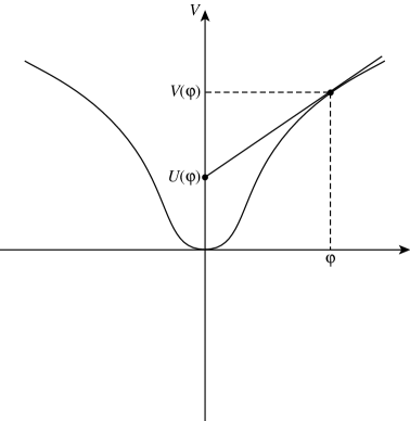
FIG. 1.: Intercept $U(\varphi)$ of the tangent to the curve $V=V(\varphi)$ at the point $\varphi$. Inflation continues after slow roll if the time-average of $U(\varphi(t))$ over one $\varphi$-oscillation is positive.

REFERENCES

- [1] A.H. Guth, Phys. Rev. D23 (1981) 347.
- [2] A. Linde, Particle Physics and Inflationary Cosmology (1990) Harwood, NJ.
- [3] V. Mukhanov and G. Chibisov. Pis’ma Zh. Eksp. Teor. Fiz. 33 (1981) 549.
- [4] A.H. Guth and S.-Y. Pi. Phys. Rev. Lett. 49 (1982) 1110.
- [5] S.W. Hawking. Phys. Lett. 115B (1982) 295.
- [6] A.A. Starobinskii. Phys. Lett. 117B (1982) 175.
- [7] J.M. Bardeen, P.J. Steinhardt, and M.S. Turner. Phys. Rev. D28 (1983) 679-693.
- [8] A. Linde, Phys. Lett. 129B (1983) 177.
- [9] A. Linde, Phys. Lett. 108B (1982) 389.
- [10] A. Albrecht, P. Steinhardt Phys. Rev. Lett. 48 (1982) 1220.
- [11] E. Witten, Phys. Lett. 105B (1981) 267.
- [12] S. Dimopoulos and S. Raby, Nucl. Phys. B219 (1983) 479.
- [13] G. Dvali, Q. Shafi and R.K. Schaefer, Phys. Rev. Lett. 73 (1994) 1886.
- [14] A. Linde and A. Riotto, Phys. Rev. D56 (1997) R1841.
- [15] M.S. Turner, Phys. Rev. D28 (1983) 1243.
- [16] L. Kofman, A. Linde and A.A. Starobinsky, Phys. Rev. Lett. 73 (1994) 3195.
- [17] E.W. Kolb, A. Linde and A. Riotto, Phys. Rev. Lett. 77 (1996) 4290.
- [18] V.F. Mukhanov, H.A. Feldman, and R.H. Brandenberger. Phys. Rep. 215 (1992) 203-333.