Chapter 1

Black Hole Perturbation

Yasushi Mino^1,2, Misao Sasaki¹, Masaru Shibata¹,

Hideyuki Tagoshi³ and Takahiro Tanaka¹

¹Department of Earth and Space Science, Osaka University, Toyonaka 560, Japan
²Department of Physics, Kyoto University, Kyoto 606, Japan
³National Astronomical Observatory, Mitaka, Tokyo 181, Japan

Abstract

In this chapter, we present analytic calculations of gravitational waves from a particle orbiting a black hole. We first review the Teukolsky formalism for dealing with the gravitational perturbation of a black hole. Then we develop a systematic method to calculate higher order post-Newtonian corrections to the gravitational waves emitted by an orbiting particle. As applications of this method, we consider orbits that are nearly circular, including exactly circular ones, slightly eccentric ones and slightly inclined orbits off the equatorial plane of a Kerr black hole and give the energy flux and angular momentum flux formulas at infinity with higher order post-Newtonian corrections. Using a different method that makes use of an analytic series representation of the solution of the Teukolsky equation, we also give a post-Newtonian expanded formula for the energy flux absorbed by a Kerr black hole for a circular orbit.

1 Introduction

In this chapter, we review recent progress in the analytic calculations of gravitational waves from a particle orbiting a black hole using a systematic post-Newtonian expansion method. There has been substantial activities in this field recently and there is a diversity of literature. Here we are mostly concerned with the actual calculations of the gravitational waves from an orbiting particle and we intend to make this chapter as self-contained as possible. We do not, however, discuss much about implications of the results to actual astrophysical situations.

In the black hole perturbation approach, one considers gravitational waves from a particle of mass $\mu$ orbiting a black hole of mass $M$ assuming $\mu\ll M$. Although this method is restricted to the case when $\mu\ll M$, one can calculate very high order post-Newtonian corrections to gravitational waves using a relatively simple algorithm in contrast with the standard post-Newtonian analysis. This is because the fully relativistic effect of the spacetime curvature is naturally taken into account in the basic perturbation equation. We can also calculate numerically the gravitational waves without assuming the slow motion of its source. Then, we can easily investigate the convergence of the post-Newtonian expansion by comparing the result of the post-Newtonian approximation with the fully relativistic one. In this sense, the black hole perturbation method gives a very important test of the post-Newtonian expansion. Further, since the effect of the spacetime curvature is naturally taken into account, we can easily investigate interesting relativistic effects such as tails of gravitational waves.

We consider the post-Newtonian wave forms and luminosity which are expanded by $v/c$, where $v$ is the order of the orbital velocity. The lowest order of the gravitational waves are given by the Newtonian quadrupole formula. We call the post-Newtonian formulas for the wave forms and luminosity which contain terms up to $O((v/c)^{n})$ beyond the Newtonian quadrapole formula as the $n/2$PN formulas.

Let us first briefly give a historical review. The gravitational perturbation equation of a black hole using the Newman-Penrose formalism[1] was derived by Bardeen and Press [2] for the Schwarzschild black hole, and by Teukolsky [3] for the Kerr black hole. By using these equations, many numerical calculations of gravitational waves induced by the presence of a test particle have been done. We do not list up all such works. Here, we only refer to three articles; Breuer[4], Chandrasekhar[5], and Nakamura, Oohara, and Kojima[6].

On the other hand, analytic calculations of gravitational waves produced by the motion of a test particle have not been developed very much until recently. This direction of research was first done by Gal’tsov, Matiukhin and Petukhov[7] in which they considered a case when a particle moves a slightly eccentric orbit around a Schwarzschild black hole, and calculated the gravitational waves up to 1PN order. Then, Poisson [8] considered a case of circular orbit around a Schwarzschild black hole and calculated the wave forms and luminosity to 1.5PN order at which the tail effect appears. Cutler, Finn, Poisson and Sussman [9] also worked on the same problem numerically by using the least square fitting method, and obtained a formula for the luminosity to 2.5PN order. Subsequently, a highly accurate numerical calculation was carried out by Tagoshi and Nakamura [10]. They obtained the formulas for the luminosity to 4PN order numerically by using the least square fitting method. They found the $\log v$ terms in the luminosity formula at 3PN and 4PN orders. They showed that, although the convergence of the post-Newtonian expansion is slow, the luminosity formula which is accurate to 3.5PN order will be good enough to represent the orbital phase evolution of coalescing compact binaries accurately. After that, Sasaki [11] found an analytic method and obtained the formulas which are needed to calculate the gravitational waves to 4PN order. Then, Tagoshi and Sasaki[12] obtained the gravitational wave forms and luminosity to 4PN order analytically, and confirmed the results of Tagoshi and Nakamura. These calculations were extended to 5.5PN order by Tanaka, Tagoshi, and Sasaki[13].

In the case of orbits around a Kerr black hole, Poisson calculated the 1.5PN order corrections to the wave forms and luminosity due to the rotation of the black hole and showed that the result agrees with the standard post-Newtonian effect due to spin-orbit coupling[14]. Then, Shibata, Sasaki, Tagoshi and Tanaka [15] calculated the luminosity to 2.5PN order. They calculated the luminosity from a particle in circular orbit with small inclination from the equatorial plane. They used the Sasaki-Nakamura equation as well as the Teukolsky equation. This analysis was extended to 4PN order by Tagoshi, Shibata, Tanaka and Sasaki [16] in which the orbit of the test particle was restricted to circular ones on the equatorial plane. The analysis in the case of slightly eccentric orbit on the equatorial plane was also done by Tagoshi [17] to 2.5PN order.

Tanaka, Mino, Sasaki, and Shibata [18] considered the case when a spinning particle moves a circular orbits near the equatorial plane around a Kerr black hole, and derived the luminosity formula to 2.5PN order including the linear order effect of the particle’s spin. They used the equations of motion of Papapetrou’s [19] and the energy momentum tensor of the spinning particle given by Dixon [20].

The absorption of gravitational waves into the black hole horizon, appearing at 4PN order in the Schwarzschild case, was calculated by Poisson and Sasaki in the case when a test particle is in a circular orbit[21]. The black hole absorption in the case of rotating black hole appears at 2.5PN order [22]. Recently a new analytic method to solve the homogeneous Teukolsky equation was found by Mano, Suzuki, and Takasugi [23]. Using this method, the black hole absorption in the case of rotating black hole was calculated by Tagoshi, Mano, and Takasugi [24] to 6.5PN order beyond the quadrupole formula.

If gravity is not described by the Einstein theory but by the Brans-Dicke theory, there will appear scalar type gravitational waves as well as transverse-traceless gravitational waves. Such scalar type gravitational waves were calculated by Ohashi, Tagoshi and Sasaki[25] in a case when a compact star is in a circular orbit on the equatorial plane around a Kerr black hole.

The organization of this chapter is as follows. We review the Teukolsky formalism for the black hole perturbation in section 2 and formulate a post-Newtonian expansion method of the Teukolsky equation in section 3. Then we turn to the evaluation of gravitational waves by an orbiting particle in the rest of sections.

First we consider circular orbits. In section 4, we calculate the gravitational wave luminosity from a test particle in circular orbit around a Schwarzschild black hole to 5.5PN order, based on Tanaka, Tagoshi, and Sasaki[13]. This is the highest post-Newtonian order achieved so far. Based on this result, we investigate the convergence property of the post-Newtonian expansion in section 5. In section 6, we consider circular orbits on the equatorial plane around a Kerr black hole and calculate the luminosity to 4PN order, based on Tagoshi, Shibata, Tanaka, and Sasaki[16]. We find the luminosity contains the terms which describe the effect of not only spin-orbit coupling but also the effect of higher multipole moments of the Kerr black hole.

Next we consider slightly noncircular orbits. In section 7, we calculate the $O(e^{2})$ corrections to the 4PN energy and angular momentum flux formulas in the case of a slightly eccentric orbit around a Schwarzschild black hole, where $e$ is the eccentricity. In section 8, we consider a slightly eccentric orbit on the equatorial plane around a Kerr black hole and evaluate the $O(e^{2})$ corrections to 2.5PN order, based on Tagoshi [17]. Then in section 9, we calculate the gravitational waves induced by a test particle in circular orbit with small inclination from the equatorial plane around a Kerr black hole and evaluate the 2.5PN energy and angular momentum fluxes, based on Shibata, Sasaki, Tagoshi, Tanaka[15]. In section 10, we discuss the adiabatic orbital evolution around a Kerr black hole under radiation reaction and show that circular orbits will remain circular under adiabatic radiation reaction but the stability of circular orbits can only be examined by an explicit evaluation of the backreaction force.

In section 11, we consider the effect of the spin of a particle. We first give a general formalism to treat the gravitational radiation from a spinning particle orbiting a Kerr black hole. Then we calculate the 2.5PN luminosity formula with the first order corrections of the spin for circular orbits which are slightly inclined due to the spin of the particle.

Finally, in section 12, we review a calculation of the black hole absorption based on Tagoshi, Mano, and Takasugi [24]. The black hole absorption effect appears at $O(v^{5})$ relative to the Newtonian quadrupole luminosity for a Kerr black hole, while at $O(v^{8})$ for a Schwarzschild black hole. We show the energy absorption rate to $O(v^{8})$ beyond the lowest order for the Kerr case, i.e., $O(v^{13})$ or 6.5PN order beyond the Newtonian quadrupole luminosity.

Since many of the calculations encountered in this black hole perturbation approach are lengthy, various subsidiary equations and formulas are deferred to appendices A to J. In the rest of this chapter, we use the units of $c=G=1$.

2 Teukolsky formalism

In terms of the conventional Boyer-Lindquist coordinates, the metric of a Kerr black hole is expressed as

$$ds^{2} = -{\mathchar 28929\relax\over\mathchar 28934\relax}(dt-a\sin^{2}\theta\,d\varphi)^{2}+{\sin^{2}\theta\over\mathchar 28934\relax}\left[(r^{2}+a^{2})d\varphi-a\,dt\right]^{2}$$ (2.1)

$$+{\mathchar 28934\relax\over\mathchar 28929\relax}dr^{2}+\mathchar 28934\relax d\theta^{2}\,,$$

where $\mathchar 28934\relax=r^{2}+a^{2}\cos^{2}\theta$ and $\mathchar 28929\relax=r^{2}-2Mr+a^{2}$. In the Teukolsky formalism[3], the gravitational perturbations of a Kerr black hole are described by a Newman-Penrose quantity $\psi_{4}=-C_{\alpha\beta\gamma\delta}n^{\alpha}\bar{m}^{\beta}n^{\gamma}\bar{m}^{\delta}$, where $C_{\alpha\beta\gamma\delta}$ is the Weyl tensor, $n^{\alpha}=((r^{2}+a^{2}),-\mathchar 28929\relax,0,a)/(2\mathchar 28934\relax)$ and $m^{\alpha}=(ia\sin\theta,0,1,i/\sin\theta)/(\sqrt{2}(r+ia\cos\theta))$.

We decompose $\psi_{4}$ into Fourier-harmonic components according to

$$(r-ia\cos\theta)^{4}\psi_{4}=\sum_{\ell m}\int d\omega e^{-i\omega t+im\varphi}\ _{-2}S_{\ell m}(\theta)R_{\ell m\omega}(r),$$ (2.2)

The radial function $R_{\ell m\omega}$ and the angular function ${}_{s}S_{\ell m}(\theta)$ satisfy the Teukolsky equations with $s=-2$ as

$$\mathchar 28929\relax^{2}{d\over dr}\left({1\over\mathchar 28929\relax}{dR_{\ell m\omega}\over dr}\right)-V(r)R_{\ell m\omega}=T_{\ell m\omega},$$ (2.3)

$$\Bigl{[}{1\over\sin\theta}{d\over d\theta}\Bigl{\{}\sin\theta{d\over d\theta}\Bigr{\}}-a^{2}\omega^{2}\sin^{2}\theta-{(m-2\cos\theta)^{2}\over\sin^{2}\theta}$$

$$~{}~{}~{}~{}~{}~{}~{}~{}~{}~{}~{}~{}~{}~{}~{}+4a\omega\cos\theta-2+2ma\omega+\lambda\Bigr{]}{}_{-2}S_{\ell m}=0.$$ (2.4)

The potential $V(r)$ is given by

$$V(r)=-{K^{2}+4i(r-M)K\over\mathchar 28929\relax}+8i\omega r+\lambda,$$ (2.5)

where $K=(r^{2}+a^{2})\omega-ma$ and $\lambda$ is the eigenvalue of ${}_{-2}S_{\ell m}^{a\omega}$. The angular function ${}_{s}S_{\ell m}(\theta)$ is the spin-weighted spheroidal harmonic which may be normalized as

$$\int_{0}^{\pi}|_{-2}S_{\ell m}|^{2}\sin\theta d\theta=1.$$ (2.6)

The source term $T_{\ell m\omega}$ is specified later. Here we only mention that for orbits of our interest, which are bounded, $T_{\ell m\omega}$ has support in a compact range of $r$.

We define two kinds of homogeneous solutions of the radial Teukolsky equation:

$$R^{\rm in}_{\ell m\omega}\to\cases{B^{\rm trans}_{\ell m\omega}\mathchar 28929\relax^{2}e^{-ikr^{*}}\,&for $r\to r_{+}$\cr r^{3}B^{\rm ref}_{\ell m\omega}e^{i\omega r^{*}}+r^{-1}B^{\rm inc}_{\ell m\omega}e^{-i\omega r^{*}}\,&for $r\to+\infty,$\cr}$$ (2.7)

$$R^{\rm up}_{\ell m\omega}\to\cases{C^{\rm up}_{\ell m\omega}e^{ikr^{*}}+\mathchar 28929\relax^{2}C^{\rm ref}_{\ell m\omega}e^{-ikr^{*}}\,&for $r\to r_{+},$\cr C^{\rm trans}_{\ell m\omega}r^{3}e^{i\omega r^{*}}\,&for $r\to+\infty$\cr}$$ (2.8)

where $k=\omega-ma/2Mr_{+}$ and $r^{*}$ is the tortoise coordinate defined by

$$r^{*} = \int{dr^{*}\over dr}dr$$ (2.9)

$$= r+{2Mr_{+}\over{r_{+}-r_{-}}}\ln{{r-r_{+}}\over 2M}-{2Mr_{-}\over{r_{+}-r_{-}}}\ln{{r-r_{-}}\over 2M},$$

where $r_{\pm}=M\pm\sqrt{M^{2}-a^{2}}$, and for definiteness, we have fixed the integration constant.

We solve the radial Teukolsky equation by using the Green function method. A solution of the Teukolsky equation which has purely outgoing property at infinity and has purely ingoing property at the horizon is given by

$$R_{\ell m\omega}={1\over W_{\ell m\omega}}\left\{R^{\rm up}_{\ell m\omega}\int^{r}_{r_{+}}dr^{\prime}R^{\rm in}_{\ell m\omega}T_{\ell m\omega}\mathchar 28929\relax^{-2}+R^{\rm in}_{\ell m\omega}\int^{\infty}_{r}dr^{\prime}R^{\rm up}_{\ell m\omega}T_{\ell m\omega}\mathchar 28929\relax^{-2}\right\},$$ (2.10)

where the Wronskian $W_{\ell m\omega}$ is given by

$$W_{\ell m\omega}=2i\omega C^{\rm trans}_{\ell m\omega}B^{\rm inc}_{\ell m\omega}.$$ (2.11)

Then, the solution has an asymptotic property at the horizon as

$$R_{\ell m\omega}(r\to r_{+})\to{{B^{\rm trans}_{\ell m\omega}\mathchar 28929\relax^{2}e^{-ikr^{*}}}\over 2i\omega C^{\rm trans}_{\ell m\omega}B^{\rm inc}_{\ell m\omega}}\int^{\infty}_{r_{+}}dr^{\prime}R^{\rm up}_{\ell m\omega}T_{\ell m\omega}\mathchar 28929\relax^{-2}\equiv\tilde{Z}^{\rm H}_{\ell m\omega}\mathchar 28929\relax^{2}e^{-ikr^{*}},$$ (2.12)

The solution at infinity is also expressed as

$$R_{\ell m\omega}(r\to\infty)\to{r^{3}e^{i\omega r^{*}}\over 2i\omega B^{\rm inc}_{\ell m\omega}}\int^{\infty}_{r_{+}}dr^{\prime}{T_{\ell m\omega}(r^{\prime})R^{\rm in}_{\ell m\omega}(r^{\prime})\over\mathchar 28929\relax^{2}(r^{\prime})}\equiv\tilde{Z}_{\ell m\omega}^{\infty}r^{3}e^{i\omega r^{*}},$$ (2.13)

Here and in the following sections except for section 12, we focus on the gravitational waves emitted to infinity. Hence $\tilde{Z}_{\ell m\omega}^{\infty}$ will be simply denoted as $\tilde{Z}_{\ell m\omega}$. The gravitational waves absorbed into the black hole horizon will be treated separately in section 12.

Now let us discuss the general form of the source term $T_{\ell m\omega}$. It is given by

$$T_{\ell m\omega}=4\int d\mathchar 28938\relax dt\rho^{-5}{\overline{\rho}}^{-1}(B_{2}^{\prime}+B_{2}^{\prime*})e^{-im\varphi+i\omega t}{{}_{-2}S^{a\omega}_{\ell m}\over\sqrt{2\pi}},$$ (2.14)

where

$$B_{2}^{\prime} = -{1\over 2}\rho^{8}{\overline{\rho}}L_{-1}[\rho^{-4}L_{0}(\rho^{-2}{\overline{\rho}}^{-1}T_{nn})]$$

$$- {1\over 2\sqrt{2}}\rho^{8}{\overline{\rho}}\mathchar 28929\relax^{2}L_{-1}[\rho^{-4}{\overline{\rho}}^{2}J_{+}(\rho^{-2}{\overline{\rho}}^{-2}\mathchar 28929\relax^{-1}T_{{\overline{m}}n})],$$

$$B_{2}^{\prime*} = -{1\over 4}\rho^{8}{\overline{\rho}}\mathchar 28929\relax^{2}J_{+}[\rho^{-4}J_{+}(\rho^{-2}{\overline{\rho}}T_{{\overline{m}}{\overline{m}}})]$$ (2.15)

$$- {1\over 2\sqrt{2}}\rho^{8}{\overline{\rho}}\mathchar 28929\relax^{2}J_{+}[\rho^{-4}{\overline{\rho}}^{2}\mathchar 28929\relax^{-1}L_{-1}(\rho^{-2}{\overline{\rho}}^{-2}T_{{\overline{m}}n})],$$

with

$$\rho = (r-ia\cos\theta)^{-1},$$

$$L_{s} = \partial_{\theta}+{m\over\sin\theta}-a\omega\sin\theta+s\cot\theta,$$ (2.16)

$$J_{+} = \partial_{r}+{iK/\mathchar 28929\relax}\,.$$

In the above, $T_{nn}$, $T_{{\overline{m}}n}$ and $T_{{\overline{m}}{\overline{m}}}$ are the tetrad components of the energy momentum tensor ($T_{nn}=T_{\mu\nu}n^{\mu}n^{\nu}$ etc.), and the bar denotes the complex conjugation.

We consider $T_{\mu\nu}$ of a monopole particle of mass $\mu$. The case of a spinning particle will be discussed in section 11 separately. The energy momentum tensor takes the form,

$$T^{\mu\nu}={\mu\over\mathchar 28934\relax\sin\theta dt/d\tau}{dz^{\mu}\over d\tau}{dz^{\nu}\over d\tau}\delta(r-r(t))\delta(\theta-\theta(t))\delta(\varphi-\varphi(t)).$$ (2.17)

where $z^{\mu}=\bigl{(}t,r(t),\theta(t),\varphi(t)\bigr{)}$ is a geodesic trajectory and $\tau=\tau(t)$ is the proper time along the geodesic. The geodesic equations in Kerr geometry are given by

$$\mathchar 28934\relax{d\theta\over d\tau}=\pm\Bigl{[}C-\cos^{2}\theta\Bigl{\{}a^{2}(1-E^{2})+{l_{z}^{2}\over\sin^{2}\theta}\Bigr{\}}\Bigr{]}^{1/2}\equiv\mathchar 28930\relax(\theta),$$

$$\mathchar 28934\relax{d\varphi\over d\tau}=-\Bigl{(}aE-{l_{z}\over\sin^{2}\theta}\Bigr{)}+{a\over\mathchar 28929\relax}\Bigl{(}E(r^{2}+a^{2})-al_{z}\Bigr{)}\equiv\mathchar 28936\relax,$$

$$\mathchar 28934\relax{dt\over d\tau}=-\Bigl{(}aE-{l_{z}\over\sin^{2}\theta}\Bigr{)}a\sin^{2}\theta+{r^{2}+a^{2}\over\mathchar 28929\relax}\Bigl{(}E(r^{2}+a^{2})-al_{z}\Bigr{)}\equiv T,$$

$$\mathchar 28934\relax{dr\over d\tau}=\pm\sqrt{R},$$ (2.18)

where $E$, $l_{z}$ and $C$ are the energy, the $z$-component of the angular momentum and the Carter constant of a test particle, respectively. $\mathchar 28934\relax=r^{2}+a^{2}\cos^{2}\theta$ and

$$R=[E(r^{2}+a^{2})-al_{z}]^{2}-\mathchar 28929\relax[(Ea-l_{z})^{2}+r^{2}+C].$$ (2.19)

Using Eq. (2.18), the tetrad components of the energy momentum tensor are expressed as

$$T_{n\,n} = \mu{C_{n\,n}\over\sin\theta}\delta(r-r(t))\delta(\theta-\theta(t))\delta(\varphi-\varphi(t)),$$

$$T_{{\overline{m}}\,n} = \mu{C_{{\overline{m}}\,n}\over\sin\theta}\delta(r-r(t))\delta(\theta-\theta(t))\delta(\varphi-\varphi(t)),$$ (2.20)

$$T_{{\overline{m}}\,{\overline{m}}} = \mu{C_{{\overline{m}}\,{\overline{m}}}\over\sin\theta}\delta(r-r(t))\delta(\theta-\theta(t))\delta(\varphi-\varphi(t)),$$

where

$$C_{n\,n} = {1\over 4\mathchar 28934\relax^{3}\dot{t}}\left[E(r^{2}+a^{2})-al_{z}+\mathchar 28934\relax{dr\over d\tau}\right]^{2},$$

$$C_{{\overline{m}}\,n} = -{\rho\over 2\sqrt{2}\mathchar 28934\relax^{2}\dot{t}}\left[E(r^{2}+a^{2})-al_{z}+\mathchar 28934\relax{dr\over d\tau}\right]\left[i\sin\theta\Bigl{(}aE-{l_{z}\over\sin^{2}\theta}\Bigr{)}\right],$$ (2.21)

$$C_{{\overline{m}}\,{\overline{m}}} = {\rho^{2}\over 2\mathchar 28934\relax\dot{t}}\left[i\sin\theta\Bigl{(}aE-{l_{z}\over\sin^{2}\theta}\Bigr{)}\right]^{2},$$

and $\dot{t}=dt/d\tau$. Substituting Eq. (2.15) into Eq. (2.14) and performing integration by part, we obtain

$$T_{\ell m\omega} = {4\mu\over\sqrt{2\pi}}\int^{\infty}_{-\infty}dt\int d\theta e^{i\omega t-im\varphi(t)}$$ (2.22)

$$\times \Bigl{[}-{1\over 2}L_{1}^{{\dagger}}\bigl{\{}\rho^{-4}L_{2}^{{\dagger}}(\rho^{3}S)\bigr{\}}C_{n\,n}\rho^{-2}{\overline{\rho}}^{-1}\delta(r-r(t))\delta(\theta-\theta(t))$$

$$+ {\mathchar 28929\relax^{2}{\overline{\rho}}^{2}\over\sqrt{2}\rho}\bigl{(}L_{2}^{{\dagger}}S+ia({\overline{\rho}}-\rho)\sin\theta S\bigr{)}J_{+}\bigl{\{}C_{{\overline{m}}\,n}\rho^{-2}{\overline{\rho}}^{-2}\mathchar 28929\relax^{-1}\delta(r-r(t))\delta(\theta-\theta(t))\bigr{\}}$$

$$+ {1\over 2\sqrt{2}}L_{2}^{{\dagger}}\bigl{\{}\rho^{3}S({\overline{\rho}}^{2}\rho^{-4})_{,r}\bigr{\}}C_{{\overline{m}}\,n}\mathchar 28929\relax\rho^{-2}{\overline{\rho}}^{-2}\delta(r-r(t))\delta(\theta-\theta(t))$$

$$- {1\over 4}\rho^{3}\mathchar 28929\relax^{2}SJ_{+}\bigl{\{}\rho^{-4}J_{+}\bigl{(}{\overline{\rho}}\rho^{-2}C_{{\overline{m}}\,{\overline{m}}}\delta(r-r(t))\delta(\theta-\theta(t))\bigr{)}\bigr{\}}\Bigr{]},$$

where

$$L_{s}^{{\dagger}}=\partial_{\theta}-{m\over\sin\theta}+a\omega\sin\theta+s\cot\theta,$$ (2.23)

and $S$ denotes ${}_{-2}S_{\ell m}^{a\omega}(\theta)$ for simplicity.

We further rewrite Eq. (2.22) as

$$T_{\ell m\omega} = \mu\int^{\infty}_{-\infty}dte^{i\omega t-im\varphi(t)}\mathchar 28929\relax^{2}\Bigl{[}(A_{n\,n\,0}+A_{{\overline{m}}\,n\,0}+A_{{\overline{m}}\,{\overline{m}}\,0})\delta(r-r(t))$$ (2.24)

$$+ \left\{(A_{{\overline{m}}\,n\,1}+A_{{\overline{m}}\,{\overline{m}}\,1})\delta(r-r(t))\right\}_{,r}+\left\{A_{{\overline{m}}\,{\overline{m}}\,2}\delta(r-r(t))\right\}_{,rr}\Bigr{]},$$

where

$$A_{n\,n\,0} = {-2\over\sqrt{2\pi}\mathchar 28929\relax^{2}}C_{n\,n}\rho^{-2}{\overline{\rho}}^{-1}L_{1}^{+}\{\rho^{-4}L_{2}^{+}(\rho^{3}S)\},$$

$$A_{{\overline{m}}\,n\,0} = {2\over\sqrt{\pi}\mathchar 28929\relax}C_{{\overline{m}}\,n}\rho^{-3}\Bigl{[}\left(L_{2}^{+}S\right)\Bigl{(}{iK\over\mathchar 28929\relax}+\rho+{\overline{\rho}}\Bigr{)}$$

$$\qquad-a\sin\theta S{K\over\mathchar 28929\relax}({\overline{\rho}}-\rho)\Bigr{]},$$

$$A_{{\overline{m}}\,{\overline{m}}\,0} = -{1\over\sqrt{2\pi}}\rho^{-3}{\overline{\rho}}C_{{\overline{m}}\,{\overline{m}}}S\Bigl{[}-i\Bigl{(}{K\over\mathchar 28929\relax}\Bigr{)}_{,r}-{K^{2}\over\mathchar 28929\relax^{2}}+2i\rho{K\over\mathchar 28929\relax}\Bigr{]},$$

$$A_{{\overline{m}}\,n\,1} = {2\over\sqrt{\pi}\mathchar 28929\relax}\rho^{-3}C_{{\overline{m}}\,n}[L_{2}^{+}S+ia\sin\theta({\overline{\rho}}-\rho)S],$$

$$A_{{\overline{m}}\,{\overline{m}}\,1} = -{2\over\sqrt{2\pi}}\rho^{-3}{\overline{\rho}}C_{{\overline{m}}\,{\overline{m}}}S\Bigl{(}i{K\over\mathchar 28929\relax}+\rho\Bigr{)},$$

$$A_{{\overline{m}}\,{\overline{m}}\,2} = -{1\over\sqrt{2\pi}}\rho^{-3}{\overline{\rho}}C_{{\overline{m}}\,{\overline{m}}}S.$$ (2.25)

Inserting Eq. (2.24) into Eq. (2.13), we obtain $\tilde{Z}_{\ell m\omega}$ as

$$\tilde{Z}_{\ell m\omega}={\mu\over 2i\omega B^{\rm inc}_{\ell m\omega}}\int^{\infty}_{-\infty}dte^{i\omega t-im\varphi(t)}W_{\ell m\omega}\,,$$ (2.26)

where

$$W_{\ell m\omega} = \Bigl{[}R^{\rm in}_{\ell m\omega}\{A_{n\,n\,0}+A_{{\overline{m}}\,n\,0}+A_{{\overline{m}}\,{\overline{m}}\,0}\}$$ (2.27)

$$-{dR^{\rm in}_{\ell m\omega}\over dr}\{A_{{\overline{m}}\,n\,1}+A_{{\overline{m}}\,{\overline{m}}\,1}\}+{d^{2}R^{\rm in}_{\ell m\omega}\over dr^{2}}A_{{\overline{m}}\,{\overline{m}}\,2}\Bigr{]}_{r=r(t)}\,.$$

In this paper, we focus on orbits which are either circular (with or without inclination) or eccentric but confined on the equatorial plane. In either case, the frequency spectrum of $T_{\ell m\omega}$ becomes discrete. Accordingly $\tilde{Z}_{\ell m\omega}$ in Eq. (2.12) or (2.13) takes the form,

$$\tilde{Z}_{\ell m\omega}=\sum_{n}\delta(\omega-\omega_{n})Z_{\ell m\omega}\,.$$ (2.28)

Then, in particular, $\psi_{4}$ at $r\to\infty$ is obtained from Eq. (2.2) as

$$\psi_{4}={1\over r}\sum_{\ell mn}Z_{\ell m\omega_{n}}{{}_{-2}S_{\ell m}^{a\omega_{n}}\over\sqrt{2\pi}}e^{i\omega_{n}(r^{*}-t)+im\varphi}.$$ (2.29)

At infinity, $\psi_{4}$ is related to the two independent modes of gravitational waves $h_{+}$ and $h_{\times}$ as

$$\psi_{4}={1\over 2}(\ddot{h}_{+}-i\ddot{h}_{\times}).$$ (2.30)

From Eqs.(2.29) and (2.30), the luminosity averaged over $t\gg\mathchar 28929\relax t$, where $\mathchar 28929\relax t$ is the characteristic time scale of the orbital motion (e.g., a period between the two consecutive apastrons), is given by

$$\left\langle{dE\over dt}\right\rangle=\sum_{\ell,m,n}{\Bigl{|}Z_{\ell m\omega_{n}}\Bigr{|}^{2}\over 4\pi\omega_{n}^{2}}\equiv\sum_{\ell,m,n}\Bigl{(}{dE\over dt}\Bigr{)}_{\ell mn}.$$ (2.31)

In the same way, the time-averaged angular momentum flux is given by

$$\left\langle{dJ_{z}\over dt}\right\rangle=\sum_{\ell,m,n}{m\Bigl{|}Z_{\ell m\omega_{n}}\Bigr{|}^{2}\over 4\pi\omega_{n}^{3}}\equiv\sum_{\ell,m,n}\Bigl{(}{dJ_{z}\over dt}\Bigr{)}_{\ell mn}=\sum_{\ell,m,n}{m\over\omega_{n}}\Bigl{(}{dE\over dt}\Bigr{)}_{\ell mn}\,.$$ (2.32)

3 Post-Newtonian expansion of the ingoing wave solutions

We consider the case when a test particle of mass $\mu$ is in an orbit which is nearly circular around a Kerr black hole of mass $M\gg\mu$ and describe a method to calculate the ingoing wave Teukolsky functions $R^{\rm in}_{\ell m\omega}$ which are necessary to evaluate the 4PN formulas for the gravitational waves energy and angular momentum fluxes emitted to infinity. In the Schwarzschild case, we shall derive the 5.5PN luminosity formula in section 4. A method to calculate the ingoing wave solutions in this case is separately discussed in Appendix D because it is considerably more complicated than the method explained in this section.

Using non-dimensional variables in the Teukolsky equation, we can see that the Teukolsky equation is expressed in terms of three basic variables, $z\equiv\omega r$, $\epsilon\equiv 2M\omega$ and $a\omega\equiv q\epsilon/2$ where $q\equiv a/M$. In order to calculate the gravitational waves induced by a particle, we need to know the explicit form of the source terms $T_{\ell m\omega}(r)$. They will be given in the proceeding sections for specified orbits. Here it is sufficient to note that they have support only around $r=r_{0}$ where $r_{0}$ is the orbital radius for a circular orbit or the mean radius in the case of an eccentric orbit (with small eccentricity). Hence from Eq. (2.13), what we need to know are the ingoing wave functions $R^{{\rm in}}(r)$ around $r=r_{0}$, and their incident amplitudes $B^{{\rm inc}}$. Note that we do not need the transmission amplitudes $B^{{\rm trans}}$ to evaluate the gravitational waves at infinity. This fact considerably simplifies the calculations. Since we treat a test particle in a bound orbit which is nearly circular, the contribution of $\omega$ to the Teukolsky functions comes from $\omega\sim m\mathchar 28938\relax_{\varphi}$, where $\mathchar 28938\relax_{\varphi}\sim(M/r_{0}^{3})^{1/2}$ is the orbital angular frequency. We will evaluate $R^{\rm in}$ by setting three basic variables to be $z=\omega r_{0}\sim m(M/r_{0})^{1/2}$ $\sim v$, $\epsilon\sim 2m(M/r_{0})^{3/2}$ $\sim v^{3}$, and $a\omega$ $\sim qm(M/r_{0})^{3/2}$ $\sim v^{3}$. Here, we have introduced a parameter $v\equiv(M/r_{0})^{1/2}$ which represents the magnitude of the orbital velocity. We assume that $v$ is much smaller than the velocity of light; $v\ll 1$. Consequently, we also assume that $\epsilon\ll v\ll 1$. This relation is the basic assumption in obtaining the homogeneous solutions below.

Now we calculate the ingoing wave solutions which are necessary to calculate the luminosity to $O(v^{8})$ beyond the lowest order for the Kerr case. The method is mainly based on Shibata et al.[15] and Tagoshi et al.[16]. An extension to $O(v^{11})$ calculations done by Tanaka, Tagoshi and Sasaki[13] for the Schwarzschild case is given in Appendix D.

First, we discuss the angular solutions. The angular solutions are the spin-weighted spheroidal harmonics. The angular equation (2.4) contains only one small parameter $a\omega$. It is straightforward to calculate the spin-weighted spheroidal harmonic ${}_{-2}S_{\ell m}$ and its eigenvalue $\lambda$ by expanding the solution in power of $a\omega$. It can be done by the usual perturbation method[26, 16, 15]. It is also possible to obtain them by using an expansion by means of Jacobi functions[27]. The method and the results are given explicitly in Appendix A. Here we only show the eigenvalue $\lambda$ which is used to calculate the radial functions. The eigenvalue $\lambda$ is given by

$$\lambda=\lambda_{0}+a\omega\lambda_{1}+a^{2}\omega^{2}\lambda_{2}+O((a\omega)^{3})$$ (3.1)

where

$$\lambda_{0}=\ell(\ell+1)-2=(\ell-1)(\ell+2),$$

$$\lambda_{1}=-2m{\ell(\ell+1)+4\over\ell(\ell+1)}\,,$$

$$\lambda_{2}=-2(\ell+1)(c_{\ell m}^{\ell+1})^{2}+2\ell(c_{\ell m}^{\ell-1})^{2}+{2\over 3}-{2\over 3}{(\ell+4)(\ell-3)(\ell^{2}+\ell-3m^{2})\over\ell(\ell+1)(2\ell+3)(2\ell-1)}\,,$$ (3.2)

with

$$c_{\ell m}^{\ell+1}={2\over(\ell+1)^{2}}\Bigl{[}{(\ell+3)(\ell-1)(\ell+m+1)(\ell-m+1)\over(2\ell+1)(2\ell+3)}\Bigr{]}^{1/2},$$

$$c_{\ell m}^{\ell-1}=-{2\over\ell^{2}}\Bigl{[}{(\ell+2)(\ell-2)(\ell+m)(\ell-m)\over(2\ell+1)(2\ell-1)}\Bigr{]}^{1/2}.$$ (3.3)

Next we consider the homogeneous solution $R^{{\rm in}}$. We assume $\omega>0$ below. The solution for $\omega<0$ can be obtained from the one for $\omega>0$ by using the symmetry of the homogeneous Teukolsky equation which implies $\overline{R_{\ell,m,\omega}}=R_{\ell,-m,-\omega}$. Here, we do not treat the Teukolsky equation directly. Instead, we transform the homogeneous Teukolsky equation to the Sasaki-Nakamura equation [28], which is given by

$$\Bigl{[}{d^{2}\over dr^{*2}}-F(r){d\over dr^{*}}-U(r)\Bigr{]}X_{\ell m\omega}=0.$$ (3.4)

The function $F(r)$ is given by

$$F(r)={\eta_{,r}\over\eta}{\mathchar 28929\relax\over r^{2}+a^{2}},$$ (3.5)

where

$$\eta=c_{0}+c_{1}/r+c_{2}/r^{2}+c_{3}/r^{3}+c_{4}/r^{4},$$ (3.6)

with

$$c_{0} =-12i\omega M+\lambda(\lambda+2)-12a\omega(a\omega-m),$$ (3.7)

$$c_{1} =8ia[3a\omega-\lambda(a\omega-m)],$$

$$c_{2} =-24iaM(a\omega-m)+12a^{2}[1-2(a\omega-m)^{2}],$$

$$c_{3} =24ia^{3}(a\omega-m)-24Ma^{2},$$

$$c_{4} =12a^{4}.$$

The function $U(r)$ is given by

$$U(r)={\mathchar 28929\relax U_{1}\over(r^{2}+a^{2})^{2}}+G^{2}+{\mathchar 28929\relax G_{,r}\over r^{2}+a^{2}}-FG,$$ (3.8)

where

$$G = -{2(r-M)\over r^{2}+a^{2}}+{r\mathchar 28929\relax\over(r^{2}+a^{2})^{2}},$$

$$U_{1} = V+{\mathchar 28929\relax^{2}\over\beta}\Bigl{[}\Bigl{(}2\alpha+{\beta_{,r}\over\mathchar 28929\relax}\Bigr{)}_{,r}-{\eta_{,r}\over\eta}\Bigl{(}\alpha+{\beta_{,r}\over\mathchar 28929\relax}\Bigr{)}\Bigr{]},$$

$$\alpha = -i{K\beta\over\mathchar 28929\relax^{2}}+3iK_{,r}+\lambda+{6\mathchar 28929\relax\over r^{2}},$$

$$\beta = 2\mathchar 28929\relax\Bigl{(}-iK+r-M-{2\mathchar 28929\relax\over r}\Bigr{)}.$$ (3.9)

When we set $a=0$, this transformation becomes the Chandrasekhar transformation [29] for the Schwarzschild black hole. The Sasaki-Nakamura equation was originally introduced, for the inhomogeneous case, to make the potential term short-ranged and to make the source term well-behaved at infinity. It is not necessary to perform this transformation in this case, since we are interested only in bound orbits. Nevertheless we choose to do this because the lowest order solution becomes the spherical Bessel function and we can apply the post-Newtonian expansion techniques developed for the Schwarzschild case by Poisson [8] and Sasaki [11].

The relation between $R_{\ell m\omega}$ and $X_{\ell m\omega}$ is

$$R_{\ell m\omega}={1\over\eta}\Bigl{\{}\Bigl{(}\alpha+{\beta_{,r}\over\mathchar 28929\relax}\Bigr{)}\chi_{\ell m\omega}-{\beta\over\mathchar 28929\relax}\chi_{\ell m\omega,r}\Bigr{\}},$$ (3.10)

where $\chi_{\ell m\omega}=X_{\ell m\omega}\mathchar 28929\relax/(r^{2}+a^{2})^{1/2}$. Conversely, we can express $X_{\ell m\omega}$ in terms of $R_{\ell m\omega}$ as

$$X_{\ell m\omega}=(r^{2}+a^{2})^{1/2}\,r^{2}\,J_{-}J_{-}\left[{1\over r^{2}}R_{\ell m\omega}\right],$$ (3.11)

where $J_{-}=(d/dr)-i(K/\mathchar 28929\relax)$. Then the asymptotic behavior of the ingoing-wave solution $X^{{\rm in}}$ which corresponds to Eq. (2.7) is

$$X^{\rm in}_{\ell m\omega}\to\cases{A^{\rm ref}_{\ell m\omega}e^{i\omega r^{*}}+A^{\rm inc}_{\ell m\omega}e^{-i\omega r^{*}}\,&for $r^{*}\to\infty$\cr A^{\rm trans}_{\ell m\omega}e^{-ikr^{*}}\,&for $r^{*}\to-\infty$.}$$ (3.12)

The coefficient $A^{\rm inc}$, $A^{\rm ref}$ and $A^{\rm trans}$ are respectively related to $B^{\rm inc}$, $B^{\rm ref}$ and $B^{\rm trans}$, defined in Eq. (2.7), by

$$B^{\rm inc}_{\ell m\omega} = -{1\over 4\omega^{2}}A^{\rm inc}_{\ell m\omega},$$ (3.13)

$$B^{\rm ref}_{\ell m\omega} = -{4\omega^{2}\over c_{0}}A^{\rm ref}_{\ell m\omega},$$ (3.14)

$$B^{\rm trans}_{\ell m\omega} = {1\over d_{\ell m\omega}}A^{\rm trans}_{\ell m\omega},$$ (3.15)

where $c_{0}$ is given in Eq. (3.7) and

$$d_{\ell m\omega} = \sqrt{2Mr_{+}}[(8-24iM\omega-16M^{2}\omega^{2})r_{+}^{2}$$

$$+(12iam-16M+16amM\omega+24iM^{2}\omega)r_{+}-4a^{2}m^{2}-12iamM+8M^{2}].$$

Now we introduce the variable $z^{*}$ as

$$z^{*} = z+\epsilon\left[{z_{+}\over{z_{+}-z_{-}}}\ln(z-z_{+})-{z_{-}\over{z_{+}-z_{-}}}\ln(z-z_{-})\right]$$ (3.17)

$$= \omega r^{*}+\epsilon\ln\epsilon\,,$$

where $z=\omega r$ and $z_{\pm}=\omega r_{\pm}$. To solve for $X^{{\rm in}}$, we set

$$X^{\rm in}_{\ell m\omega}=\sqrt{z^{2}+a^{2}\omega^{2}}\xi_{\ell m}(z)\exp\left(-i\phi(z)\right),$$ (3.18)

where

$$\phi(z) = \int dr\left({K\over\mathchar 28929\relax}-\omega\right)$$ (3.19)

$$= z^{*}-z-{\epsilon\over 2}mq{1\over{z_{+}-z_{-}}}\ln{{z-z_{+}}\over{z-z_{-}}}\,.$$

With this choice of the phase function, the ingoing wave boundary condition at horizon reduces to that $\xi_{\ell m}$ is regular and finite at $z=z_{+}$.

Inserting Eq. (3.18) into Eq. (3.4) and expanding it in powers of $\epsilon=2M\omega$, we obtain

$$L^{(0)}[\xi_{\ell m}]=\epsilon L^{(1)}[\xi_{\ell m}]+\epsilon Q^{(1)}[\xi_{\ell m}]+\epsilon^{2}Q^{(2)}[\xi_{\ell m}]+\epsilon^{3}Q^{(3)}[\xi_{\ell m}]+\epsilon^{4}Q^{(4)}[\xi_{\ell m}]+O(\epsilon^{5}),$$ (3.20)

where $L^{(0)}$, $L^{(1)}$, $Q^{(1)}$ and $Q^{(2)}$ are differential operators given by

$$L^{(0)} = {d^{2}\over dz^{2}}+{2\over z}{d\over dz}+\left(1-{\ell(\ell+1)\over z^{2}}\right),$$ (3.21)

$$L^{(1)} = {1\over z}{d^{2}\over dz^{2}}+\left({{1}\over z^{2}}+{2i\over z}\right){d\over dz}-\left({{4}\over{z^{3}}}-{i\over z^{2}}+{1\over z}\right),$$ (3.22)

$$Q^{(1)} = {{iq\lambda_{1}}\over 2z^{2}}{d\over dz}-{{4imq}\over{l(l+1)z^{3}}},$$ (3.23)

The formulas for $Q^{(2)}$, $Q^{(3)}$ and $Q^{(4)}$ are very complicated, and they are given explicitly in Appendix B. Note that, when we set $a=0$, all $Q^{(n)}$ vanish.

By expanding $\xi_{\ell m}$ in terms of $\epsilon$ as

$$\xi_{\ell m}=\sum_{n=0}^{\infty}\epsilon^{n}\xi^{(n)}_{\ell m}(z),$$ (3.24)

we obtain from Eq. (3.20) the iterative equations,

$$L^{(0)}[\xi^{(n)}_{\ell m}]=z^{-2}W^{(n)}_{\ell m}\,,$$ (3.25)

where

$$W^{(0)}_{\ell m}=0,$$ (3.26)

$$W^{(1)}_{\ell m}=z^{2}\left(L^{(1)}[\xi^{(0)}_{\ell m}]+Q^{(1)}[\xi^{(0)}_{\ell m}]\right),$$ (3.27)

$$W^{(2)}_{\ell m}=z^{2}\left(L^{(1)}[\xi^{(1)}_{\ell m}]+Q^{(1)}[\xi^{(1)}_{\ell m}]+Q^{(2)}[\xi^{(0)}_{\ell m}]\right),$$ (3.28)

$$W^{(3)}_{\ell m}=z^{2}\left(L^{(1)}[\xi^{(2)}_{\ell m}]+Q^{(1)}[\xi^{(2)}_{\ell m}]+Q^{(2)}[\xi^{(1)}_{\ell m}]+Q^{(3)}[\xi^{(0)}_{\ell m}]\right),$$ (3.29)

$$W^{(4)}_{\ell m}=z^{2}\left(L^{(1)}[\xi^{(3)}_{\ell m}]+Q^{(1)}[\xi^{(3)}_{\ell m}]+Q^{(2)}[\xi^{(2)}_{\ell m}]+Q^{(3)}[\xi^{(1)}_{\ell m}]+Q^{(4)}[\xi^{(0)}_{\ell m}]\right).$$ (3.30)

As $\epsilon=2GM\omega$ if we recover $G$, the above expansion corresponds to the post-Minkowski expansion of the vacuum Einstein equations.

The iterative equations (3.25) have been obtained by expanding Eq. (3.4) in powers of $\epsilon$ by regarding $z=\omega r$ as the independent variable. Since the horizon is at $z=z+=O(\epsilon)$, this procedure implicitly assumes that $\epsilon\ll z$. Consequently, we cannot apply the above expansion near the horizon where the ingoing wave boundary condition is to be imposed. To implement the boundary condition correctly, we have to consider a series solution of $\xi_{\ell m}$ which is valid near the horizon as well as in the range $\epsilon\ll z$ and match it to the series solution of the form (3.24). Recently this matching problem has been rigorously solved by Mano, Suzuki, and Takasugi[23] for the original Teukolsky equation. However, for our present purpose, it is sufficient to resort to a simple power-counting argument, by which it is possible to implement the boundary condition of $\xi_{\ell m}$ at the horizon to the behaviors of $\xi^{(n)}_{\ell m}$ at $z\gg\epsilon$ for $n\leq 2\ell$ (for $n\leq 2\ell+1$ in the Schwarzschild case; see Appendix D).

Since the ingoing wave boundary condition is that $\xi_{\ell m}$ is regular at horizon, if we introduce an independent variable $x:=(z-z_{+})/\epsilon$ we can expand $\xi_{\ell m}$ near the horizon as

$$\xi_{\ell m}=\sum_{n=0}^{\infty}\epsilon^{n}\xi^{\{n\}}_{\ell m}(x),$$ (3.31)

This means we have

$$\xi_{\ell m}(0)=\xi^{\{0\}}_{\ell m}(0)\sum_{n=0}^{\infty}\epsilon^{n}C_{n}\,,$$ (3.32)

where $C_{n}=\xi^{\{n\}}_{\ell m}(0)/\xi^{\{0\}}_{\ell m}(0)$. In other words, $\xi_{\ell m}(0)$ should have a well-defined limit for $\epsilon\to 0$ except for the overall normalization factor $\xi^{\{0\}}_{\ell m}(0)$. Keeping this property in mind, let us consider the boundary conditions for Eqs. (3.26) – (3.30).

The general solution to Eq. (3.26) is immediately obtained as

$$\xi^{(0)}_{\ell m}=\alpha_{\ell m}^{(0)}j_{\ell}+\beta_{\ell m}^{(0)}n_{\ell},$$ (3.33)

where $j_{\ell}$ and $n_{\ell}$ are the spherical Bessel functions. The coefficients $\alpha_{\ell m}^{(0)}$ and $\beta_{\ell m}^{(0)}$ are to be determined by the boundary condition. For convenience, we normalize the solution $X^{\rm in}$ such that the incident amplitude $A^{\rm inc}$ is of order unity. Then both $\alpha_{\ell m}^{(0)}$ and $\beta_{\ell m}^{(0)}$ must be of order unity. Since $j_{\ell}(z)\sim z^{\ell}$ and $n_{\ell}(z)\sim z^{-\ell-1}$ for $z\ll 1$, the latter is $O(\epsilon^{2\ell+1})$ larger than the former near the horizon where $z=O(\epsilon)$. Hence Eq. (3.32) implies we should set $\beta_{\ell m}^{(0)}=0$. As for the value of $\alpha_{\ell m}^{(0)}$, since it only contributes to the overall normalization of $X^{\rm in}$, we set $\alpha_{\ell m}^{(0)}=1$ for convenience.

Inspection of Eqs. (3.27) – (3.30) reveals that the solution $\xi_{\ell m}^{(n)}$ behaves as $z^{\ell-n}$ plus the homogeneous solution $\alpha_{\ell m}^{(n)}j_{\ell}+\beta_{\ell m}^{(n)}n_{\ell}$ for $z\to 0$. As for $\alpha_{\ell m}^{(n)}$ ($n\geq 1$), they simply contribute to renormalizations of $\alpha_{\ell m}^{(0)}$. Hence we put them to zero. As for $\beta^{(n)}_{\ell m}$, from the same argument as given above, we find they may become non-zero only for $n\geq 2\ell+1$. Since $\ell\geq 2$ and $\epsilon=O(v^{3})$, this implies that the near zone contribution of $n_{\ell}\sim z^{-\ell-1}$, which is $O(v^{-(2\ell+1)})$ greater than the lowest order term $j_{\ell}$, to the gravitational waves emitted to infinity may arise only at $O(v^{10})$ beyond the quadrupole order. Since the post-Newtonian corrections we shall consider for the Kerr case are those up to $O(v^{8})$, we set $\beta^{(n)}_{\ell m}=0$ and solve the iterative equations (3.25) to $O(\epsilon^{4})$ with the boundary conditions that $\xi^{(n)}_{\ell m}\sim z^{\ell-n}$ at $z\to 0$. We note that, in the Schwarzschild case which is discussed separately in Appendix D, these boundary conditions turn out to be appropriate for $n\leq 2\ell+1$; i.e., up to one power of $\epsilon$ higher than the Kerr case.

To calculate $\xi^{(n)}_{\ell m}$ for $n\geq 1$, we rewrite Eqs. (3.27) – (3.30) in the indefinite integral form by using the spherical Bessel functions as

$$\xi^{(n)}_{\ell m}=n_{\ell}\int^{z}dzj_{\ell}W^{(n)}_{\ell m}-j_{\ell}\int^{z}dzn_{\ell}W^{(n)}_{\ell m}\,.$$ (3.34)

The calculation is straightforward but tedious. All the formulas which are needed to calculate the above integration to obtain $\xi^{(n)}_{\ell m}$ for $n\leq 2$ are shown in Appendix of Sasaki[11]. They are recapitulated in an alternative way in Appendix D. Using those formulas, we have for $n=1$,

$$\xi^{(1)}_{\ell m} = {(\ell-1)(\ell+3)\over 2(\ell+1)(2\ell+1)}j_{\ell+1}-\left({\ell^{2}-4\over 2\ell(2\ell+1)}+{2\ell-1\over\ell(\ell-1)}\right)j_{\ell-1}$$

$$~{}+R_{\ell,0}j_{0}+\sum_{m=1}^{\ell-2}\left({1\over m}+{1\over m+1}\right)R_{\ell,m}j_{m}-2D_{\ell}^{nj}+ij_{\ell}\ln z$$

$$+ {imq\over 2}\left({\ell^{2}+4}\over\ell^{2}(2\ell+1)\right)j_{\ell-1}+{imq\over 2}\left({(\ell+1)^{2}+4}\over{(\ell+1)^{2}(2\ell+1)}\right)j_{\ell+1},$$ (3.36)

where $D_{\ell}^{nj}$ is an extension of the spherical Bessel function defined in subsection D.2.1 of Appendix D;

$$D_{\ell}^{nj}={1\over 2}\left[j_{\ell}{\rm Si}(2z)-n_{\ell}\left({\rm Ci}(2z)-\gamma-\ln 2z\right)\right],$$ (3.37)

where $\gamma=0.5772\cdots$ is the Euler constant, ${\rm Ci}(x)=-\int^{\infty}_{x}dt\cos t/t$ and ${{\rm Si}(x)}=\int^{x}_{0}dt\sin t/t$, and $R_{m,k}$ is a polynomial of the inverse power of $z$ defined by

$$R_{m,k} = z^{2}(n_{m}j_{k}-j_{m}n_{k})$$ (3.38)

$$= -\sum_{r=0}^{[(m-k-1)/2]}(-1)^{r}{(m-k-1-r)!~{}\mathchar 28928\relax\left(m+{1\over 2}-r\right)\over r!~{}(m-k-1-2r)!~{}\mathchar 28928\relax\left(k+{3\over 2}+r\right)}\left({2\over z}\right)^{m-k-1-2r},$$ (3.39)

for $m>k$ and it is defined by

$$R_{m,k}=-R_{k,m}.$$ (3.40)

for $m<k$.

Next we consider $\xi^{(2)}_{\ell m}$. From Eqs.(3.34) and (3.36), we obtain $\xi^{(2)}_{\ell m}$ as

$$\xi^{(2)}_{\ell m}=f^{(2)}_{\ell}+ig^{(2)}_{\ell}+k^{(2)}_{\ell m}(q)\,,$$ (3.41)

where $f^{(2)}_{\ell}$ and $g^{(2)}_{\ell}$ are the real and imaginary parts of $\xi^{(2)}_{\ell m}$ in the Schwarzschild limit, respectively, and $k^{(2)}_{\ell m}(q)$ is the correction term due to non-vanishing $q=a/M$. For $\ell=2$ and $\ell=3$, $f^{(2)}_{\ell}$ are given by

$$f^{(2)}_{2} = -{389\over 70z^{2}}j_{0}-{113\over 420z}j_{1}+{1\over 7z}j_{3}+4D_{2}^{nnj}$$ (3.44)

$$-{5\over 3z}D_{2}^{nj}+{10\over 3}D_{1}^{nj}+{6\over z}D^{nj}_{0}+{107\over 105}D^{nj}_{-3}$$

$$-{107\over 210}j_{2}\ln z-{1\over 2}j_{2}(\ln z)^{2}\,,$$

$$f^{(2)}_{3} = {1\over 4z}j_{4}+{323\over 49z}j_{2}-{5065\over 294z^{2}}j_{1}-\left({1031\over 588z}+{445\over 14z^{3}}\right)j_{0}+{65\over 6z^{2}}n_{0}-{65\over 6z}n_{1}$$ (3.47)

$$-{3\over z}D^{nj}_{3}+{13\over 3}D^{nj}_{2}+{9\over z}D^{nj}_{1}+{30\over z^{2}}D^{nj}_{0}-{13\over 21}D^{nj}_{-4}$$

$$+4D_{3}^{nnj}-{13\over 42}j_{3}\ln z-{1\over 2}j_{3}(\ln z)^{2}\,,$$

where $D_{\ell}^{nnj}$ is defined in Appendix D, Eq. (D.35). As explained in subsection D.1 of Appendix D, the term $g^{(2)}_{\ell}$ is given for any $\ell$ as

$$g^{(2)}_{\ell}=-{1\over z}j_{\ell}+f^{(1)}_{\ell}\ln z.$$ (3.48)

The term $k^{(2)}_{\ell m}(q)$ is given for $\ell=2$ and $\ell=3$ by

$$k^{(2)}_{2m} = {{191\,i}\over{180}}\,m\,q\,j_{0}-{{{m^{2}}\,{q^{2}}\,j_{0}}\over{30}}-{{m\,q\,j_{1}}\over{10}}$$ (3.49)

$$-{{68\,i}\over{63}}\,m\,qj_{2}-{{{q^{2}}}\over{392}}j_{2}-{{73\,{m^{2}}\,{q^{2}}}\over{1764}}\,j_{2}+{{7\,m\,q\,j_{3}}\over{180}}-{i\over{72}}\,{q^{2}}\,j_{3}+{i\over{324}}\,{m^{2}}\,{q^{2}}\,j_{3}$$

$$+{{11\,i}\over{420}}\,m\,q\,j_{4}-{{{q^{2}}\,j_{4}}\over{392}}-{{71\,{m^{2}}\,{q^{2}}\,j_{4}}\over{8820}}+{{13\,i}\over 6}\,m\,q\,n_{1}$$

$$+mq\left(-{{j_{1}}\over 5}-{{13\,j_{3}}\over{90}}\right)\,\ln z+imq\left({{-2}\over 5}\,D_{1}^{nj}-{{13}\over{45}}\,D_{3}^{nj}\right),$$

$$k^{(2)}_{3m} = {{3527\,i}\over{840}}\,m\,q\,j_{1}-{{2\,{m^{2}}\,{q^{2}}\,j_{1}}\over{315}}-{{m\,q\,j_{2}}\over{36}}-{{5\,i}\over{504}}\,{q^{2}}\,j_{2}+{{5\,i}\over{2268}}\,{m^{2}}\,{q^{2}}\,j_{2}$$ (3.50)

$$-{{379\,i}\over{360}}\,m\,q\,j_{3}-{{{q^{2}}\,j_{3}}\over{360}}-{{7\,{m^{2}}\,{q^{2}}\,j_{3}}\over{720}}+{{3\,m\,q\,j_{4}}\over{160}}-{i\over{140}}\,{q^{2}}\,j_{4}+{i\over{1120}}\,{m^{2}}\,{q^{2}}\,j_{4}$$

$$+{{97\,i}\over{5040}}\,m\,q\,j_{5}-{{{q^{2}}\,j_{5}}\over{360}}-{{17\,{m^{2}}\,{q^{2}}\,j_{5}}\over{5040}}-{{103\,i}\over{48}}\,m\,q\,n_{0}+{{25\,i}\over 8}\,m\,q\,n_{2}$$

$$-\left({{13\,m\,q\,j_{2}}\over{126}}+{{5\,m\,q\,j_{4}}\over{56}}\right)\,\ln z+imq\left({{-13}\over{63}}\,D_{2}^{nj}-{{5}\over{28}}\,D_{4}^{nj}\right).$$

As noted previously, the source term $T_{\ell m\omega}$ has support only around $r=r_{0}$, hence around $z=\omega r_{0}=O(v)$. Therefore, to evaluate the source integral, we only need $X^{\rm in}$ at $z=O(v)\ll 1$, apart from the value of the incident amplitude $A^{{\rm inc}}$. Hence the post-Newtonian expansion of $X^{\rm in}$ corresponds to the expansion not only in terms of $\epsilon=O(v^{3})$, but also of $z$ by assuming $\epsilon\ll z\ll 1$. In order to evaluate the gravitational wave luminosity to $O(v^{8})$ beyond the leading order, we must calculate the series expansion of $\xi^{(n)}_{\ell m}$ in powers of $z$ for $n\leq 6-\ell$ for each $2\leq\ell\leq 6$. This follows from a simple power counting. The leading order contribution of the $\ell$-th pole is $O(v^{2(\ell-2)})$ smaller than that of the quadrupole, while the $n$-th post-Minkowski terms are $O(\epsilon^{n}z^{-n})=O(v^{2n})$ relative to the lowest order terms in the near-zone. Hence the leading term of $\xi^{(n)}_{\ell m}$ contributes at $O(v^{2(\ell-2)+2n})$ and $O(v^{8})$ is attained for $\ell+n=6$ (see Appendix C of Ref. ?).

To evaluate $A^{{\rm inc}}$, we need to know the asymptotic behavior of $\xi^{(n)}_{\ell m}$ at infinity. Since the accuracy of $A^{{\rm inc}}$ we need is $O(\epsilon^{2})$, we do not have to calculate $\xi^{(3)}_{\ell m}$ and $\xi^{(4)}_{\ell m}$ in closed analytic form. We need only the series expansion formulas for $\xi^{(3)}_{\ell m}$ and $\xi^{(4)}_{\ell m}$ around $z=0$, which are easily obtained from Eq. (3.34). This is also true for $\xi^{(2)}_{4m}$ for $\ell=4$. Inserting $\xi^{(n)}_{\ell m}$ into Eq. (3.18) and expanding it by $z$ and $\epsilon$ assuming $\epsilon\ll z\ll 1$, we obtain

$$\xi^{(3)}_{2m} = {{{-{q^{2}}}\over{30z}}-{i\over{30z}}\,m\,{q^{3}}}+{{-i}\over{30}}+{{7\,m\,q}\over{180}}-{i\over{60}}\,{m^{2}}\,{q^{2}}+{{m\,{q^{3}}}\over{36}}-{{{m^{3}}\,{q^{3}}}\over{90}}$$ (3.51)

$$-{{m\,q\,\ln z}\over{30}}-{i\over{30}}\,{m^{2}}\,{q^{2}}\,\ln z$$

$$+z\,\left({{319}\over{6300}}+{{100637\,i}\over{441000}}\,m\,q-{{{q^{2}}}\over{180}}+{{17\,{m^{2}}\,{q^{2}}}\over{1134}}+{{83\,i}\over{5880}}\,m\,{q^{3}}\right.$$

$$\left.-{{61\,i}\over{13230}}\,{m^{3}}\,{q^{3}}+{{\ln z}\over{15}}-{{106\,i}\over{1575}}\,m\,q\,\ln z-{i\over{30}}\,m\,q\,{{(\ln z)}^{2}}\right)$$

$$+O(z^{2}),$$

$$\xi^{(4)}_{2m} = {{{q^{4}}}\over{80\,{z^{2}}}}+O(z^{-1}),$$ (3.52)

$$\xi^{(3)}_{3m} = {{-i}\over{1260}}\,m\,q+{{{m^{2}}\,{q^{2}}}\over{1890}}-{i\over{1260}}\,m\,{q^{3}}-{i\over{3780}}\,{m^{3}}\,{q^{3}}+O(z),$$ (3.53)

$$\xi^{(2)}_{4m} = \Bigl{(}{1\over{1764}}-{{11\,i}\over{15120}}\,m\,q+{{{q^{2}}}\over{10584}}-{{19\,{m^{2}}\,{q^{2}}}\over{105840}}\Bigr{)}\,{z^{2}}+O(z^{3}).$$ (3.54)

Inserting these $\xi^{(n)}_{\ell m}$ into Eq. (3.18) and expanding the result in terms of $\epsilon=2M\omega$, we obtain the post-Newtonian expansion of $X^{{\rm in}}$. The transformation from $X^{{\rm in}}$ to $R^{{\rm in}}$ is done by using Eq. (3.10).

Next, we consider $A^{{\rm inc}}$ to $O(\epsilon^{2})$. Using the relation $j_{\ell+1}\sim$ $-j_{\ell-1}\sim$ $(-1)^{\ell+n}n_{2n-\ell}$ at $z\sim\infty$, etc., we obtain the asymptotic behaviors of $\xi^{(1)}_{\ell m}$ and $\xi^{(2)}_{\ell m}$ at $z\sim\infty$ as

$$\xi^{(1)}_{\ell m} \sim p^{(1)}_{\ell m}j_{\ell}+(q^{(1)}_{\ell m}-\ln z)n_{\ell}+ij_{\ell}\ln z,$$ (3.55)

$$\xi^{(2)}_{\ell m} \sim \left(p^{(2)}_{\ell m}+q^{(1)}_{\ell m}\ln z-(\ln z)^{2}\right)j_{\ell}+(q^{(2)}_{\ell m}-p^{(1)}_{\ell m}\ln z)n_{\ell}$$ (3.56)

$$+ip^{(1)}_{\ell m}j_{\ell}\ln z+i(q^{(1)}_{\ell m}-\ln z)n_{\ell}\ln z$$

where

$$p^{(1)}_{\ell m} = -{\pi\over 2},$$ (3.57)

$$q^{(1)}_{\ell m} = {1\over 2}\left[\psi(\ell)+\psi(\ell+1)+{{(\ell-1)(\ell+3)}\over\ell(\ell+1)}\right]-\ln 2-{{2imq}\over{\ell^{2}(\ell+1)^{2}}}\,,$$ (3.58)

$$\psi(\ell) = \sum^{\ell-1}_{k=1}{1\over k}-\gamma,$$ (3.59)

for any $\ell$ and

$$p^{(2)}_{2m} = {{457\,\gamma}\over{210}}-{{{{\gamma}^{2}}}\over 2}+{{5\,{{\pi}^{2}}}\over{24}}-{i\over{18}}\,\gamma\,m\,q+{{457\,\ln 2}\over{210}}$$ (3.60)

$$-\gamma\,\ln 2-{i\over{18}}\,m\,q\,\ln 2-{{{({\ln 2})^{2}}}\over 2},$$

$$q^{(2)}_{2m} = {{-457\,\pi}\over{420}}+{{\gamma\,\pi}\over 2}+{{5\,m\,q}\over{36}}+{i\over{36}}\,m\,\pi\,q-{i\over{72}}\,{q^{2}}+{i\over{324}}\,{m^{2}}\,{q^{2}}+{{\pi\,\ln 2}\over 2},$$ (3.61)

$$p^{(2)}_{3m} = {{52\,\gamma}\over{21}}-{{{{\gamma}^{2}}}\over 2}+{{5\,{{\pi}^{2}}}\over{24}}-{i\over{72}}\,\gamma\,m\,q+{{52\,\ln 2}\over{21}}$$ (3.62)

$$-\gamma\,\ln 2-{i\over{72}}\,m\,q\,\ln 2-{{{({\ln 2})^{2}}}\over 2},$$

$$q^{(2)}_{3m} = {{-26\,\pi}\over{21}}+{{\gamma\,\pi}\over 2}+{{67\,m\,q}\over{1440}}+{i\over{144}}\,m\,\pi\,q+{i\over{360}}\,{q^{2}}-{{17\,i}\over{12960}}\,{m^{2}}\,{q^{2}}+{{\pi\,\ln 2}\over 2}.$$ (3.63)

Then noting that $\exp(-i\phi)\sim\exp(-i(z^{*}-z))$ at $z\sim\infty$, the asymptotic form of $X^{\rm in}$ is expressed as

$$X^{\rm in} = \sqrt{z^{2}+a^{2}\omega^{2}}\exp(-i\phi)\left\{f^{(0)}_{\ell m}+\epsilon\xi^{(1)}_{\ell m}+\epsilon^{2}\xi^{(2)}_{\ell m}+...\right\}$$ (3.64)

$$\sim e^{-iz^{*}}(zh_{\ell}^{(2)}e^{iz})\left[1+\epsilon(p^{(1)}_{\ell m}+iq^{(1)}_{\ell m})+\epsilon^{2}(p^{(2)}_{\ell m}+iq^{(2)}_{\ell m})\right]$$

$$+e^{iz^{*}}(zh_{\ell}^{(1)}e^{-iz})\left[1+\epsilon(p^{(1)}_{\ell m}-iq^{(1)}_{\ell m})+\epsilon^{2}(p^{(2)}_{\ell m}-iq^{(2)}_{\ell m})\right],$$

where $h^{(1)}_{\ell}$ and $h^{(2)}_{\ell}$ are the spherical Hankel functions of the first and second kinds, respectively, which are given by

$$h^{(1)}_{\ell}=j_{\ell}+in_{\ell}\to(-1)^{\ell+1}{e^{iz}\over z},~{}h^{(2)}_{\ell}=j_{\ell}-in_{\ell}\to(-1)^{\ell+1}{e^{-iz}\over z}.$$ (3.65)

From these equations, noting $\omega r^{*}=z^{*}-\epsilon\ln\epsilon$, we obtain

$$A^{{\rm inc}}={1\over 2}i^{\ell+1}e^{-i\epsilon\ln\epsilon}\left[1+\epsilon(p^{(1)}_{\ell m}+iq^{(1)}_{\ell m})+\epsilon^{2}(p^{(2)}_{\ell m}+iq^{(2)}_{\ell m})+...\right].$$ (3.66)

The corresponding incident amplitude $B^{{\rm inc}}$ for the Teukolsky function is obtained from Eq. (3.13).

4 Gravitational waves to $O(v^{11})$ in Schwarzschild case

In this section we consider a circular orbit around a Schwarzschild black hole and derive the 5.5PN formula for the energy flux emitted to infinity. In this case, we can take the orbit to lie on the equatorial plane ($\theta=\pi/2$) without loss of generality. Then $E$ and $l_{z}$ are given by setting $R(r_{0})=\partial R/\partial r(r_{0})=0$ where $R$ is given by Eq. (2.19). This gives

$$E=(r_{0}-2M)/\sqrt{r_{0}(r_{0}-3M)},\quad l_{z}=\sqrt{Mr_{0}}/\sqrt{1-3M/r_{0}},$$ (4.1)

where $r_{0}$ is the orbital radius. The angular frequency is given by $\mathchar 28938\relax_{\varphi}=(M/r_{0}^{3})^{1/2}$.

Defining ${}_{s}b_{\ell m}$ by

$${}_{0}b_{\ell m} = {1\over 2}\left[(\ell-1)\ell(\ell+1)(\ell+2)\right]^{1/2}{}_{0}Y_{\ell m}\left({\pi\over 2},0\right){Er_{0}\over r_{0}-2M}\,,$$ (4.2)

$${}_{-1}b_{\ell m} = \left[(\ell-1)(\ell+2)\right]^{1/2}{}_{-1}Y_{\ell m}\left({\pi\over 2},0\right){l_{z}\over r_{0}}\,,$$ (4.3)

$${}_{-2}b_{\ell m} = {}_{-2}Y_{\ell m}\left({\pi\over 2},0\right)l_{z}\mathchar 28938\relax_{\varphi},$$ (4.4)

where ${}_{s}Y_{\ell m}(\theta,\varphi)$ are the spin-weighted spherical harmonics[30], $\tilde{Z}_{\ell m\omega}$ is found to take the form

$$\tilde{Z}_{\ell m\omega}=Z_{\ell m}\delta(\omega-m\mathchar 28938\relax_{\varphi}),$$ (4.5)

where

$$Z_{\ell m} = {\pi\over i\omega r_{0}^{2}B_{\ell\omega}^{in}}\Biggl{\{}\Biggl{[}-_{0}b_{\ell m}-2i_{-1}b_{\ell m}\left(1+{i\over 2}\omega r_{0}^{2}/(r_{0}-2M)\right)$$ (4.9)

$$+i_{-2}b_{\ell m}\omega r_{0}(1-2M/r_{0})^{-2}\left(1-M/r_{0}+{1\over 2}i\omega r_{0}\right)\Biggr{]}R_{\ell m}^{in}$$

$$+\left[i_{-1}b_{\ell m}-_{-2}b_{\ell m}\left(1+i\omega r_{0}^{2}/(r_{0}-2M)\right)\right]r_{0}{R^{in}_{\ell\omega}}^{\prime}(r_{0})$$

$$+{1\over 2}{}_{-2}b_{\ell m}r_{0}^{2}{R_{\ell\omega}^{in}}^{\prime\prime}(r_{0})\Biggr{\}}\quad,$$

where prime denotes the derivative with respect to the radial coordinate $r$. In terms of the amplitudes $Z_{\ell m}$, the gravitational wave luminosity at infinity is given by

$${dE\over dt}=\sum_{\ell=2}^{\infty}\sum_{m=-\ell}^{\ell}{|Z_{\ell m}|^{2}\over 2\pi\omega^{2}},$$ (4.10)

where $\omega=m\mathchar 28938\relax_{\varphi}$. Since the dominant frequency of the gravitational waves at infinity is $2\mathchar 28938\relax_{\varphi}$, an observationally relevant post-Newtonian parameter is $x\equiv(M\mathchar 28938\relax_{\varphi})^{1/3}$. We mention that our post-Newtonian expansion parameter is defined by $v:=(M/r_{0})^{1/2}$. In the case of a circular orbit around a Schwarzschild black hole, however, we have $v=x$. Hence the parameter $v$ is directly related to the observable frequency in the present case.

Following the method given in section 3, instead of directly calculating $R^{\rm in}_{\ell\omega}$ from the homogeneous Teukolsky equation, we calculate the corresponding Regge-Wheeler function $X^{\rm in}_{\ell\omega}$ first and then transform it to $R^{\rm in}_{\ell\omega}$. The homogeneous Regge-Wheeler equation, which is given by setting $a=0$ in Eq. (3.4), takes the form [31],

$$\left[{{d^{2}\over dr^{*2}}+\omega^{2}-V(r)}\right]X_{\ell\omega}(r)=0,$$ (4.11)

where

$$V(r)=\left({1-{2M\over r}}\right)\left({{\ell(\ell+1)\over r^{2}}-{6M\over r^{3}}}\right).$$ (4.12)

The transformation (3.10) reduces to [32]

$$R_{\ell m\omega}={\mathchar 28929\relax\over c_{0}}\left({{d\over dr^{*}}+i\omega}\right){r^{2}\over\mathchar 28929\relax}\left({{d\over dr^{*}}+i\omega}\right)rX_{\ell\omega},$$ (4.13)

where $c_{0}$, defined in Eq. (3.7), reduces to $c_{0}=(\ell-1)\ell(\ell+1)(\ell+2)-12iM\omega$. The inverse transformation (3.11) reduces to

$$X_{\ell\omega}={r^{5}\over\mathchar 28929\relax}\left({d\over dr^{*}}-i\omega\right){r^{2}\over\mathchar 28929\relax}\left({d\over dr^{*}}-i\omega\right){R_{\ell\omega}\over r^{2}}.$$ (4.14)

The asymptotic forms of $X^{\rm in}$ is the same as given in Eq. (3.12) except that now we have $k=\omega$. The coefficients $A^{\rm inc}$, $A^{\rm ref}$ and $A^{\rm trans}$ are also respectively related to $B^{\rm inc}$, $B^{\rm ref}$ and $B^{\rm trans}$ as before. (See Eqs. (3.13), (3.14) and (3.15).) Note that the coefficient that appears in Eq. (3.15) now reduces to

$$d_{\ell m\omega}=16(1-2iM\omega)(1-4iM\omega).$$ (4.15)

Corresponding to Eq. (3.17), we introduce the variable $z^{*}=z+\epsilon\ln(z-\epsilon)$. Then Eq. (3.18) reduces to

$$X_{\ell}^{\rm in}=e^{-i(z^{*}-z)}z\xi_{\ell}(z)=e^{-i\epsilon\ln(z-\epsilon)}z\xi_{\ell}(z),$$ (4.16)

and Eq. (3.20) becomes $L^{(0)}[\xi_{\ell}]=\epsilon L^{(1)}[\xi_{\ell}]$. Thus Eq. (3.25) simplifies considerably to become

$$L^{(0)}[\xi_{\ell}^{(n)}]=L^{(1)}[\xi_{\ell}^{(n-1)}].$$ (4.17)

It may be worthwhile to note that the left hand side can be expressed concisely as

$$L^{(1)}[\xi_{\ell}^{(n-1)}]=e^{-iz}{d\over dz}\left[{1\over z^{3}}{d\over dz}\left(e^{iz}z^{2}\xi_{\ell}^{(n-1)}\right)\right].$$ (4.18)

The calculations to $O(\epsilon^{2})$ are already done in section 3. When we consider the gravitational wave luminosity to $O(v^{11})$, we need to calculate $A^{\rm inc}$ to $O(\epsilon^{3})$ for $\ell=2$ and $3$ and to $O(\epsilon^{2})$ and for $\ell=4$. Thus we need the closed analytic forms of $\xi^{(3)}_{\ell}$ for $\ell=2$ and 3 and $\xi^{(2)}_{4}$. The latter can be obtained in the same way as in the previous section. The procedure to obtain $\xi^{(3)}_{\ell}$ is explained in detail in Appendix D.

The real parts of $\xi^{(3)}_{\ell}$, $f^{(3)}_{\ell}$, for $\ell=2$ and 3 are given as

$$f_{2}^{(3)}= {{214\,{F_{2,0}[z(\ln z)j_{0}]}}\over{105}}-{{107\,D^{nj}_{-4}}\over{630}}-{{457\,D^{nj}_{-2}}\over{70}}-{{2629\,D^{nj}_{0}}\over{630}}+{16949\,D^{nj}_{2}\over{4410}}$$ (4.22)

$$-{{107\,(\ln z)\,D^{nj}_{2}}\over{105}}+{(\ln z)^{2}}\,D^{nj}_{2}-{{2\,D^{nj}_{4}}\over{49}}-12\,D^{nnj}_{-1}-18\,D^{nnj}_{1}+{{2\,D^{nnj}_{3}}\over 3}$$

$$-8\,D^{nnnj}_{2}-{{197\,j_{-3}}\over{126}}+{{2539\,j_{-1}}\over{3780}}+{{107\,(\ln z)\,j_{-1}}\over{70}}+{{3\,{{(\ln z)}^{2}}\,j_{-1}}\over 2}+{{21\,j_{1}}\over{100}}$$

$$+{{349\,(\ln z)\,j_{1}}\over{140}}+{{9\,{{(\ln z)}^{2}}\,j_{1}}\over 4}-{{457\,j_{3}}\over{1050}}+{{29\,(\ln z)\,j_{3}}\over{252}}-{{{{(\ln z)}^{2}}\,j_{3}}\over{12}}+{{j_{5}}\over{504}}\,,$$

$$f_{3}^{(3)}= {{26\,F_{3,0}[z(\log z)j_{0}]}\over{21}}+{{13\,D^{nj}_{-5}}\over{98}}+{{14075\,D^{nj}_{-3}}\over{882}}$$ (4.28)

$$-{{1424\,D^{nj}_{-1}}\over{63}}-{{2511\,D^{nj}_{1}}\over{70}}+{{269\,D^{nj}_{3}}\over{70}}-{{13\,(\log z)\,D^{nj}_{3}}\over{21}}$$

$$+{{(\log z)}^{2}}\,D^{nj}_{3}-{{D^{nj}_{5}}\over{18}}+60\,D^{nnj}_{-2}+34\,D^{nnj}_{0}-{{710\,D^{nnj}_{2}}\over{21}}+{{6\,D^{nnj}_{4}}\over 7}$$

$$-8\,D^{nnnj}_{3}+{{75\,j_{-4}}\over{28}}-{{19\,j_{-2}}\over{56}}-{{65\,(\log z)\,j_{-2}}\over{14}}-{{15\,{{(\log z)}^{2}}\,j_{-2}}\over 2}-{{2789\,j_{0}}\over{3780}}$$

$$-{{221\,(\log z)\,j_{0}}\over{84}}-{{17\,{{(\log z)}^{2}}\,j_{0}}\over 4}-{{7495\,j_{2}}\over{5292}}+{{4867\,(\log z)\,j_{2}}\over{1764}}$$

$$+{{355\,{{(\log z)}^{2}}\,j_{2}}\over{84}}-{{10963\,j_{4}}\over{32340}}+{{15\,(\log z)\,j_{4}}\over{196}}-{{3\,{{(\log z)}^{2}}\,j_{4}}\over{28}}+{{4\,j_{6}}\over{1485}}\,,$$

where the definitions of the functions $D^{nnj}_{\ell}$ etc. are given in Eqs. (D.35) and (D.39) of Appendix D. The imaginary parts $g^{(3)}_{\ell}$ are expressed in terms of $f^{(1)}_{\ell}$ and $f^{(2)}_{\ell}$ as given in Eq. (D.14). As for the real part of $\xi^{(2)}_{4}$, $f^{(2)}_{4}$, it is calculated to be

$$f^{(2)}_{4} = {56\over 165\,z}j_{5}+\left(-{{5036}\over{33\,{z^{4}}}}+{30334\over 1155\,z^{2}}\right)j_{4}+\left({35252\over 33\,z^{5}}-{30334\over 165\,z^{3}}+{14401\over 3465\,z}\right)j_{3}$$ (4.32)

$$-\left({5036\over 11\,z^{5}}+{{45461}\over{693\,{z^{3}}}}+{{36287}\over{9240\,z}}\right)j_{1}+\left({{140}\over{{z^{3}}}}-{{5}\over{18\,z}}\right)n_{0}-{{49}\over{6\,z}}n_{2}$$

$$-{21\over 5\,z}D^{nj}_{4}+{149\over 30}D^{nj}_{3}-{10\over 3\,z}D^{nj}_{2}+{105\over\,z^{2}}D^{nj}_{1}+{210\over z^{3}}D^{nj}_{0}-{20\over z}D^{nj}_{0}+{1571\over 3465}D^{nj}_{-5}$$

$$+4D^{nnj}_{4}-{1571\over 6930}\,j_{4}\,\ln z-{1\over 2}\,j_{4}\,(\ln z)^{2}\,.$$

Using the analysis given in subsection D.4.2 of Appendix D, the above results readily give us the asymptotic forms of $\xi^{(3)}_{\ell}$ ($\ell=2,3$) and $\xi^{(2)}_{4}$ at $z\to\infty$, from which the amplitudes $A^{\rm inc}$ to the required order are calculated. The results are

$$A^{\rm inc}_{2} = -{1\over 2}ie^{-i\epsilon(\ln 2\epsilon+\gamma)}\exp\left[i\left\{\epsilon{5\over 3}-\epsilon^{2}{107\over 420}\pi+\epsilon^{3}\left({29\over 648}-{107\over 1260}\pi^{2}+{\zeta(3)\over 3}\right)+\cdots\right\}\right]$$ (4.35)

$$\times\Biggl{[}1-\epsilon{\pi\over 2}+\epsilon^{2}\left({25\over 18}+{5\over 24}\pi^{2}+{107\over 210}(\gamma+\ln 2)\right)$$

$$\quad+\epsilon^{3}\left(-{25\over 36}\pi-{107\over 420}(\gamma+\ln 2)\pi-{\pi^{3}\over 16}\right)+\cdots\Biggr{]},$$

$$A^{\rm inc}_{3} = {1\over 2}e^{-i\epsilon(\ln 2\epsilon+\gamma)}\exp\left[i\left\{\epsilon{13\over 6}-\epsilon^{2}{13\over 84}\pi+\epsilon^{3}\left(-{29\over 810}-{13\over 252}\pi^{2}+{\zeta(3)\over 3}\right)+\cdots\right\}\right]$$ (4.38)

$$\times\Biggl{[}1-\epsilon{\pi\over 2}+\epsilon^{2}\left({169\over 72}+{5\over 24}\pi^{2}+{13\over 42}(\gamma+\ln 2)\right)$$

$$\quad+\epsilon^{3}\left(-{169\over 144}\pi-{13\over 84}(\gamma+\ln 2)\pi-{\pi^{3}\over 16}\right)+\cdots\Biggr{]},$$

$$A^{\rm inc}_{4} = {1\over 2}ie^{-i\epsilon(\ln 2\epsilon+\gamma)}\exp\left[i\left\{\epsilon{149\over 60}-i\epsilon^{2}{1571\over 13860}\pi+\cdots\right\}\right]$$ (4.40)

$$\times\left[1-\epsilon{\pi\over 2}+\epsilon^{2}\left({22201\over 7200}+{5\over 24}\pi^{2}+{1571\over 6930}(\gamma+\ln 2)\right)+\cdots\right].$$

The corresponding amplitudes $B^{\rm inc}$ are readily obtained from Eq. (3.13).

As in the previous section, from Eqs. (4.16) and (4.13), it is also straightforward to obtain the near-zone post-Newtonian expansion of $X^{\rm in}$ and hence of $R^{\rm in}$, assuming $z\ll 1$. As discussed there, we need the series expansion formulas for $R^{\rm in}$ for $2(n+\ell-2)\leq 11$, hence for $n\leq 7-\ell$ for each $2\leq\ell\leq 7$. The resulting $R^{\rm in}$ for $2\leq\ell\leq 7$ which are necessary to calculate the luminosity to $O(v^{11})$ are given in Appendix E.

Finally, from Eq. (4.10), we obtain the luminosity to $O(v^{11})$ as

$$\left\langle{dE\over dt}\right\rangle=\left({dE\over dt}\right)_{N} \Biggl{[}1-{1247\over 336}\,v^{2}+4\,\pi\,{v^{3}}-{44711\over 9072}\,{v^{4}}-{8191\,\pi\over 672}\,{v^{5}}$$ (4.41)

$$+\left({{6643739519}\over{69854400}}-{{1712\,\gamma}\over{105}}+{{16\,{{\pi}^{2}}}\over 3}-{{3424\,\ln 2}\over{105}}-{{1712\,\ln v}\over{105}}\right)\,{v^{6}}$$

$$-{16285\,\pi\over{504}}\,{v^{7}}$$

$$+\left(-{{323105549467}\over{3178375200}}+{{232597\,\gamma}\over{4410}}-{{1369\,{{\pi}^{2}}}\over{126}}\right.$$

$$\qquad\left.+{{39931\,\ln 2}\over{294}}-{{47385\,\ln 3}\over{1568}}+{{232597\,\ln v}\over{4410}}\right)\,{v^{8}}$$

$$+\left({{265978667519\,\pi}\over{745113600}}-{{6848\,{\gamma}\,\pi}\over{105}}-{{13696\,\pi\,\ln 2}\over{105}}-{{6848\,\pi\,{\ln v}}\over{105}}\right)v^{9}$$

$$+\left(-{{2500861660823683}\over{2831932303200}}+{{916628467\,{\gamma}}\over{7858620}}-{{424223\,{{\pi}^{2}}}\over{6804}}\right.$$

$$\qquad\left.-{{83217611\,\ln 2}\over{1122660}}+{{47385\,\ln 3}\over{196}}+{{916628467\,{\ln v}}\over{7858620}}\right)v^{10}$$

$$+\left({{8399309750401\,\pi}\over{101708006400}}+{{177293\,{\gamma}\,\pi}\over{1176}}\right.$$

$$\qquad\left.+{{8521283\,\pi\,\ln 2}\over{17640}}-{{142155\,\pi\,\ln 3}\over{784}}+{{177293\,\pi\,{\ln v}}\over{1176}}\right)v^{11}\Biggr{]},$$

where $(dE/dt)_{N}$ is the Newtonian quadrupole luminosity given by

$$\left({dE\over dt}\right)_{\rm N}={32\mu^{2}M^{3}\over 5r_{0}^{5}}={32\over 5}\left({\mu\over M}\right)^{2}v^{10}.$$ (4.42)

To compare the above result with those obtained previously by the standard post-Newtonian method, we note that $v=x\equiv(M\mathchar 28938\relax_{\varphi})^{1/3}$ in the present case. Then we find our result agrees with the standard post-Newtonian results up to $O(x^{5})$[33, 34, 35, 36, 37, 38] in the limit $\mu/M$ $\ll 1$. The contributions to the luminosity from individual $\ell$ modes are given in Appendix E.

5 Convergence of the post-Newtonian expansion

Using the results obtained in the previous section, we compare the formula for the gravitational wave flux with the corresponding numerical results and investigate the accuracy of the post-Newtonian expansion.

A high precision numerical calculation of gravitational waves from a particle in a circular orbit around a Schwarzschild black hole has been performed by Tagoshi and Nakamura. [10] Since no assumption was made about the velocity of the test particle, their results are correct relativistically in the limit $\mu\ll M$. In that work, $dE/dt$ was calculated only for $\ell=2\sim 6$. Here, for the orbital radius $r_{0}\leq 100M$, we calculate $dE/dt$ again for all modes of $\ell=2\sim 6$ and for $\ell=7$ with odd $m$. The estimated accuracy of the calculation is about $10^{-11}$, which turns out to be accurate enough for the present purpose. As for the radius $r_{0}>100M$, we use the data calculated by Tagoshi and Nakamura [10] which contain modes from $\ell=2$ to $6$.

In Figs. 1 and 2, we show the error in the post-Newtonian formulas as a function of the orbital radius $r$. The error of the post-Newtonian formula is defined as

$${\rm error}=\left|1-\left(dE\over dt\right)_{n}{\hbox{$\left/\vbox to0.0pt{}\right.\n@space$}}\left(dE\over dt\right)\right|,$$ (5.1)

where $(dE/dt)_{n}$ and $(dE/dt)$ denote the $(n/2)$PN formula and the numerical result, respectively.

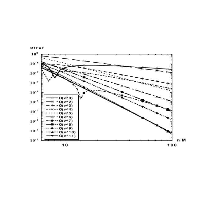
Fig. 1: The error of the post-Newtonian formulas as functions of the Schwarzschild radial coordinate $r$ for $6\leq r/M\leq 100$. Contributions from $\ell=2$ to $7$ modes are included.

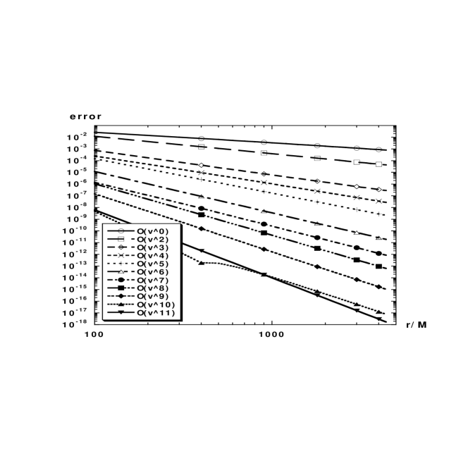
Fig. 2: The same figure for $100\leq r/M$ $<5000$. Contributions only from $\ell=2$ to $6$ are included in both the post-Newtonian formulas and in the numerical data.

In the plot of Fig.2, only the contributions from $\ell=2$ to $6$ are included in both the post-Newtonian formulas and the numerical data. We can see that, at small radius less than $r\sim 10M$, the error of the 1PN and 2.5PN formulas are larger than the other formulas. On the other hand, the Newtonian and the 2PN formulas are very accurate within this radius. This is because those formulas coincide with the exact one accidentally at a radius between $6M$ and $10M$. The error of each post-Newtonian formula at the inner most stable circular orbit, $r=6M$, becomes as follows; $12\%$ (Newtonian), $66\%$ (1PN), $8.6\%$ (1.5PN), $3.4\%$ (2PN), $42\%$ (2.5PN), $11\%$ (3PN), $5.4\%$ (3.5PN), $17\%$ (4PN), $8.4\%$ (4.5PN), $6.5\%$ (5PN), $4.1\%$ (5.5PN). As is expected, the errors of the post-Newtonian formulas decrease almost linearly up to $r\sim 5000M$ in a log-log plot. This fact also suggests that the numerical data have accuracy of at least $\sim 10^{-18}$ at $r\sim 5000M$.

In order to examine exactly to what order the post-Newtonian formulas are needed to do accurate estimation of the parameters of a binary, using data from laser interferometers, we must evaluate the systematic error produced by incorrect templates. However, here we simply calculate the total cycle of gravitational waves from a coalescing binary in a laser interferometer band and evaluate the error produced by the post-Newtonian formulas. It has been suggested that whether the error in the total cycle is less than unity or not gives a useful guideline to examine the accuracy of the post-Newtonian formulas as templates [39] (see also Ref. ?).

We ignore the finite mass effect in the post-Newtonian formulas and interpret $M$ as the total mass and $\mu$ as the reduced mass of the system. The total cycle $N$ of gravitational waves from an inspiraling binary is calculated by using the post-Newtonian energy loss formula, $(dE/dt)_{n}$, and the orbital energy formula $(dE/dv)_{n}$ which is truncated at $n/2$PN order as

$$N^{(n)}=\int^{v_{i}}_{v_{f}}dv{\mathchar 28938\relax_{\varphi}\over\pi}{(dE/dv)_{n}\over|(dE/dt)_{n}|},$$ (5.2)

where $v_{i}=(M/r_{i})^{1/2}$, $v_{f}=(M/r_{f})^{1/2}$, and $r_{i}$ and $r_{f}$ are the initial and final orbital separations of the binary. We define the relative difference of cycle $\mathchar 28929\relax N^{(n)}$ as $\mathchar 28929\relax N^{(n)}\equiv$ $|N^{(n)}-N^{(n-1)}|$. We adopt $r_{f}=6M$ and $r_{i}$ is the one at which the frequency of wave is 10Hz and which is given by $r_{i}/M\sim 347(M_{\odot}/M)^{2/3}$.

The results for typical binary systems are given in Table I.

Table I: The relative difference of cycle $\mathchar 28929\relax N^{(n)}$ for typical coalescing compact binaries. The last line shows the cycle calculated by Newtonian quadrupole formula.

$n$	(1.4$M_{\odot}$,1.4$M_{\odot}$)	(10$M_{\odot}$,10$M_{\odot}$)	(1.4$M_{\odot}$,10$M_{\odot}$)	(1.4$M_{\odot}$,70$M_{\odot}$)
2	356	54	216	212
3	228	60	208	296
4	11	5	15	31
5	12	7	20	53
6	11	8	22	75
7	1.2	1.0	2.6	10
8	0.12	0.14	0.3	2.2
9	0.82	0.80	1.9	8.9
10	0.09	0.08	0.20	0.87
11	0.03	0.03	0.07	0.40
$N^{(0)}$	16000	600	3578	898

We only show the results for $q=0$. The cases for $q\neq 0$ are investigated in Shibata et al.[15] and Tagoshi et al.[16]. This table suggests that we need the 3PN$\sim$4PN formula to obtain accurate wave forms for typical binaries whose total mass are less than 20$M_{\odot}$. Although the required post-Newtonian order is very high and it has not been achieved yet in the standard post-Newtonian analysis, this results show that the post-Newtonian approximation is applicable to the inspiral phase of coalescing compact binaries. In this sense, we can be optimistic.

On the other hand, the convergence for the case of neutron star $-$ black hole binaries, whose mass is above several ten $M_{\odot}$, is very slow. This is because $r_{i}/M$ become smaller for a larger mass black hole, and the higher relativistic correction becomes more important. From Table I, we might think that $N^{(n)}$ converges at $n=11$ even for $(m_{1},m_{2})=$ (1.4$M_{\odot}$,70$M_{\odot}$). However this is not true. Note that Table I shows only the relative difference between the post-Newtonian approximated cycles. If we calculate the difference between the post-Newtonian formula and the fully relativistic one, we find that the 5.5PN formula is not accurate enough for the case $(m_{1},m_{2})=$ (1.4$M_{\odot}$,70$M_{\odot}$), as pointed out by Tanaka, Tagoshi and Sasaki[13].

Finally we comment on the initial frequency. The above results are obtained by setting the initial frequency to 10Hz. However, it may be difficult to observe gravitational wave at this frequency because of the seismic noise. If we set the initial frequency higher than 10Hz, the error $\mathchar 28929\relax N$ becomes slightly smaller. But since this dependence of $\mathchar 28929\relax N$ on the initial frequency is very weak, the above results are insensitive to the variation of the initial frequency.

6 Circular orbit on the equatorial plane around a rotating black hole

In this section, we consider a circular orbit on the equatorial plane of a Kerr black hole and calculate the 4PN luminosity formula.

We define the orbital radius as $r=r_{0}$. As in section 4, we have $C=0$, and $E$ and $l_{z}$ are determined by $R(r_{0})=0$ and $\partial R/\partial r\mid_{r=r_{0}}=0$ as

$$E={{1-2v^{2}+qv^{3}}\over(1-3v^{2}+2qv^{3})^{1/2}}\,,\quad l_{z}={{r_{0}v(1-2qv^{3}+q^{2}v^{4})}\over(1-3v^{2}+2qv^{3})^{1/2}}\,,$$ (6.1)

where $v=(M/r_{0})^{1/2}$. From these, we can easily obtain $\varphi(t)$ as

$$\varphi(t)=\mathchar 28938\relax_{\varphi}\,t\,;\quad\mathchar 28938\relax_{\varphi}={M^{1/2}\over r_{0}^{3/2}}\left[1-qv^{3}+q^{2}v^{6}+O(v^{9})\right]\,.$$ (6.2)

When $a=0$, this becomes $\mathchar 28938\relax_{\varphi}=(M/r_{0}^{3})^{1/2}$.

The rest of the calculation is almost the same as in section 4. The amplitude of the Teukolsky function $\tilde{Z}^{\infty}_{\ell m\omega}$ at infinity is expressed as

$$\tilde{Z}^{\infty}_{\ell m\omega} = \mu{{2\pi\delta(\omega-m\mathchar 28938\relax)}\over{2i\omega B^{{\rm inc}}}}\Bigl{[}R^{{\rm in}}\{A_{n\,n\,0}+A_{{\bar{m}}\,n\,0}+A_{{\bar{m}}\,{\bar{m}}\,0}\}$$ (6.3)

$$-{dR^{{\rm in}}\over dr}\{A_{{\bar{m}}\,n\,1}+A_{{\bar{m}}\,{\bar{m}}\,1}\}+{d^{2}R^{{\rm in}}\over dr^{2}}A_{{\bar{m}}\,{\bar{m}}\,2}\Bigr{]}_{r=r_{0},\theta=\pi/2},$$

$$\equiv \delta(\omega-m\mathchar 28938\relax)Z^{\infty}_{\ell m\omega}\,,$$

where $A_{nn0}$, etc. are given by Eq. (2.25).

The total luminosity up to $O(v^{8})$ is expressed as

$$\left\langle{dE\over dt}\right\rangle=\left({dE\over dt}\right)_{\rm N} \left\{1+\left(\hbox{$q$-independent terms}\right)-{73\,q\over 12}\,{v^{3}}++{{33\,{q^{2}}}\over{16}}\,{v^{4}}\right.$$ (6.4)

$$+ {{3749\,q}\over{336}}\,{v^{5}}-\left({{169\,\pi\,q}\over 6}+{{3419\,{q^{2}}}\over{168}}\right)\,{v^{6}}$$

$$+ \left({{83819\,q}\over{1296}}+{{65\,\pi\,{q^{2}}}\over 8}-{{151\,{q^{3}}}\over{12}}\right)\,{v^{7}}$$

$$+ \left.\left({{3389\,\pi\,q}\over{96}}-{{124091\,{q^{2}}}\over{9072}}{{17\,{q^{4}}}\over{16}}\right)\,{v^{8}}\right\}\,,$$

where $(dE/dt)_{\rm N}$ is the Newtonian quadrupole luminosity, Eq. (4.42), and the $q$-independent terms are identical to those in Eq. (4.41).

From an observational point of view, it is more convenient to express the luminosity in terms of the variable $x\equiv(M\mathchar 28938\relax_{\varphi})^{1/3}$. Using the relation between $v\equiv(M/r_{0})^{1/2}$ and $x$ given by Eq. (6.2), the luminosity is expresses as

$$\left\langle{dE\over dt}\right\rangle=\widetilde{\left({dE\over dt}\right)}_{\rm N} \left(1+\left(\hbox{$q$-independent terms}\right)-{{11\,q}\over 4}\,{x^{3}}+{{33\,{q^{2}}}\over{16}}\,{x^{4}}\right.$$ (6.5)

$$- {{59\,q}\over{16}}\,{x^{5}}+\left(-{{65\,\pi\,q}\over 6}+{{611\,{q^{2}}}\over{504}}\right)\,{x^{6}}$$

$$+ \left({{162035\,q}\over{3888}}+{{65\,\pi\,{q^{2}}}\over 8}-{{71\,{q^{3}}}\over{24}}\right)\,{x^{7}}$$

$$+ \left.\left({{359\,\pi\,q}\over{14}}+{{22667\,{q^{2}}}\over{4536}}+{{17\,{q^{4}}}\over{16}}\right)\,{x^{8}}\right),$$

where

$$\widetilde{\left({dE\over dt}\right)}_{\rm N}={32\over 5}\left(\mu\over M\right)^{2}x^{10}\,,$$ (6.6)

and the $q$-independent terms are again identical to those in Eq. (4.41) with the replacement $v\to x$. The partial luminosities for individual modes are given in Appendix F. The spin dependent term at $O(v^{3})$ agrees with the standard post-Newtonian result[41].

Here it is interesting to investigate the origin of some of the spin-dependent terms. As an example, we consider the mode $\ell=|m|=2$. The luminosity from the $\ell=|m|=2$ modes is given by

$$\left({dE\over dt}\right)_{2,2}+\left({dE\over dt}\right)_{2,-2}$$ (6.7)

$$=\widetilde{\left({dE\over dt}\right)}_{\rm N} \Biggl{[}1+\left(\hbox{$q$-independent terms}\right)-{{8\,q}\over 3}\,{x^{3}}+2\,{q^{2}}\,{x^{4}}$$ (6.8)

$$+ {{52\,q}\over{27}}\,{x^{5}}+\left(-{{32\,\pi\,q}\over 3}-{{1817\,{q^{2}}}\over{567}}\right)\,{x^{6}}$$

$$+ \left({{364856\,q}\over{11907}}+8\,\pi\,{q^{2}}-{8\,q^{3}\over 3}\right)\,{x^{7}}$$

$$+ \left({{208\,\pi\,q}\over{27}}+{{105022\,{q^{2}}}\over{9261}}+{q^{4}}\right)\,{x^{8}}\Biggr{]}.$$

We can derive some of the spin-dependent terms in the above formula from the quadrupole formula [42]; $dE/dt=(32/5)\mu^{2}\hat{r}^{4}\mathchar 28938\relax_{\varphi}^{6}$, where $\hat{r}$ is the orbital radius of a test particle in harmonic coordinates. If multipole moments of the black hole exist, the orbital radius changes due to the influence of those moments. The mass and mass current multipole moments of a Kerr black hole is given by $M_{l}+iS_{l}$ $=M(ia)^{l}$. We can express the orbital frequency of the test particle in harmonic coordinates. We find that the dominant effect of the multipole moments of a Kerr black hole to $dE/dt$ can be expressed as

$$\left\langle{dE\over dt}\right\rangle=\widetilde{\left({dE\over dt}\right)}_{\rm N}\Bigl{\{} 1-{8\over 3}{S_{1}\over M^{2}}x^{3}-2{M_{2}\over M^{3}}x^{4}+\left(4{S_{3}\over M^{4}}-{4\over 3}{M_{2}S_{1}\over M^{5}}\right)x^{7}$$ (6.10)

$$+\left(-{3\over 2}{M_{2}^{2}\over M^{6}}+{5\over 2}{M_{4}\over M^{5}}\right)x^{8}\Bigr{\}}\,.$$

The terms in this expression agree with the corresponding terms of our result such as $(-8/3)qx^{3}$, $2q^{2}x^{4}$, $(-8/3)q^{3}x^{7}$ and $q^{4}x^{8}$. Thus, we may interpret the term $2q^{2}x^{4}$ as the effect of the quadrupole moment. The terms $(-8/3)q^{3}x^{7}$ and $q^{4}x^{8}$ are not due to a single multipole moment, but to combined effects of the multipole moments.

7 Slightly eccentric orbit around a Schwarzschild black hole

In this section, we present post-Newtonian formulas of gravitational waves from a particle in slightly eccentric orbits around a Schwarzschild black hole. We derive the 4PN formulas of the energy and angular momentum fluxes to $O(e^{2})$ where $e$ is the eccentricity of the orbit.

The solution of the geodesic equations for slightly eccentric orbits has been given by Apostolatos et al.[43]. Here we briefly sketch the derivation of it. Since we may consider the orbit to lie on the equatorial plane without loss of generality, we put $\theta=\pi/2$ and $C=0$ in the geodesic equations (2.18). Then we define a slightly eccentric orbit as follows: First of all, we assume that $E$ and $l_{z}$ are set to be such that $R(r)/r^{4}$, which plays the role of an effective potential for the radial motion, has the minimum at $r=r_{0}$ and that the maximum value of the orbital radius is at $r=r_{0}(1+e)$, where $e\ll 1$. Thus, the following conditions hold;

$${\partial(R/r^{4})\over\partial r}(r=r_{0})=0\quad{\rm and}\quad R(r=r_{0}(1+e))=0.$$ (7.1)

From these equations, $E$ and $l_{z}$ are expressed in terms of $r_{0}$ and $e$ as

$$E^{2}={(1-2v^{2})^{2}\over 1-3v^{2}}+{v^{2}(1-6v^{2})\over 1-3v^{2}}e^{2}-{2v^{2}(1-7v^{2})\over 1-3v^{2}}e^{3}+O(e^{4}),$$ (7.2)

$$l_{z}={M\over v\sqrt{1-3v^{2}}},$$ (7.3)

where $v\equiv\sqrt{M/r_{0}}$. For convenience, we also define $\mathchar 28938\relax\equiv v^{3}/M$. Then expanding the geodesic equations in powers of $e$, the solution is found to be[43]

$$r(t)=r_{0}[1+e\cos\mathchar 28938\relax_{r}t$$

$$\hskip 28.45274pt+e^{2}\{q_{1}(v)(1-\cos\mathchar 28938\relax_{r}t)+q_{2}(v)(1-\cos 2\mathchar 28938\relax_{r}t)\}]+O(e^{3}),$$ (7.4)

$$\varphi(t)=\mathchar 28938\relax_{\varphi}t-ep_{1}(v)\sin\mathchar 28938\relax_{r}t$$

$$\hskip 28.45274pt+e^{2}\{p_{2}(v)\sin\mathchar 28938\relax_{r}t+p_{3}(v)\sin 2\mathchar 28938\relax_{r}t\}+O(e^{3}),$$ (7.5)

where

$$\mathchar 28938\relax_{r}=\mathchar 28938\relax(1-6v^{2})^{1/2},$$ (7.6)

$$\mathchar 28938\relax_{\varphi}=\mathchar 28938\relax[1-f(v)e^{2}]~{};\quad f(v)={3(1-3v^{2})(1-8v^{2})\over 2(1-2v^{2})(1-6v^{2})},$$ (7.7)

$$q_{1}(v)={1-7v^{2}\over 1-6v^{2}},~{}~{}~{}q_{2}(v)={1-11v^{2}+26v^{4}\over 2(1-6v^{2})(1-2v^{2})},$$ (7.8)

$$p_{1}(v)={2(1-3v^{2})\over(1-2v^{2})\sqrt{1-6v^{2}}},~{}~{}~{}p_{2}(v)={2(1-3v^{2})(1-7v^{2})\over(1-2v^{2})(1-6v^{2})^{3/2}},$$

$$p_{3}(v)={5-64v^{2}+250v^{4}-300v^{6}\over 4(1-2v^{2})^{2}(1-6v^{2})^{3/2}}.$$ (7.9)

As is well known, since $\mathchar 28938\relax_{r}\neq\mathchar 28938\relax_{\varphi}$, the orbit does not close.

Now we evaluate the source term of the Teukolsky equation. In the present case, $A_{n\,n\,0}$ etc. given in Eqs. (2.25) reduce to

$$A_{n\,n\,0}=-{E\over 2\sqrt{2}\mathchar 28929\relax}S^{(0)}_{\ell m}\biggl{(}1+{r^{2}\over\mathchar 28929\relax}{dr\over dt}\biggr{)}^{2},$$ (7.10)

$$A_{\bar{m}\,n\,0}={il_{z}\over\sqrt{2\pi}}S^{(1)}_{\ell m}\biggl{(}{i\omega\over\mathchar 28929\relax}+{2\over r^{3}}\biggr{)}\biggl{(}1+{r^{2}\over\mathchar 28929\relax}{dr\over dt}\biggr{)},$$ (7.11)

$$A_{\bar{m}\,\bar{m}\,0}={l_{z}^{2}\over 2\sqrt{2\pi}E}S^{(2)}_{\ell m}\biggl{(}{2i\omega(r-M)\over\mathchar 28929\relax r^{2}}-{\omega^{2}\over\mathchar 28929\relax}\biggr{)},$$ (7.12)

$$A_{\bar{m}\,n\,1}={il_{z}\over\sqrt{2\pi}r^{2}}S^{(1)}_{\ell m}\biggl{(}1+{r^{2}\over\mathchar 28929\relax}{dr\over dt}\biggr{)},$$ (7.13)

$$A_{\bar{m}\,\bar{m}\,1}={l_{z}^{2}\over\sqrt{2\pi}E}S^{(2)}_{\ell m}\biggl{(}{i\omega\over r^{2}}+{\mathchar 28929\relax\over r^{5}}\biggr{)},$$ (7.14)

$$A_{\bar{m}\,\bar{m}\,2}={l_{z}^{2}\mathchar 28929\relax\over 2\sqrt{2\pi}Er^{4}}S^{(2)}_{\ell m}\,,$$ (7.15)

where

$$S^{(0)}_{\ell m}=L_{1}^{\dagger}L_{2}^{\dagger}S_{\ell m}({\theta=\pi/2}),$$ (7.16)

$$S^{(1)}_{\ell m}=L_{2}^{\dagger}S_{\ell m}({\theta=\pi/2}),$$ (7.17)

$$S^{(2)}_{\ell m}=S_{\ell m}({\theta=\pi/2}).$$ (7.18)

Then noting that the orbits of our interest have the properties,

$$r(t+\mathchar 28929\relax t_{r})=r(t),\qquad\left.{d\varphi\over dt}\right|_{t=t+\mathchar 28929\relax t_{r}}=\left.{d\varphi\over dt}\right|_{t=t},$$ (7.19)

where $\mathchar 28929\relax t_{r}=2\pi/\mathchar 28938\relax_{r}$, Eq. (2.26) can be rewritten as

$$\tilde{Z}_{\ell m\omega} = {\mu\over 2i\omega B^{\rm inc}_{\ell m\omega}}\int^{\infty}_{-\infty}dte^{i\omega t-im\varphi(t)}W_{\ell m\omega}$$ (7.20)

$$= {\mu\over 2i\omega B^{\rm inc}_{\ell m\omega}}{2\pi\over{\mathchar 28929\relax t_{r}}}\int^{\mathchar 28929\relax t_{r}}_{0}dte^{i\omega t-im\varphi(t)}W_{\ell m\omega}\sum_{n}\delta(\omega-\omega_{n}),$$

where

$$\omega_{n}=n\mathchar 28938\relax_{r}+m\mathchar 28938\relax_{\varphi}\quad(n=0,\pm 1,\pm 2,\ldots).$$ (7.21)

We see that $\tilde{Z}_{\ell m\omega}$ takes the form as given in Eq. (2.28) with $Z_{\ell m\omega}$ given by

$$Z_{\ell m\omega}={\mu\mathchar 28938\relax_{r}\over 2i\omega B^{\rm inc}_{\ell m\omega}}\int^{\mathchar 28929\relax t_{r}}_{0}dte^{i\omega t-im\varphi(t)}W_{\ell m\omega}\,.$$ (7.22)

When $Z_{\ell m\omega_{n}}$ are obtained, the energy and angular momentum fluxes averaged over $t\gg\mathchar 28929\relax t_{r}$ are calculated by using Eqs. (2.31) and (2.32), respectively. Here, we show these fluxes accurate to $O(e^{2})$ and to $O(v^{8})$ beyond Newtonian:

$$\left\langle{dE\over dt}\right\rangle=\dot{E}^{(0)}+e^{2}\dot{E}^{(2)}+O(e^{3}),$$ (7.23)

$$\left\langle{dJ_{z}\over dt}\right\rangle=\dot{J}^{(0)}_{z}+e^{2}\dot{J}^{(2)}_{z}+O(e^{3}).$$ (7.24)

We note that $\dot{J}^{(0)}_{z}=\dot{E}^{(0)}/\mathchar 28938\relax$ where $\mathchar 28938\relax=v^{3}/M$. We have already given the 5.5PN formula for $\dot{E}^{(0)}$ in section 4, Eq. (4.41). Hence our task here is to evaluate the $O(e^{2})$ corrections. From the forms of $r(t)$ and $\varphi(t)$ given in Eqs. (7.5), we readily see that $Z_{\ell m\omega_{n}}=O(e^{|n|})$ for $n=\pm 1,\pm 2$. Thus, we only need the modes $n=0,\pm 1$: As for the $n=0$ modes, we must retain terms up to $O(e^{2})$, while for the $n=\pm 1$ modes, we only need terms up to $O(e)$. Then the 4PN formulas for $\dot{E}^{(2)}$ and $\dot{J}^{(2)}_{z}$ are found as

$$e^{2}\dot{E}_{\rm PN}^{(2)}= e^{2}\left({dE\over dt}\right)_{\rm N}$$ (7.25)

$$\times\Biggl{\{}{{37}\over{24}}-{{65\,{v^{2}}}\over{21}}+{{1087\,\pi\,{v^{3}}}\over{48}}-{{465337\,{v^{4}}}\over{9072}}-{{118607\,\pi\,{v^{5}}}\over{1344}}-{{17328779\,\pi\,{v^{7}}}\over{48384}}$$

$$+\biggl{(}{{98546617999}\over{69854400}}-{{65056\,{\gamma}}\over{315}}+{{608\,{{\pi}^{2}}}\over 9}+{{1712\,\ln 2}\over{315}}-{{234009\,\ln 3}\over{560}}$$

$$-{{65056\,\ln v}\over{315}}\biggr{)}v^{6}+\biggl{(}-{6653525574791\over 2118916800}+{{118015\,{\gamma}}\over{98}}-{{34093\,{{\pi}^{2}}}\over{126}}$$

$$-{{1035547\,\ln 2}\over{4410}}+{{3986901\,\ln 3}\over{1120}}+{{118015\,\ln v}\over{98}}\biggr{)}v^{8}\Biggr{\}},$$

and

$$e^{2}\dot{J}^{(2)}_{z\,{\rm PN}}= {e^{2}\over\mathchar 28938\relax}\left({dE\over dt}\right)_{\rm N}$$ (7.26)

$$\times\Biggl{\{}-{5\over 8}+{{749\,{v^{2}}}\over{96}}+{{49\,\pi\,{v^{3}}}\over 8}-{{232181\,{v^{4}}}\over{6048}}+{{773\,\pi\,{v^{5}}}\over{336}}-{{300637\,\pi\,{v^{7}}}\over{1008}}$$

$$+\biggl{(}{{8017536229}\over{12700800}}-{{19367\,{\gamma}}\over{210}}+{{181\,{{\pi}^{2}}}\over 6}$$

$$~{}+{{20009\,\ln 2}\over{210}}-{{78003\,\ln 3}\over{280}}-{{19367\,\ln v}\over{210}}\biggr{)}{v^{6}}$$

$$+\biggl{(}-{{12713730793}\over{61122600}}+{{3463711\,{\gamma}}\over{8820}}-{{14675\,{{\pi}^{2}}}\over{252}}$$

$$~{}-{{2312441\,\ln 2}\over{980}}+{{35449083\,\ln 3}\over{15680}}+{{3463711\,\ln v}\over{8820}}\biggr{)}v^{8}\Biggr{\}}.$$

In Appendix G, we show each $(\ell,m,n)$ component of the energy and angular momentum fluxes. Note that there was an error in the coefficients of the $e^{2}v^{4}$ terms in Ref. ?. This error is corrected in Eqs. (7.25) and (7.26) above.

To express the energy and angular momentum fluxes in terms of the variable $x=(M\mathchar 28938\relax_{\varphi})^{1/3}$, we use Eq. (7.7). To $O(e^{2})$, it can be easily solved for $v$ as

$$v=x\left[1+{1\over 3}f(x)e^{2}+O(e^{3})\right].$$ (7.27)

Then to $O(x^{8})$ the energy and angular momentum fluxes are expressed as

$$\left\langle{dE\over dt}\right\rangle = \widetilde{\left({dE\over dt}\right)}_{\rm N}\Biggl{[}1+\left(\hbox{\rm$e$-independent terms}\right)$$ (7.28)

$$+{e^{2}}\,\left({{157}\over{24}}-{{6781\,{x^{2}}}\over{168}}+{{2335\,\pi\,{x^{3}}}\over{48}}-{{14929\,{x^{4}}}\over{189}}-{{773\,\pi\,{x^{5}}}\over 3}\right.$$

$$+{{156066596771\,{x^{6}}}\over{69854400}}-{{106144\,{\gamma}\,{x^{6}}}\over{315}}+{{992\,{{\pi}^{2}}\,{x^{6}}}\over 9}$$

$$-{{80464\,{x^{6}}\,\ln 2}\over{315}}-{{234009\,{x^{6}}\,\ln 3}\over{560}}-{{106144\,{x^{6}}\,\ln x}\over{315}}$$

$$-{{32443727\,\pi\,{x^{7}}}\over{48384}}-{{3045355111074427\,{x^{8}}}\over{671272842240}}+{{507208\,{\gamma}\,{x^{8}}}\over{245}}$$

$$-{{31271\,{{\pi}^{2}}\,{x^{8}}}\over{63}}-{{151336\,{x^{8}}\,\ln 2}\over{441}}+{{12887991\,{x^{8}}\,\ln 3}\over{3920}}$$

$$\left.+{{507208\,{x^{8}}\,\ln x}\over{245}}\right)\Biggr{]},$$

and

$$\left\langle{dJ\over dt}\right\rangle = \widetilde{\left({dJ\over dt}\right)}_{\rm N}\Biggl{[}1+\left(\hbox{\rm$e$-independent terms}\right)$$ (7.29)

$$+{e^{2}}\,\left({{23}\over 8}-{{3259\,{x^{2}}}\over{168}}+{{209\,\pi\,{x^{3}}}\over 8}-{{1041349\,{x^{4}}}\over{18144}}-{{785\,\pi\,{x^{5}}}\over 6}\right.$$

$$+{{91721955203\,{x^{6}}}\over{69854400}}-{{41623\,{\gamma}\,{x^{6}}}\over{210}}+{{389\,{{\pi}^{2}}\,{x^{6}}}\over 6}-{{24503\,{x^{6}}\,\ln 2}\over{210}}$$

$$-{{78003\,{x^{6}}\,\ln 3}\over{280}}-{{41623\,{x^{6}}\,\ln x}\over{210}}-{{91565\,\pi\,{x^{7}}}\over{168}}$$

$$-{{105114325363\,{x^{8}}}\over{72648576}}+{{696923\,{\gamma}\,{x^{8}}}\over{630}}-{{4387\,\pi^{2}\,{x^{8}}}\over{18}}$$

$$\left.-{{7051\,{x^{8}}\,\ln 2}\over{10}}+{{3986901\,{x^{8}}\,\ln 3}\over{1960}}+{{696923\,{x^{8}}\,\ln x}\over{630}}\right)\Biggr{]},$$

where $\widetilde{(dJ/dt)}_{\rm N}$ is the Newtonian angular momentum flux expressed in terms of $x$,

$$\widetilde{\left({dJ_{z}\over dt}\right)}_{\rm N}={32\over 5}\left(\mu\over M\right)^{2}Mx^{7},$$ (7.30)

and the $e$-independent terms in both $\langle dE/dt\rangle$ and $\langle dJ/dt\rangle$ are the same and are given by the terms in the case of circular orbit, Eq. (4.41), with the replacement $v\to x$.

Finally, we consider the stability of circular orbits. We note that the following relation holds:

$$\left\langle{dE\over dt}\right\rangle-\mathchar 28938\relax_{\varphi}\left\langle{dJ_{z}\over dt}\right\rangle=\sum_{\ell,m}{m\mathchar 28938\relax_{r}\over 4\pi}\left({|Z_{\ell m}^{(+)}|^{2}\over\omega_{+}^{3}}-{|Z_{\ell m}^{(-)}|^{2}\over\omega_{-}^{3}}\right)e^{2}+O(e^{4})\equiv H(v)e^{2}+O(e^{4}),$$ (7.31)

where $\omega_{\pm}=m\mathchar 28938\relax_{\varphi}\pm\mathchar 28938\relax_{r}$ and $Z_{\ell m}^{(\pm)}=Z_{\ell m\omega_{\pm}}$. Here $H(v)$ is an important quantity which determines the stability of circular orbits under the radiation reaction. Assuming the adiabatic evolution of the orbit, the evolution equations for $r_{0}$ and $e$ due to the gravitational radiation reaction are written as[43]

$$\mu{dr_{0}\over dt} =-{2M(1-3v^{2})^{3/2}\over v^{4}(1-6v^{2})}\dot{E}^{(0)}+O(e^{2}),$$ (7.32)

$$\mu{d\ln e\over dt} =-{(1-2v^{2})(1-3v^{2})^{1/2}\over v^{2}(1-6v^{2})}\Bigl{[}g(v)\dot{E}^{(0)}+G(v)\Bigr{]}+O(e),$$ (7.33)

where

$$g(v) = {2-27v^{2}+72v^{4}-36v^{6}\over 2(1-2v^{2})^{2}(1-6v^{2})},$$ (7.34)

$$G(v) = \dot{E}^{(2)}-\mathchar 28938\relax\dot{J}_{z}^{(2)}=H(v)-f(v)\dot{E}^{(0)}.$$ (7.35)

Using Eqs.(7.25) and (7.26), the 4PN formula of $G(v)$ is calculated as

$$G_{\rm PN}(v)= \left({dE\over dt}\right)_{\rm N}\biggl{[}{{13}\over 6}-{{2441\,{v^{2}}}\over{224}}+{{793\,\pi\,{v^{3}}}\over{48}}-{{234131\,{v^{4}}}\over{18144}}-{{121699\,\pi\,{v^{5}}}\over{1344}}$$

$$-{{414029\,\pi\,{v^{7}}}\over{6912}}+\biggl{(}{{36300112493}\over{46569600}}-{{72011\,{\gamma}}\over{630}}+{{673\,{{\pi}^{2}}}\over{18}}$$

$$-{{56603\,\ln 2}\over{630}}-{{78003\,\ln 3}\over{560}}-{{72011\,\ln v}\over{630}}\biggr{)}v^{6}$$

$$+\biggl{(}-{18638348721901\over 6356750400}+{{7157639\,{\gamma}}\over{8820}}-{{17837\,{{\pi}^{2}}}\over{84}}$$

$$+{{1085179\,\ln 2}\over{1764}}+{{20367531\,\ln 3}\over{15680}}-{{133120\,\ln 4}\over{441}}+{{7157639\,\ln v}\over{8820}}\biggr{)}v^{8}\biggr{]}.$$

Note that $[g(v)\dot{E}^{(0)}+G(v)]/\dot{E}^{(0)}\to 19/6$ for $v\to 0$; i.e., in the Newtonian limit, the radiation reaction always reduces the eccentricity[44]. By a numerical calculation, Apostolatos et al.[43] found that there exists a critical radius $r_{c}$ below which the circular orbit becomes unstable; $r_{c}\simeq 6.6792M$. On the other hand, we find the use of the 4PN formulas for $\dot{E}^{(0)}$ and $G(v)$ gives $r_{c}\sim 7.38M$. This indicates that a much higher order PN formula will be necessary to determine $r_{c}$ with good accuracy.

8 Slightly eccentric orbit around a rotating black hole

In this section, we consider a slightly eccentric orbit on the equatorial plane of a Kerr black hole and calculate the leading order corrections of the eccentricity to the energy and angular momentum fluxes up to $O(v^{5})$ beyond Newtonian. The calculation is parallel to the one given in the previous section.

We consider the motion of a particle in the equatorial plane $\theta=\pi/2$, hence we have $C=0$. We define the radius $r=r_{0}$ as the one at which the potential $R/r^{4}$ is minimum; $\partial(R/r^{4})/\partial r\mid_{r=r_{0}}=0$. We define the eccentricity $e$ such that $r=r_{0}(1+e)$ is a turning point of the radial motion at which $R(r=r_{0}(1+e))=0$. We assume $e\ll 1$. Using these definitions of $r_{0}$ and $e$, $E$ and $l_{z}$ are expressed as

$$E = E^{(0)}+eE^{(1)}+e^{2}E^{(2)}+O(e^{3}),$$

$$l_{z} = l_{z}^{(0)}+el_{z}^{(1)}+e^{2}l_{z}^{(2)}+O(e^{3}),$$

where $E^{(n)}$ and $l_{z}^{(n)}$ ($n=0,1,2$) are given by

$$E^{(0)} = {{1-2v^{2}+qv^{3}}\over(1-3v^{2}+2qv^{3})^{(1/2)}}\,,$$

$$E^{(1)} = 0\,,$$

$$E^{(2)} = {{v^{2}(1-3v^{2}+qv^{3}+q^{2}v^{4})(-1+6v^{2}-8qv^{3}+3q^{2}v^{4})}\over 2(1-3v^{2}+2qv^{3})^{3/2}(-1+2v^{2}-q^{2}v^{4})}\,,$$

$$l_{z}^{(0)} = {{r_{0}v(1-2qv^{3}+q^{2}v^{4})}\over(1-3v^{2}+2qv^{3})^{(1/2)}}\,,$$

$$l_{z}^{(1)} = 0\,,$$

$$l_{z}^{(2)} = {{q\,r_{0}\,v^{5}(q-3v+qv^{2}+q^{2}v^{3})(-1+6v^{2}-8qv^{3}+3q^{2}v^{4})}\over 2(1-3v^{2}+2qv^{3})^{3/2}(-1+2v^{2}-q^{2}v^{4})}\,,$$

where $v=(M/r_{0})^{1/2}$. The post-Newtonian expansions of $E^{(n)}$ and $l_{z}^{(n)}$ up to the required order are

$$E = 1-{M\over 2r_{0}}+{3M^{2}\over 8r_{0}^{2}}-{qM^{5/2}\over r_{0}^{5/2}}+e^{2}\left({M\over{2r_{0}}}-{5M^{2}\over 4r_{0}^{2}}+{3qM^{5/2}\over r_{0}^{5/2}}\right)+O(v^{6}),$$ (8.1)

$$l_{z} = (Mr_{0})^{1/2}\left[1+{3M\over 2r_{0}}-{3qM^{3/2}\over r_{0}^{3/2}}+\left({27\over 8}+q^{2}\right){M^{2}\over r_{0}^{2}}-{15qM^{5/2}\over 2r_{0}^{5/2}}\right.$$ (8.2)

$$\left.+e^{2}\left({q^{2}M^{2}\over 2r_{0}^{2}}-{3qM^{5/2}\over 2r_{0}^{5/2}}\right)+O(v^{6})\right].$$

Now we solve the geodesic equations for a slightly eccentric orbit. The radial equation is

$$\left({dr\over dt}\right)^{2}={R\over T^{2}}.$$ (8.3)

We expand $r(t)$ as

$$r(t)=r_{0}\left[1+er^{(1)}(t)+e^{2}r^{(2)}(t)+O(e^{3})\right],$$ (8.4)

and $R/T^{2}$ in terms of $e$ and $v$ using Eq. (8.1) and (8.2). Collecting terms of the equal order in $e$, we obtain

$$\left({dr^{(1)}\over dt}\right)^{2}=\mathchar 28938\relax_{r}^{2}(1-(r^{(1)})^{2}),$$ (8.5)

and

$${1\over\mathchar 28938\relax_{r}^{2}}{dr^{(1)}\over dt}{dr^{(2)}\over dt}=-r^{(1)}r^{(2)}+q_{0}+q_{1}r^{(1)}+q_{2}(r^{(1)})^{2},$$ (8.6)

where $\mathchar 28938\relax_{r}$, $q_{0}$, $q_{1}$ and $q_{2}$ are given in the post-Newtonian series forms as

$$\mathchar 28938\relax_{r} = {M^{1/2}\over r_{0}^{3/2}}\left[1-{3M\over r_{0}}+{3qM^{3/2}\over r_{0}^{3/2}}-{(9+3q^{2})M^{2}\over{2r_{0}^{2}}}+{15qM^{5/2}\over r_{0}^{5/2}}+O(v^{6})\right],$$ (8.7)

$$q_{0} = -1+{M\over r_{0}}-{2qM^{3/2}\over r_{0}^{3/2}}+{\left(6+q^{2}\right)M^{2}\over r_{0}^{2}}-{20qM^{5/2}\over r_{0}^{5/2}}+O(v^{6}),$$ (8.8)

$$q_{1} = {2M\over r_{0}}\left[1+{2M\over r_{0}}-{3qM^{3/2}\over r_{0}^{3/2}}+{4M^{2}\over r_{0}^{2}}-{6qM^{5/2}\over r_{0}^{5/2}}+O(v^{6})\right],$$ (8.9)

$$q_{2} = 1-{3M\over r_{0}}+{2qM^{3/2}\over r_{0}^{3/2}}-{(10+q^{2})M^{2}\over r_{0}^{2}}+{26qM^{5/2}\over r_{0}^{5/2}}+O(v^{6}).$$ (8.10)

We obtain $r^{(1)}(t)$ from Eq. (8.5) as

$$r^{(1)}(t)=\cos\mathchar 28938\relax_{r}t,$$ (8.11)

where we set $r(t=0)=r_{0}(1+e)$. Substitution of Eq. (8.11) into Eq. (8.6) and yields after integration

$$r^{(2)}(t)=q_{3}(1-\cos\mathchar 28938\relax_{r}t)+q_{4}(1-\cos 2\mathchar 28938\relax_{r}t),$$ (8.12)

where $q_{3}=-q_{0}$ and $q_{4}=q_{2}/2$.

In the same way, we can solve the angular motion $\varphi(t)$. From Eq. (2.18), we have $d\varphi/dt=\mathchar 28936\relax/T$, which can be expanded in terms of $e$ using Eqs. (8.1), (8.2), (8.4), (8.11) and (8.12). Integrating the resulting equation, we obtain

$$\varphi(t)=\mathchar 28938\relax_{\varphi}t+ep_{1}\sin\mathchar 28938\relax_{r}t+e^{2}p_{2}\sin\mathchar 28938\relax_{r}t+e^{2}p_{3}\sin 2\mathchar 28938\relax_{r}t+O(e^{3}),$$ (8.13)

where

$$p_{1} = -2-{4M\over r_{0}}+{6qM^{3/2}\over r_{0}^{3/2}}-{(17+q^{2})M^{2}\over r_{0}^{2}}+{48qM^{5/2}\over r_{0}^{5/2}}+O(v^{6}),$$

$$p_{2} = 2+{2M\over r_{0}}-{2qM^{3/2}\over r_{0}^{3/2}}+{(1-q^{2})M^{2}\over r_{0}^{2}}+{6qM^{5/2}\over r_{0}^{5/2}}+O(v^{6}),$$

$$p_{3} = {5\over 4}+{M\over 4r_{0}}-{2qM^{3/2}\over r_{0}^{3/2}}-{(9+7q^{2})M^{2}\over 8r_{0}^{2}}+{59(-1+q^{2})M^{3}\over 8r_{0}^{3}}+O(v^{6}),$$ (8.14)

and

$$\mathchar 28938\relax_{\varphi} =\left({M\over r_{0}}\right)^{1/2}\left[1-{{q\,{M^{3/2}}}\over{{{{r_{0}}}^{3/2}}}}\right.$$ (8.15)

$$\left.+e^{2}\left(-{{3}\over{2}}+{9M\over 2r_{0}}-{9qM^{3/2}\over 2r_{0}^{3/2}}+{{3\left(6+{q^{2}}\right){M^{2}}}\over r_{0}^{2}}-{60qM^{5/2}\over r_{0}^{5/2}}\right)+O(v^{6})\right].$$

As in the case of the previous section, the fact that $\mathchar 28938\relax_{r}\not=\mathchar 28938\relax_{\varphi}$ implies that these eccentric orbits are not closed.

Using the above solution of the geodesic equations, we evaluate the source term of the Teukolsky equation. We set $\theta=\pi/2$ in the expressions of $A_{n\,n\,0}$ etc. in Eqs. (2.25). Again, parallel to the discussion in section 7, the orbits of our interest have the properties,

$$r(t+\mathchar 28929\relax t_{r})=r(t),\qquad\left.{d\varphi\over dt}\right|_{t=t+\mathchar 28929\relax t_{r}}=\left.{d\varphi\over dt}\right|_{t=t},$$ (8.16)

where $\mathchar 28929\relax t_{r}=2\pi/\mathchar 28938\relax_{r}$. Hence Eq. (2.26) reduces to the form,

$$\tilde{Z}_{\ell m\omega}=Z_{\ell m\omega}\delta(\omega-\omega_{n}),$$ (8.17)

where

$$\omega_{n}=n\mathchar 28938\relax_{r}+m\mathchar 28938\relax_{\varphi},\quad(n=0,\pm 1,\pm 2,\ldots),$$ (8.18)

and

$$Z_{\ell m\omega}={\mu\mathchar 28938\relax_{r}\over 2i\omega B^{\rm inc}_{\ell m\omega}}\int^{\mathchar 28929\relax t_{r}}_{0}dte^{i\omega t-im\varphi(t)}W_{\ell m\omega}\,,$$ (8.19)

with $W_{\ell m\omega}$ given by Eq. (2.27).

Using the solution of the geodesic equation for $r(t)$, we expand $W_{\ell m\omega}$ in terms of $e$. The result takes the form,

$$W_{\ell m\omega} = f_{0}+e\left(f_{1}r^{(1)}+f_{2}{dr^{(1)}\over dt}\right)+e^{2}\left(f_{3}r^{(2)}+f_{4}{dr^{(2)}\over dt}+f_{5}({r^{(1)}})^{2}\right.$$ (8.20)

$$+ \left.f_{6}\left({dr^{(1)}\over dt}\right)^{2}+f_{7}r^{(1)}{dr^{(1)}\over dt}+f_{8}\right)+O(e^{3}),$$

where $f_{0}\sim f_{8}$ are time-independent coefficients. Inserting this form to Eq. (8.19) we obtain

$$Z_{\ell m\omega_{n}} = {\mu\pi\over i\omega_{n}B^{\rm inc}_{\ell m\omega_{n}}}\left[\left\{f_{0}+e^{2}\left({f_{5}\over 2}+f_{8}-{{m^{2}p_{1}^{2}}\over 4}f_{0}\right.\right.\right.$$ (8.21)

$$\left.\left.+(q_{3}+q_{4})f_{3}+{{im\mathchar 28938\relax_{r}p_{1}}\over 2}f_{2}+{\mathchar 28938\relax_{r}^{2}\over 2}f_{6}\right)\right]\delta_{n,0}$$

$$+e\left({f_{1}\over 2}+{{mp_{1}}\over 2}f_{0}-{{i\mathchar 28938\relax_{r}}\over 2}f_{2}\right)\delta_{n,1}$$

$$+e\left({f_{1}\over 2}-{{mp_{1}}\over 2}f_{0}+{{i\mathchar 28938\relax_{r}}\over 2}f_{2}\right)\delta_{n,-1}$$

$$+e^{2}\left({{3\,{f_{5}}}\over 4}+{f_{8}}+{{{f_{1}}\,m\,{p_{1}}}\over 4}-{{{f_{0}}\,{m^{2}}\,{{{p_{1}}}^{2}}}\over 8}+{{{f_{0}}\,m\,{p_{3}}}\over 2}+{f_{3}}\,{q_{3}}\right.$$

$$\left.+{{{f_{3}}\,{q_{4}}}\over 2}-{i\over 4}\,{f_{7}}\,w+{i\over 4}\,{f_{2}}\,m\,{p_{1}}\,w+i\,{f_{4}}\,{q_{4}}\,w+{{{f_{6}}\,{w^{2}}}\over 4}\right)\delta_{n,2}$$

$$+e^{2}\left({{3\,{f_{5}}}\over 4}+{f_{8}}-{{{f_{1}}\,m\,{p_{1}}}\over 4}-{{{f_{0}}\,{m^{2}}\,{{{p_{1}}}^{2}}}\over 8}-{{{f_{0}}\,m\,{p_{3}}}\over 2}+{f_{3}}\,{q_{3}}\right.$$

$$\left.\left.+{{{f_{3}}\,{q_{4}}}\over 2}+{i\over 4}\,{f_{7}}\,w+{i\over 4}\,{f_{2}}\,m\,{p_{1}}\,w-i\,{f_{4}}\,{q_{4}}\,w+{{{f_{6}}\,{w^{2}}}\over 4}\right)\delta_{n,-2}\right],$$

where $\delta_{n,n^{\prime}}$ is the Kronecker delta. We see from this equation that $Z_{\ell m\omega_{n}}=O(e^{|n|})$ just as in the Schwarzschild case. Therefore we only need to retain the $n=0$, $\pm 1$ modes to evaluate the luminosity up to $O(e^{2})$.

We calculate the energy and angular momentum fluxes to $O(v^{5})$ beyond the quadrupole formula and to $O(e^{2})$ in the eccentricity. The time-averaged energy and angular momentum fluxes are given by Eqs. (2.31) and (2.32), respectively. In order to express the post-Newtonian corrections to the luminosity, we define $\eta_{\ell mn}$ as

$$\left({dE\over dt}\right)_{\ell mn}\equiv{1\over 2}\left({dE\over dt}\right)_{\rm N}\eta_{\ell,m,n}\,,$$ (8.22)

where $(dE/dt)_{\rm N}$ is the Newtonian quadrupole luminosity given by Eq. (4.42). In the following, we show $\eta_{\ell mn}$ for $m\geq 0$ modes. $\eta_{\ell,m,n}$ for $m<0$ are obtained from the symmetry $\eta_{\ell,m,n}=\eta_{\ell,-m,-n}$, which follows from the property of $\omega_{n}$ in the present case, given by Eq. (7.21).

For $\ell=2$, the 2.5PN formulas for $\eta_{\ell,m,n}$ are found to be

$$\eta_{2,2,0} = 1-{{107\,{v^{2}}}\over{21}}+4\,\pi\,{v^{3}}-6\,q\,{v^{3}}+{{4784\,{v^{4}}}\over{1323}}+2\,{q^{2}}\,{v^{4}}$$

$$-{{428\,\pi\,{v^{5}}}\over{21}}+{{4216\,q\,{v^{5}}}\over{189}}$$

$$+{e^{2}}\,\left(-10+{{932\,{v^{2}}}\over{21}}-46\,\pi\,{v^{3}}+84\,q\,{v^{3}}-{{14270\,{v^{4}}}\over{147}}-23\,{q^{2}}\,{v^{4}}\right.$$

$$\left.+{{4748\,\pi\,{v^{5}}}\over{21}}+{{2675\,q\,{v^{5}}}\over{189}}\right),$$

$$\eta_{2,2,1} = {e^{2}}\,\left({{729}\over{64}}-{{3645\,{v^{2}}}\over{64}}+{{2187\,\pi\,{v^{3}}}\over{32}}-{{3645\,q\,{v^{3}}}\over{32}}\right.$$

$$\left.+{{24057\,{v^{4}}}\over{256}}+{{2187\,{q^{2}}\,{v^{4}}}\over{64}}-{{6561\,\pi\,{v^{5}}}\over{16}}+{{9477\,q\,{v^{5}}}\over{112}}\right),$$

$$\eta_{2,2,-1} = {e^{2}}\,\left({9\over{64}}+{{1041\,{v^{2}}}\over{448}}+{{9\,\pi\,{v^{3}}}\over{32}}-{{153\,q\,{v^{3}}}\over{32}}\right.$$

$$\left.+{{2224681\,{v^{4}}}\over{112896}}+{{99\,{q^{2}}\,{v^{4}}}\over{64}}+{{615\,\pi\,{v^{5}}}\over{112}}-{{27857\,q\,{v^{5}}}\over{336}}\right),$$

$$\eta_{2,1,0} = {{{v^{2}}}\over{36}}-{{q\,{v^{3}}}\over{12}}-{{17\,{v^{4}}}\over{504}}+{{{q^{2}}\,{v^{4}}}\over{16}}+{{\pi\,{v^{5}}}\over{18}}-{{793\,q\,{v^{5}}}\over{9072}}$$

$$+{e^{2}}\,\left({{-2\,{v^{2}}}\over 9}+{{2\,q\,{v^{3}}}\over 3}+{{93\,{v^{4}}}\over{112}}-{{{q^{2}}\,{v^{4}}}\over 2}-{{19\,\pi\,{v^{5}}}\over{36}}-{{27113\,q\,{v^{5}}}\over{18144}}\right),$$

$$\eta_{2,1,1} = {e^{2}}\,\left({{4\,{v^{2}}}\over 9}-{{4\,q\,{v^{3}}}\over 3}-{{172\,{v^{4}}}\over{63}}+{q^{2}}\,{v^{4}}+{{16\,\pi\,{v^{5}}}\over 9}+{{2794\,q\,{v^{5}}}\over{567}}\right),$$

$$\eta_{2,0,\pm 1} = {e^{2}}\,\left({1\over{96}}-{{145\,{v^{2}}}\over{672}}+{{\pi\,{v^{3}}}\over{48}}+{{3\,q\,{v^{3}}}\over{16}}+{{282521\,{v^{4}}}\over{169344}}-{{3\,{q^{2}}\,{v^{4}}}\over{32}}\right.$$

$$\left.-{{83\,\pi\,{v^{5}}}\over{168}}-{{1255\,q\,{v^{5}}}\over{504}}\right),$$

and $\eta_{2,1,-1}$ becomes $O(v^{6})$. Putting together the above results, we obtain $(dE/dt)_{\ell}\equiv\sum_{mn}(dE/dt)_{\ell mn}$ for $\ell=2$ as

$$\left({dE\over dt}\right)_{2} = \left({dE\over dt}\right)_{\rm N}\left\{1-{{1277\,{v^{2}}}\over{252}}+4\,\pi\,{v^{3}}-{{73\,q\,{v^{3}}}\over{12}}+{{37915\,{v^{4}}}\over{10584}}\right.$$ (8.23)

$$+{{33\,{q^{2}}\,{v^{4}}}\over{16}}-{{2561\,\pi\,{v^{5}}}\over{126}}+{{201575\,q\,{v^{5}}}\over{9072}}$$

$$+{e^{2}}\,\left({{37}\over{24}}-{{2581\,{v^{2}}}\over{252}}+{{1087\,\pi\,{v^{3}}}\over{48}}-{{211\,q\,{v^{3}}}\over 6}+{{325393\,{v^{4}}}\over{21168}}+{{105\,{q^{2}}\,{v^{4}}}\over 8}\right.$$

$$\left.\left.-{{29857\,\pi\,{v^{5}}}\over{168}}+{{11293\,q\,{v^{5}}}\over{672}}\right)\right\}.$$

For $\ell=3$, we obtain

$$\eta_{3,3,0} = {{1215\,{v^{2}}}\over{896}}-{{1215\,{v^{4}}}\over{112}}+{{3645\,\pi\,{v^{5}}}\over{448}}-{{1215\,q\,{v^{5}}}\over{112}}$$

$$+{e^{2}}\,\left({{-10935\,{v^{2}}}\over{448}}+{{37665\,{v^{4}}}\over{256}}-{{142155\,\pi\,{v^{5}}}\over{896}}+{{134865\,q\,{v^{5}}}\over{448}}\right),$$

$$\eta_{3,3,1} = {e^{2}}\,\left({{640\,{v^{2}}}\over{21}}-{{46720\,{v^{4}}}\over{189}}+{{5120\,\pi\,{v^{5}}}\over{21}}-{{1280\,q\,{v^{5}}}\over 3}\right),$$

$$\eta_{3,3,-1} = {e^{2}}\,\left({{15\,{v^{2}}}\over{14}}+{{1055\,{v^{4}}}\over{126}}+{{30\,\pi\,{v^{5}}}\over 7}-{{435\,q\,{v^{5}}}\over{14}}\right),$$

$$\eta_{3,2,0} = {{5\,{v^{4}}}\over{63}}-{{40\,q\,{v^{5}}}\over{189}}+{e^{2}}\,\left({{-65\,{v^{4}}}\over{63}}+{{520\,q\,{v^{5}}}\over{189}}\right),$$

$$\eta_{3,2,1} = {e^{2}}\,\left({{3645\,{v^{4}}}\over{1792}}-{{1215\,q\,{v^{5}}}\over{224}}\right),$$

$$\eta_{3,2,-1} = {e^{2}}\,\left({{5\,{v^{4}}}\over{1792}}-{{5\,q\,{v^{5}}}\over{672}}\right),$$

$$\eta_{3,1,0} = {{{v^{2}}}\over{8064}}-{{{v^{4}}}\over{1512}}+{{\pi\,{v^{5}}}\over{4032}}-{{17\,q\,{v^{5}}}\over{9072}}$$

$$+{e^{2}}\,\left({{-{v^{2}}}\over{4032}}+{{65\,{v^{4}}}\over{16128}}-{{\pi\,{v^{5}}}\over{1152}}+{{199\,q\,{v^{5}}}\over{36288}}\right),$$

$$\eta_{3,1,1} = {e^{2}}\,\left({{{v^{2}}}\over{126}}-{{23\,{v^{4}}}\over{126}}+{{2\,\pi\,{v^{5}}}\over{63}}+{{122\,q\,{v^{5}}}\over{567}}\right),$$

$$\eta_{3,0,\pm 1} = {e^{2}}\,\left({{{v^{4}}}\over{2688}}-{{q\,{v^{5}}}\over{1008}}\right),$$

and $\eta_{3,1,-1}$ becomes $O(v^{6})$. Thus we obtain

$$\left({dE\over dt}\right)_{3} = \left({dE\over dt}\right)_{\rm N}\left\{{{1367\,{v^{2}}}\over{1008}}-{{32567\,{v^{4}}}\over{3024}}+\left({{16403\,\pi}\over{2016}}-{{896\,q}\over{81}}\right)\,{v^{5}}\right.$$ (8.24)

$$\left.+{e^{2}}\,\left({{1801\,{v^{2}}}\over{252}}-{{78509\,{v^{4}}}\over{864}}+\left({{40083\,\pi}\over{448}}-{{8913\,q}\over{56}}\right)\,{v^{5}}\right)\right\}.$$

For $\ell=4$, we have

$$\eta_{4,4,0} = {{1280\,{v^{4}}}\over{567}}-{{37120\,{e^{2}}\,{v^{4}}}\over{567}}\,,$$

$$\eta_{4,4,1} = {{48828125\,{e^{2}}\,{v^{4}}}\over{580608}}\,,$$

$$\eta_{4,4,-1} = {{32805\,{e^{2}}\,{v^{4}}}\over{7168}}\,,$$

$$\eta_{4,2,0} = {{5\,{v^{4}}}\over{3969}}-{{25\,{e^{2}}\,{v^{4}}}\over{3969}}\,,$$

$$\eta_{4,2,-1} = {{5\,{e^{2}}\,{v^{4}}}\over{254016}}\,,$$

$$\eta_{4,0,\pm 1} = {{{e^{2}}\,{v^{4}}}\over{225792}}\,,$$

and $\eta_{4,2,1}$ becomes $O(v^{6})$. Hence we have

$$\left({dE\over dt}\right)_{4}=\left({dE\over dt}\right)_{\rm N}\left\{{{8965\,{v^{4}}}\over{3969}}+{{2946739\,{e^{2}}\,{v^{4}}}\over{127008}}\right\}.$$ (8.25)

Finally, gathering all the above results, we have the luminosity up to $O(v^{5})$ as

$$\left\langle{dE\over dt}\right\rangle = \left({dE\over dt}\right)_{\rm N}\left\{1-{{1247\,{v^{2}}}\over{336}}+4\,\pi\,{v^{3}}-{{73\,q\,{v^{3}}}\over{12}}-{{44711\,{v^{4}}}\over{9072}}+{{33\,{q^{2}}\,{v^{4}}}\over{16}}\right.$$ (8.26)

$$-{{8191\,\pi\,{v^{5}}}\over{672}}+{{3749\,q\,{v^{5}}}\over{336}}+{e^{2}}\,\left({{37}\over{24}}-{{65\,{v^{2}}}\over{21}}+{{1087\,\pi\,{v^{3}}}\over{48}}-{{211\,q\,{v^{3}}}\over 6}\right.$$

$$\left.\left.-{{465337\,{v^{4}}}\over{9072}}+{{105\,{q^{2}}\,{v^{4}}}\over 8}-{{118607\,\pi\,{v^{5}}}\over{1344}}-{{95663\,q\,{v^{5}}}\over{672}}\right)\right\}.$$

If we set $q=0$, the $e^{2}$ correction terms in the above formula completely agree with the corresponding terms in Eq. (7.25) in the previous section.

To compare our results with those derived in the standard post-Newtonian method, it is convenient to change the parameter from $v$ to $x\equiv(M\mathchar 28938\relax_{\varphi})^{1/3}$. The relation between $v$ and $x$ is given by

$$v=x\left[1+{q\over 3}x^{3}+e^{2}\left\{{1\over 2}-{3\over 2}x^{2}+{8\over 3}qx^{3}-6x^{4}-q^{2}x^{4}+{31\over 2}qx^{5}\right\}\right]\,.$$ (8.27)

Then we obtain

$$\left\langle{dE\over dt}\right\rangle = \widetilde{\left({dE\over dt}\right)}_{\rm N}\Bigl{\{}1-{\frac{1247}{336}}\,{x}^{2}-{11\over 4}\,q{x}^{3}+4\,{x}^{3}\pi-{\frac{44711}{9072}}\,{x}^{4}+{\frac{33}{16}}\,{x}^{4}{q}^{2}$$ (8.28)

$$-{\frac{59}{16}}\,q{x}^{5}-{\frac{8191}{672}}\,{x}^{5}\pi+\bigl{(}{\frac{157}{24}}-{\frac{6781}{168}}\,{x}^{2}-{\frac{2009}{72}}\,q{x}^{3}+{\frac{2335}{48}}\,{x}^{3}\pi$$

$$-{\frac{14929}{189}}\,{x}^{4}+{\frac{281}{16}}\,{x}^{4}{q}^{2}-{\frac{2399}{56}}\,q{x}^{5}-{\frac{773}{3}}\,{x}^{5}\pi\bigr{)}{e}^{2}\Bigr{\}},$$

where $\widetilde{(dE/dt)}_{\rm N}$ is the quadrupole flux expressed in terms of $x$, Eq. (6.6). We find that the terms which are proportional to $e^{2}$ agree with the formulas derived by Peters and Mathews [45] at leading order, Galt’sov et al.[7] and Blanchet and Schäfer at $v^{2}$ order [46], Blanchet and Schäfer at $v^{3}$ order for $q=0$[47] and Shibata at $v^{3}$ order for $q\neq 0$[48], if we expand their formulas by $e$ assuming $e\ll 1$ and $\mu/M\ll 1$.

From Eq. (2.32), the partial mode contributions to the angular momentum fluxes for $\ell=2$, 3 and 4 are calculated to be

$$\left({dJ_{z}\over dt}\right)_{2} = \left({dJ_{z}\over dt}\right)_{\rm N}\left\{1-{{1277\,{v^{2}}}\over{252}}+4\,\pi\,{v^{3}}-{{61\,q\,{v^{3}}}\over{12}}+{{37915\,{v^{4}}}\over{10584}}+{{33\,{q^{2}}\,{v^{4}}}\over{16}}\right.$$

$$-{{2561\,\pi\,{v^{5}}}\over{126}}+{{22229\,q\,{v^{5}}}\over{1296}}+{e^{2}}\,\left(-{5\over 8}+{{137\,{v^{2}}}\over{24}}+{{49\,\pi\,{v^{3}}}\over 8}-{{57\,q\,{v^{3}}}\over 4}\right.$$

$$\left.\left.-{{235675\,{v^{4}}}\over{14112}}+{{203\,{q^{2}}\,{v^{4}}}\over{32}}-{{20437\,\pi\,{v^{5}}}\over{504}}-{{164449\,q\,{v^{5}}}\over{4536}}\right)\right\}.$$

$$\left({dJ_{z}\over dt}\right)_{3} = \left({dJ_{z}\over dt}\right)_{\rm N}\left\{{{1367\,{v^{2}}}\over{1008}}-{{32567\,{v^{4}}}\over{3024}}+\left({{16403\,\pi}\over{2016}}-{{88049\,q}\over{9072}}\right)\,{v^{5}}\right.$$

$$\left.+{e^{2}}\,\left({{67\,{v^{2}}}\over{32}}-{{66497\,{v^{4}}}\over{2016}}+\left({{43193\,\pi}\over{1008}}-{{1675571\,q}\over{18144}}\right)\ {v^{5}}\right)\right\},$$

$$\left({dJ_{z}\over dt}\right)_{4} = \left({dJ_{z}\over dt}\right)_{\rm N}\left\{{{8965\,{v^{4}}}\over{3969}}+{{478195\,{e^{2}}\,{v^{4}}}\over{42336}}\right\},$$

where $(dJ_{z}/dt)_{\rm N}$ is defined by

$$\left({dJ_{z}\over dt}\right)_{\rm N}={32\mu^{2}M^{5/2}\over 5r_{0}^{7/2}}={32\over 5}\left({\mu\over M}\right)^{2}Mv^{7}.$$ (8.29)

Total angular momentum luminosity is then given by

$$\left\langle{dJ_{z}\over dt}\right\rangle = \left({dJ_{z}\over dt}\right)_{\rm N}\left\{1-{{1247\,{v^{2}}}\over{336}}+\left(4\,\pi-{{61\,q}\over{12}}\right)\,{v^{3}}+\left(-{{44711}\over{9072}}+{{33\,{q^{2}}}\over{16}}\right)\,{v^{4}}\right.$$ (8.30)

$$+\left({{-8191\,\pi}\over{672}}+{{417\,q}\over{56}}\right)\,{v^{5}}+{e^{2}}\,\left(-{5\over 8}+{{749\,{v^{2}}}\over{96}}+\left({{49\,\pi}\over 8}-{{57\,q}\over 4}\right)\,{v^{3}}\right.$$

$$\left.\left.+\left(-{{232181}\over{6048}}+{{203\,{q^{2}}}\over{32}}\right)\,{v^{4}}+\left({{773\,\pi}\over{336}}-{{28807\,q}\over{224}}\right)\,{v^{5}}\right)\right\}.$$

The $e^{2}$ terms in the above also agree with the corresponding terms in Eq. (7.26). The angular momentum flux expressed in terms of $x=(M\mathchar 28938\relax_{\varphi})^{1/3}$ is given by

$$\left\langle{dJ_{z}\over dt}\right\rangle = \widetilde{\left({dJ_{z}\over dt}\right)}_{\rm N}\Bigl{\{}1-{\frac{1247}{336}}\,{x}^{2}-{11\over 4}\,q{x}^{3}+4\,{x}^{3}\pi-{\frac{44711}{9072}}\,{x}^{4}+{\frac{33}{16}}\,{x}^{4}{q}^{2}$$ (8.31)

$$-{\frac{59}{16}}\,q{x}^{5}-{\frac{8191}{672}}\,{x}^{5}\pi+\bigl{(}{\frac{23}{8}}-{\frac{3259}{168}}\,{x}^{2}-{\frac{371}{24}}\,q{x}^{3}+{\frac{209}{8}}\,{x}^{3}\pi$$

$$-{\frac{1041349}{18144}}\,{x}^{4}+{\frac{171}{16}}\,{x}^{4}{q}^{2}-{\frac{243}{8}}\,q{x}^{5}-{\frac{785}{6}}\,{x}^{5}\pi\bigr{)}{e}^{2}\Bigr{\}},$$

where $\widetilde{(dE/dt)}_{\rm N}$ is the Newtonian flux expressed in terms of $x$, Eq. (7.30).

9 Circular orbit with small inclination from the equatorial plane

In this section, we consider the case of a circular orbit at $r=r_{0}$ with small inclination from the equatorial plane. We evaluate $\langle dE/dt\rangle$ and $\langle dJ_{z}/dt\rangle$ to $O(v^{5})$ beyond Newtonian.

In this case, the orbital plane precesses around the symmetric axis. The degree of precession is determined by the value of the Carter constant $C$. If $r_{0}$ and $C$ are given, the energy $E$ and the $z$-component of the angular momentum $l_{z}$ are obtained by the two equations, $R=0$ and $\partial R/\partial r=0$, where $R$ is a function defined by Eq. (2.19). We introduce a dimensionless parameter $y$ defined by

$$y={C\over Q^{2}}\,;\quad Q^{2}=l_{z}^{2}+a^{2}(1-E^{2}).$$ (9.1)

We assume $y$ is a small number. Since $Q^{2}\sim l_{z}^{2}$ and $C\sim l_{x}^{2}+l_{y}^{2}$, this is physically equivalent to assuming $l_{x}^{2}+l_{y}^{2}\ll l_{z}^{2}$. Since we do not need the exact expressions for $E$ and $l_{z}$ in terms of $r_{0}$ and $y$, we show them to the first order in $y$ as well as to $O(v^{5})$. They are given by

$$E = 1-{M\over 2r_{0}}+{3M^{2}\over 8r_{0}^{2}}-{M^{3/2}a\over r_{0}^{5/2}}(1-{y\over 2})+O(v^{6}),$$ (9.2)

$$l_{z} = (Mr_{0})^{1/2}\Biggl{[}\Bigl{(}1-{y\over 2}\Bigr{)}+{3M\over 2r_{0}}(1-{y\over 2})-{3M^{1/2}a\over r_{0}^{3/2}}(1-y)$$ (9.3)

$$\quad+{27M^{2}\over 8r_{0}^{2}}(1-{y\over 2})+{a^{2}\over r_{0}^{2}}(1-2y)-{15M^{3/2}a\over 2r_{0}^{5/2}}(1-y)+O(v^{6})\Biggr{]},$$

where note that $a=Mq$ ($|q|<1$).

To solve the geodesic equations under the assumption $y\ll 1$, we first set $\theta=\pi/2+y^{1/2}\theta^{\prime}$ and consider the geodesic equation for $\theta$. It then becomes

$$\Bigl{(}{d\theta^{\prime}\over d\tau}\Bigr{)}^{2}={1\over\mathchar 28934\relax^{2}}\left[Q^{2}-{\sin^{2}(y^{1/2}\theta^{\prime})\over y}\Bigl{\{}a^{2}(1-E^{2})+{l_{z}^{2}\over\cos^{2}(y^{1/2}\theta^{\prime})}\Bigr{\}}\right].$$ (9.4)

Since the right hand side of Eq. (9.4) contains only even-functions of $y^{1/2}\theta^{\prime}$, we can solve it iteratively by expanding $\theta^{\prime}$ as

$$\theta^{\prime}=\theta_{(0)}+y\theta_{(1)}+y^{2}\theta_{(2)}+\cdots.$$ (9.5)

This method is similar to the one we have used in section 7 or 8. However, here we only consider the lowest order solution $\theta_{(0)}$. This means we take into account the effect of inclination up to $O(y)$, as seen from the structure of the geodesic equations. The equation for $\theta_{(0)}$ is

$$\Bigl{(}{d\theta_{(0)}\over d\tau}\Bigr{)}^{2}={Q^{2}\over\mathchar 28934\relax^{2}}(1-\theta_{(0)}^{2}),$$ (9.6)

or dividing it by $(dt/d\tau)^{2}$,

$$\Bigl{(}{d\theta_{(0)}\over dt}\Bigr{)}^{2}={Q^{2}\over\sigma^{2}}(1-\theta_{(0)}^{2}),$$ (9.7)

where

$$\sigma\equiv-a(aE-l_{z})+{a^{2}+r_{0}^{2}\over\mathchar 28929\relax(r_{0})}\bigl{\{}E(r_{0}^{2}+a^{2})-al_{z}\bigr{\}}.$$ (9.8)

Then the solution is easily obtained as

$$\theta_{(0)}=\sin(\mathchar 28938\relax_{\theta}t);\quad\mathchar 28938\relax_{\theta}={Q\over\sigma}\,,$$ (9.9)

where we have chosen $\theta_{(0)}=0$ at $t=0$. Thus we have

$$\theta={\pi\over 2}+y^{1/2}\sin(\mathchar 28938\relax_{\theta}t).$$ (9.10)

Note that the solution (9.10) implies that the inclination angle $\theta_{i}$ is indeed given by $\theta_{i}=y^{1/2}$ in the present approximation.

Next, we consider the geodesic equation for $\varphi$. Taking account of the terms up to $O(y)$, it becomes

$${d\varphi\over dt} = {\kappa\over\sigma}\left[1+\Bigl{(}{l_{z}\over\kappa}-{a^{2}E\over\sigma}\Bigr{)}y\theta_{(0)}^{2}\right]$$ (9.11)

$$= \mathchar 28938\relax_{\varphi}-y{\mathchar 28938\relax_{2}\over 2}\cos(2\mathchar 28938\relax_{\theta}t),$$ (9.12)

where

$$\kappa\equiv-(aE-l_{z})+{a\over\mathchar 28929\relax(r_{0})}\{E(r^{2}_{0}+a^{2})-al_{z}\},$$ (9.13)

and

$$\mathchar 28938\relax_{\varphi}={\kappa\over\sigma}+{1\over 2}y\mathchar 28938\relax_{2}\,,\quad\mathchar 28938\relax_{2}={\kappa\over\sigma}\Bigl{(}{l_{z}\over\kappa}-{a^{2}E\over\sigma}\Bigr{)}.$$ (9.14)

The solution to Eq. (9.12) with $\varphi=0$ at $t=0$ is

$$\varphi=\mathchar 28938\relax_{\varphi}t-y{\mathchar 28938\relax_{2}\over 4\mathchar 28938\relax_{\theta}}\sin(2\mathchar 28938\relax_{\theta}t).$$ (9.15)

Note that $\mathchar 28938\relax_{\varphi}\neq\mathchar 28938\relax_{\theta}$. This means the precession of a test particle orbit around the spin axis of the black hole. Specifically, to the order required for the present purpose, we have

$$\mathchar 28938\relax_{\varphi} = {M^{1/2}\over r_{0}^{3/2}}\left[1-{M^{1/2}a\over r_{0}^{3/2}}+{3\over 2}y\Bigl{(}{M^{1/2}a\over r_{0}^{3/2}}-{a^{2}\over r_{0}^{2}}\Bigr{)}+O(v^{6})\right],$$ (9.16)

$$\mathchar 28938\relax_{\theta} = {M^{1/2}\over r_{0}^{3/2}}\left[1-{3M^{1/2}a\over r_{0}^{3/2}}+{3a^{2}\over 2r_{0}^{2}}+O(v^{6})+O(y)\right].$$ (9.17)

We see that $\mathchar 28938\relax_{\varphi}-\mathchar 28938\relax_{\theta}\to 2Ma/r_{0}^{3}$ for $r_{0}\to\infty$ and $y\to 0$, which is just the Lense-Thirring precessional frequency[49].

Now we are ready to calculate the source integral for the amplitude $\tilde{Z}_{\ell m\omega}$. Analogous to the case of an eccentric orbit considered in section 7 or 8, Eq. (2.26) can be simplified further by noting that the orbits of our interest have the properties,

$$\theta(t+\mathchar 28929\relax t_{\theta})=\theta(t),~{}~{}~{}~{}~{}~{}~{}~{}\varphi(t+\mathchar 28929\relax t_{\theta})=\varphi(t)+\mathchar 28929\relax\varphi,$$ (9.18)

where $\mathchar 28929\relax t_{\theta}$ is the orbital period of the motion in the $\theta$-direction and $\mathchar 28929\relax\varphi$ is the phase advancement during $\mathchar 28929\relax t_{\theta}$. In other words, we have

$$\mathchar 28938\relax_{\theta}={2\pi\over\mathchar 28929\relax t_{\theta}}\,,\quad\mathchar 28938\relax_{\varphi}={\mathchar 28929\relax\varphi\over\mathchar 28929\relax t_{\theta}}\,.$$ (9.19)

Then we obtain

$$\tilde{Z}_{\ell m\omega}=\sum_{n}\delta(\omega-\omega_{n})Z_{\ell m\omega_{n}},$$ (9.20)

where

$$\omega_{n}=n\mathchar 28938\relax_{\theta}+m\mathchar 28938\relax_{\varphi}\quad(n=0,\pm 1,\pm 2,\cdots),$$ (9.21)

and

$$Z_{\ell m\omega_{n}}={\mu\mathchar 28938\relax_{\theta}\over 2i\omega_{n}B^{\rm inc}_{\ell m\omega_{n}}}\int^{\mathchar 28929\relax t}_{0}dte^{i\omega t-im\varphi(t)}W_{\ell m\omega_{n}}\,,$$ (9.22)

with $W_{\ell m\omega_{n}}$ being given by Eq. (2.27).

Let us discuss the final form of $Z_{\ell m\omega_{n}}$. In the present case, up to $O(y)$ the integrand $W_{\ell m\omega_{n}}$ has the form,

$$W_{\ell m\omega_{n}} = g_{0}+y^{1/2}g_{1}\theta_{(0)}+yg_{2}\theta_{(0)}^{2}$$ (9.24)

$$+y^{1/2}g_{3}{d\theta_{(0)}\over dt}+yg_{4}\theta_{(0)}{d\theta_{(0)}\over dt}+yg_{5}\Bigl{(}{d\theta_{(0)}\over dt}\Bigr{)}^{2}+O(y^{3/2}),$$

where $g_{0}\sim g_{5}$ are complicated functions of $r_{0}$. Using an approximation,

$$e^{i\omega_{n}t-im\varphi(t)}=e^{in\mathchar 28938\relax_{\theta}t}\Bigl{(}1+y{m\mathchar 28938\relax_{2}\over 8\mathchar 28938\relax_{\theta}}(e^{2i\mathchar 28938\relax_{\theta}t}-e^{-2i\mathchar 28938\relax_{\theta}t})+O(y^{3/2})\Bigr{)},$$ (9.25)

we have

$$\int^{\mathchar 28929\relax t}_{0} dte^{i\omega t-im\varphi(t)}W_{\ell m\omega_{n}}$$ (9.30)

$$={2\pi\over\mathchar 28938\relax_{\theta}}\biggl{[}\Bigl{\{}\delta_{n0}+y{m\mathchar 28938\relax_{2}\over 8\mathchar 28938\relax_{\theta}}(\delta_{n,-2}-\delta_{n,2})\Bigr{\}}g_{0}+y^{1/2}{1\over 2i}(\delta_{n,-1}-\delta_{n,1})g_{1}$$

$$+y{1\over 4}(2\delta_{n,0}-\delta_{n,-2}-\delta_{n,2})g_{2}+y^{1/2}{\mathchar 28938\relax_{\theta}\over 2}(\delta_{n,-1}+\delta_{n,1})g_{3}$$

$$+y{\mathchar 28938\relax_{\theta}\over 4i}(\delta_{n,-2}-\delta_{n,2})g_{4}+y{\mathchar 28938\relax_{\theta}^{2}\over 4}(2\delta_{n,0}+\delta_{n,-2}+\delta_{n,2})g_{5}\biggr{]}$$

$$+O(y^{3/2}).$$

Thus the amplitude $Z_{\ell m\omega_{n}}$ is found to have the form,

$$Z_{\ell m\omega_{n}} = \Bigl{[}\bigl{(}Z^{0,0}+yZ^{0,2})\delta_{n,0}+y^{1/2}\bigl{(}Z^{1,1}\delta_{n,1}+Z^{1,-1}\delta_{n,-1}\bigr{)}$$ (9.32)

$$+y\bigl{(}Z^{2,2}\delta_{n,2}+Z^{2,-2}\delta_{n,-2}\bigr{)}+O(y^{3/2})\Bigr{]},$$

where $Z^{i,j}$ are functions of $r_{0}$. Here, it is worth noting the symmetry of $Z_{\ell m\omega_{n}}$. The spin weighted spheroidal harmonics have a property ${}_{-2}S_{\ell m}^{a\omega_{n}}(\theta)=(-1)^{\ell}{}_{-2}S_{\ell-m}^{a\omega_{-n}}(\pi-\theta)$. Then, from Eqs. (9.22) and (9.25), we have $Z_{\ell-m\omega_{-n}}=(-1)^{n+\ell}{\overline{Z}}_{\ell m\omega_{n}}$.

Now we evaluate the energy and angular momentum fluxes at infinity. The energy and angular momentum fluxes averaged over $t\gg\mathchar 28929\relax t_{\theta}$ are give by Eqs. (2.31) and (2.32), respectively. Then we see from Eq.(9.32) that the $n=\pm 2$ modes contribute to the luminosity at $O(y^{2})$. Thus, when we calculate the luminosity to $O(y)$, we need to include only the $n=0,\pm 1$ modes. In order to express the post-Newtonian corrections to the luminosity, we define $\eta_{\ell mn}$ as

$$\left({dE\over dt}\right)_{\ell mn}\equiv{1\over 2}\left({dE\over dt}\right)_{\rm N}\eta_{\ell mn}\,,$$ (9.33)

where $(dE/dt)_{\rm N}$ is the Newtonian quadrupole luminosity given by Eq. (4.42).

For $\ell=2$, the results are as follows. If $|m+n|>2$ or $m+n=0$, $\eta_{\ell mn}$ becomes of $O(v^{6})$ or higher. The remaining $\eta_{\ell mn}$ which contribute to the 2.5PN luminosity formula are given by

$$\eta_{2\pm 2\hphantom{\pm}0} = 1-{107\over 21}v^{2}+4\pi v^{3}-6qv^{3}+{4784\over 1323}v^{4}+2q^{2}v^{4}-{428\pi\over 21}v^{5}+{4216\over 189}qv^{5}$$ (9.36)

$$+y\Bigl{(}-1+{170\over 21}v^{2}-4\pi v^{3}+15qv^{3}-{4784\over 1323}v^{4}-11q^{2}v^{4}$$

$$\qquad+{428\pi\over 21}v^{5}-{13186\over 189}qv^{5}\Bigr{)},$$

$$\eta_{2\pm 2\mp 1} = y\Bigl{(}{1\over 36}v^{2}-{17\over 504}v^{4}+{\pi\over 18}v^{5}+{17\over 1134}qv^{5}\Bigr{)},$$ (9.37)

$$\eta_{2\pm 1\hphantom{\pm}0} = {1\over 36}v^{2}-{1\over 12}qv^{3}-{17\over 504}v^{4}+{1\over 16}q^{2}v^{4}+{\pi\over 18}v^{5}-{793\over 9072}qv^{5}$$ (9.39)

$$+y\Bigl{(}-{5\over 72}v^{2}+{1\over 8}qv^{3}+{85\over 1008}v^{4}-{1\over 32}q^{2}v^{4}-{5\pi\over 36}v^{5}+{13931\over 18144}qv^{5}\Bigr{)},$$

$$\eta_{2\pm 1\pm 1} = y\Bigl{(}1-{170\over 21}v^{2}+4\pi v^{3}-12qv^{3}+{4784\over 1323}v^{4}+{11\over 2}q^{2}v^{4}$$ (9.41)

$$\qquad-{428\pi\over 21}v^{5}+{11078\over 189}qv^{5}\Bigr{)},$$

$$\eta_{2\hphantom{\pm}0\pm 1} = y\Bigl{(}{1\over 24}v^{2}-{1\over 12}qv^{3}-{17\over 336}v^{4}+{1\over 24}q^{2}v^{4}+{\pi\over 12}v^{5}-{745\over 1008}qv^{5}\Bigr{)}.$$ (9.42)

Putting together the above results, we obtain $(dE/dt)_{\ell}\equiv\sum_{mn}(dE/dt)_{\ell mn}$ for $\ell=2$ as

$$\Bigl{(}{dE\over dt}\Bigr{)}_{2} = \left({dE\over dt}\right)_{\rm N}\Bigl{\{}1-{1277\over 252}v^{2}+4\pi v^{3}-{73\over 12}qv^{3}\Bigl{(}1-{y\over 2}\Bigr{)}+{37915\over 10584}v^{4}$$ (9.44)

$$+{33\over 16}q^{2}v^{4}-{527\over 96}q^{2}v^{4}y-{2561\pi\over 126}v^{5}+{201575\over 9072}qv^{5}\Bigl{(}1-{y\over 2}\Bigr{)}\Bigr{\}}.$$

For $\ell=3$, the non-trivial $\eta_{\ell mn}$ are given by

$$\eta_{3\pm 3\hphantom{\pm}0} = {1215\over 896}v^{2}-{1215\over 112}v^{4}+{3645\pi\over 448}v^{5}-{1215\over 112}qv^{5}$$ (9.46)

$$+y\Bigl{(}-{3645\over 1792}v^{2}+{3645\over 224}v^{4}-{10935\pi\over 896}v^{5}+{3645\over 112}qv^{5}\Bigr{)},$$

$$\eta_{3\pm 3\mp 1} = {5\over 42}v^{4}y,$$ (9.47)

$$\eta_{3\pm 2\hphantom{\pm}0} = {5\over 63}v^{4}-{40\over 189}qv^{5}+y\Bigl{(}-{20\over 63}v^{4}+{100\over 189}qv^{5}\Bigr{)},$$ (9.48)

$$\eta_{3\pm 2\pm 1} = y\Bigl{(}{3645\over 1792}v^{2}-{3645\over 224}v^{4}+{10935\pi\over 896}v^{5}-{6075\over 224}qv^{5}\Bigr{)},$$ (9.49)

$$\eta_{3\pm 2\mp 1} = y\Bigl{(}{5\over 16128}v^{2}-{5\over 3024}v^{4}+{5\pi\over 8064}v^{5}+{25\over 18144}qv^{5}\Bigr{)},$$ (9.50)

$$\eta_{3\pm 1\hphantom{\pm}0} = {1\over 8064}v^{2}-{1\over 1512}v^{4}+{\pi\over 4032}v^{5}-{17\over 9072}qv^{5}$$ (9.52)

$$+y\Bigl{(}-{11\over 16128}v^{2}+{11\over 3024}v^{4}-{11\pi\over 8064}v^{5}+{95\over 9072}qv^{5}\Bigr{)},$$

$$\eta_{3\pm 1\pm 1} = y\Bigl{(}{25\over 126}v^{4}-{80\over 189}qv^{5}\Bigr{)},$$ (9.53)

$$\eta_{3\hphantom{\pm}0\pm 1} = y\Bigl{(}{1\over 2688}v^{2}-{1\over 504}v^{4}+{\pi\over 1344}v^{5}-{11\over 1008}qv^{5}\Bigr{)}.$$ (9.54)

The other $\eta_{\ell mn}$ are of $O(v^{6})$ or higher. Then we obtain

$$\Bigl{(}{dE\over dt}\Bigr{)}_{3}=\left({dE\over dt}\right)_{\rm N}\Bigl{\{}{1367\over 1008}v^{2}-{32567\over 3024}v^{4}+{16403\pi\over 2016}v^{5}-{896\over 81}qv^{5}\Bigl{(}1-{y\over 2}\Bigr{)}\Bigr{\}}.$$ (9.55)

For $\ell=4$, we have

$$\eta_{4\pm 4\hphantom{\pm}0}={1280\over 567}v^{4}(1-2y),$$ (9.56)

$$\eta_{4\pm 3\pm 1}={2560\over 567}v^{4}y,$$ (9.57)

$$\eta_{4\pm 3\mp 1}={5\over 1134}v^{4}y,$$ (9.58)

$$\eta_{4\pm 2\hphantom{\pm}0}={5\over 3969}v^{4}(1-8y),$$ (9.59)

$$\eta_{4\pm 1\pm 1}={5\over 882}v^{4}y,$$ (9.60)

and the others are of $O(v^{6})$ or higher. Hence we obtain

$$\Bigl{(}{dE\over dt}\Bigr{)}_{4}=\left({dE\over dt}\right)_{\rm N}\times{8965\over 3969}v^{4}.$$ (9.61)

Finally, gathering all the terms, the total energy flux up to $O(v^{5})$ is found to be

$$\left\langle{dE\over dt}\right\rangle = \left({dE\over dt}\right)_{\rm N}\biggl{(}1-{1247\over 336}v^{2}+4\pi v^{3}-{73\over 12}qv^{3}\left(1-{y\over 2}\right)-{44711\over 9072}v^{4}$$ (9.63)

$$+{33\over 16}q^{2}v^{4}-{527\over 96}q^{2}v^{4}y-{8191\pi\over 672}v^{5}+{3749\over 336}qv^{5}\left(1-{y\over 2}\right)\biggr{)}.$$

Using the above results for $\eta_{\ell mn}$, the time-averaged angular momentum flux is calculated from Eq. (2.32). The partial mode contributions of the $\ell=2$, 3 and 4 modes are calculated to give

$$\left({dJ_{z}\over dt}\right)_{2} = \left({dJ_{z}\over dt}\right)_{\rm N}\biggl{[}1-{y\over 2}-{1277\over 252}v^{2}\left(1-{y\over 2}\right)+4\pi v^{3}\left(1-{y\over 2}\right)$$ (9.66)

$$-qv^{3}\left({61\over 12}-{61\over 8}y\right)+{37915\over 10584}v^{4}\left(1-{y\over 2}\right)+q^{2}v^{4}\left({33\over 16}-{229\over 32}y\right)$$

$$-\pi v^{5}{2561\over 126}\left(1-{y\over 2}\right)+qv^{5}\left({22229\over 1296}-{27809\over 864}y\right)\biggr{]},$$

$$\left({dJ_{z}\over dt}\right)_{3} = \left({dJ_{z}\over dt}\right)_{\rm N}\biggl{[}{1367\over 1008}v^{2}\left(1-{y\over 2}\right)-{32567\over 3024}v^{4}\left(1-{y\over 2}\right)$$ (9.68)

$$+\pi v^{5}{16403\over 2016}\left(1-{y\over 2}\right)-qv^{5}\left({88049\over 9072}-{9817\over 756}y\right)\biggr{]},$$

$$\left({dJ_{z}\over dt}\right)_{4} = \left({dJ_{z}\over dt}\right)_{\rm N}\biggl{[}{8965\over 3969}v^{4}\left(1-{y\over 2}\right)\biggr{]},$$ (9.69)

where $(dJ_{z}/dt)_{\rm N}$ is defined in Eq. (8.29). The total angular momentum flux is then given by

$$\left\langle{dJ_{z}\over dt}\right\rangle = \left({dJ_{z}\over dt}\right)_{\rm N}\biggl{[}\left(1-{y\over 2}\right)-{1247\over 336}v^{2}\left(1-{y\over 2}\right)+4\pi v^{3}\left(1-{y\over 2}\right)$$ (9.72)

$$-{61\over 12}qv^{3}\left(1-{y\over 2}\right)-{44711\over 9072}v^{4}\left(1-{y\over 2}\right)+q^{2}v^{4}\left({33\over 16}-{229\over 32}y\right)$$

$$-{8191\over 672}\pi v^{5}\left(1-{y\over 2}\right)+qv^{5}\left({417\over 56}-{4301\over 224}y\right)\biggr{]}.$$

We note that the result is proportional to $(1-y/2)$ in the limit $q\to 0$. This is simply because the orbital plane is slightly tilted from the equatorial plane by an angle $\theta_{i}\sim y^{1/2}$, hence $dJ_{z}/dt\sim(dJ_{tot}/dt)\cos\theta_{i}$.

10 Adiabatic backreaction

In the preceding sections, we have evaluated the energy flux $\langle dE/dt\rangle$ and the $z$-component of the angular momentum flux $\langle dJ_{z}/dt\rangle$ emitted to infinity by a particle for various cases. By emitting gravitational waves, a particle orbit will suffer from radiation reaction. In the limit of small $\mu/M$, the reaction time scale will be much longer than the characteristic orbital time scale; $t_{react}\sim M^{2}/\mu\gg\mathchar 28929\relax t$. Hence the evolution of the orbit will be well described by the adiabatic backreaction.

In the case of orbits around a Schwarzschild black hole or orbits confined on the equatorial plane around a Kerr black hole, it is straightforward to calculate the evolutionary path under radiation reaction because the orbits are completely specified by the energy $E$ and the $z$-component of the angular momentum $l_{z}$, hence their time derivatives can be simply evaluated by equating them with $-\langle dE/dt\rangle$ and $-\langle dJ_{z}/dt\rangle$, respectively. However, once we consider motions off the equatorial plane of a Kerr black hole, the orbits cannot be specified by $E$ and $l_{z}$ alone but the specification of the Carter constant $C$ becomes necessary. Unlike $E$ or $l_{z}$, since $C$ is not associated with the Killing vector of the spacetime, one cannot calculate the radiation reaction to $C$ by simply calculating the gravitational waves at infinity. This implies that we have to derive a local radiation reaction force term to the geodesic equation by evaluating the metric perturbations around the particle, as is done in the derivation of radiation reaction force in the standard post-Newtonian method. For almost Newtonian orbits, applying a post-Newtonian radiation reaction force, Ryan derived the evolution equation for the Carter constant[50]. However, no relativistic treatment has been done so far. This is a challenging issue. An approach to this issue is discussed in Chapter 7.

In this section, instead of attacking this very difficult problem, we discuss some general properties of the adiabatic radiation reaction in a restricted class of orbits. Namely we consider orbits which are circular or those having small eccentricity. We clarify the conditions for circular orbits to remain circular under radiation reaction. A detailed discussion on this matter has been given by Kennefick and Ori[51]. We give a less detailed but more general discussion below.

We recall that the radial velocity $u^{r}=dr/d\tau$ is written in terms of the first integrals of motion in the test particle limit as

$$(\mathchar 28934\relax u^{r})^{2}=R(I^{i},r),$$ (10.1)

where $I^{i}=(E,l_{z},C)$ and $R(I^{i},r)$ is independent of $\theta$ and $\phi$. First let us consider orbits which are circular in the test particle limit. These orbits are determined by the conditions,

$$R(I^{i},r)=0,\quad{\partial R\over\partial r}(I^{i},r)=0.$$ (10.2)

Eliminating $r$ from these equations gives an implicit relation among $I^{i}$’s. For example,

$$f(I^{i})=R(I^{i},r(I^{i}))=0,$$ (10.3)

where $r(I^{i})$ is obtained by solving the second of Eq. (10.2) for $r$. This equation determines a two-dimensional hypersurface $S$ in the 3-dimensional space $M$ of $I^{i}$’s. The adiabatic evolution of an orbit is characterized by slow evolution of $I^{i}$, i.e., $\dot{I^{i}}=O(\mu)$, where $\mu$ is the mass of the particle. Then a necessary condition for circular orbits to remain circular under radiation reaction is that we have $\dot{f}(I^{i})=f_{,i}\dot{I^{i}}=O(\mu^{2})$. In other words, the vector $\dot{I^{i}}$ on $S$ is tangent to $S$ to $O(\mu)$. This condition can be shown to hold by the following theorem.

Theorem: If the radiation reaction to the $r$-component of the acceleration is of order $\mu$; $a^{r}:=du^{r}/d\tau=O(\mu)$, i.e., the $r$-component of the radiation reaction force is well-defined and finite, then for orbits which are circular in the test particle limit; i.e., $u^{r}=O(\mu)$, the radiation reaction to $I^{i}$ is constrained by the equation,

$${\partial R\over\partial I^{i}}(I^{i},r)\dot{I^{i}}=O(\mu^{2}),$$ (10.4)

where the argument $r$ is to be replaced by $r(I^{i})$ after differentiation.

Proof: It is almost trivial. Just taking the $\tau$-derivatives of both hand sides of Eq. (10.1) gives Eq. (10.4). Q.E.D.

Thus, since

$$\dot{f}(I^{i})=\left({\partial R\over\partial I^{i}}(I^{i},r(I^{i}))+{\partial R\over\partial r}(I^{i},r(I^{i})){\partial r\over\partial I^{i}}\right)\dot{I^{i}},$$ (10.5)

and the second term in the parentheses vanishes by definition, we have $\dot{f}=O(\mu^{2})$.

This theorem alone, however, does not mean that circular orbits remain circular, since we have constrained the first integrals to be those for circular orbits from the beginning. Let us explain the reason. Since we may regard $\dot{I^{i}}$ a vector field in $M$, what we need for circular orbits to remain circular is the regularity of $\dot{I^{i}}$ in the vicinity of the hypersurface $S$. In other words, if the vector field $\dot{I^{i}}$ is not differentiable on $S$, an orbit on $S$ may spontaneously deviates away from $S$. A simple illustrative example is the case $\dot{I}_{\perp}=\sqrt{I_{\perp}}$ at $I_{\perp}=0$ where $I_{\perp}$ is the component of $I^{i}$ perpendicular to $S$.

Thus, provided $\dot{I^{i}}$ is regular in an open neighborhood of $S$, the above theorem implies that a circular orbit in the test particle limit remains circular under adiabatic radiation reaction. In this case, the radiation reaction to the Carter constant, $\dot{C}$, is determined by the radiation reaction to the energy, $\dot{E}$, and the $z$-component of the angular momentum, $\dot{l_{z}}$. Specifically we have

$$\dot{C} = \left({2\over\mathchar 28929\relax}\left(E\left(r^{2}+a^{2}\right)-al_{z}\right)\left(r^{2}+a^{2}\right)-2a\left(Ea-l_{z}\right)\right)\dot{E}$$ (10.6)

$$+\left(-2{a\over\mathchar 28929\relax}\left(E\left(r^{2}+a^{2}\right)-al_{z}\right)+2\left(Ea-l_{z}\right)\right)\dot{l_{z}}.$$

Yet this is not the end of the story. What we have shown is that $\dot{I}^{i}$ lies on $S$. But if $\dot{I}^{i}$ slightly off the hypersurface $S$ is diverging away from $S$, circular orbits will be unstable. Thus the condition for the stability of circular orbits is that $S$ is an attractor plane of the vector field $\dot{I^{i}}$. However, the notion of divergence or convergence of a vector depends on the metric of the space $M$, but we have no guiding principle to determine the metric. This implies that the notion of the attractor or the stability is ambiguous.

Nevertheless, extrapolating from the case of Newtonian orbits, there seems to exist a natural choice of the metric. Namely, as the distance of the orbit from the hypersurface $S$ of circular orbits, we define the eccentricity of an orbit as given in sections 7 and 8. With this choice of the metric, let us consider the adiabatic radiation reaction problem in more specific terms.

Let us parametrize an orbit in terms of the mean radius $r_{0}$, the eccentricity $e$ and the square root of the Carter constant $y:=C^{1/2}$, instead of the energy $E$, the angular momentum $l_{z}$ and the Carter constant $C$. The mean radius $r_{0}$ is defined by the equation,

$$0=R^{\prime}(I^{i},r_{0}),$$ (10.7)

where the prime denotes the partial derivative with respect to $r$. This definition says that $\dot{r}$ is maximum at $r=r_{0}$. The eccentricity $e$ is defined by setting the maximum radius to $r=r_{0}(1+e)$, i.e.,

$$0=R(I^{i},r_{0}(1+e)),$$ (10.8)

This definition guarantees that $e=0$ corresponds to a circular orbit. Assuming $e\ll 1$, the above equation can be expanded in powers of $e$ as

$$0=R(I^{i},r_{0})+{1\over 2}R^{\prime\prime}(I^{i},r_{0})(r_{0}e)^{2}+{1\over 3!}R^{(3)}(I^{i},r_{0})(r_{0}e)^{3}+{1\over 4!}R^{(4)}(I^{i},r_{0})(r_{0}e)^{4}+\cdots,$$ (10.9)

where $R^{(n)}$ is the $n$-th derivative of $R$ with respect to $r$. The parameters $(r_{0},e,y)$ are chosen because the geodesic trajectory $x^{\mu}=z^{\mu}(\tau)$ allows perturbative expansion in powers of $e$ and $y$ at least for $e\ll 1$ and $y\ll 1$. Therefore the first integrals of motion $I^{i}=(E,l_{z},C)$ will be regular functions of the parameters $(r_{0},e,y)$. On the other hand, if we consider $(r_{0},e,y)$ as functions of $I^{i}$, it should be noted that $e$ is not a regular function of $I^{i}$ in a neighborhood of circular orbits because of the absence of a term linear in $e$ in the right hand side of Eq. (10.9).

Now we consider the adiabatic evolution of $e$ under the radiation reaction. Taking the $\tau$-derivative of Eqs. (10.7) and (10.9), we get

$$0 = R^{\prime}_{0,i}\dot{I}^{i}+R^{\prime\prime}_{0}\dot{r_{0}}\,,$$ (10.10)

$$0 = R_{0,i}I^{i}+R^{\prime\prime}_{0}\left(r_{0}\dot{r}_{0}e^{2}+r_{0}^{2}e\dot{e}\right)+{1\over 2}\left(R^{\prime\prime}_{0,i}\dot{I}^{i}+R^{(3)}_{0}\dot{r}_{0}\right)r_{0}^{2}e^{2}$$ (10.11)

$$+{1\over 2}R^{(3)}_{0}r_{0}^{3}e^{2}\dot{e}+{1\over 3!}R^{(4)}_{0}r_{0}^{4}e^{3}\dot{e}+O\left(e^{3},\dot{e}e^{4}\right),$$

where $R^{\prime}_{0,i}=\partial^{2}R/\partial I^{i}\partial r$ etc. Equation (10.10) determines $\dot{r_{0}}$ as

$$\dot{r_{0}}=-{R^{\prime}_{0,i}\over R^{\prime\prime}_{0}}\dot{I}^{i}.$$ (10.12)

Substituting this into Eq. (10.11), we obtain the expression for $\dot{e}$ as

$$\dot{e}= {1\over er_{0}^{2}R^{\prime\prime}_{0}}\Biggl{[}-R_{0,i}+{e\over 2}{r_{0}R^{(3)}_{0}\over R^{\prime\prime}_{0}}R_{0,i}$$ (10.13)

$$+e^{2}\left\{-{1\over 2}{r_{0}}^{2}R^{\prime\prime}_{0,i}+\left(r_{0}+{1\over 2}{r_{0}^{2}R^{(3)}_{0}\over R^{\prime\prime}_{0}}\right)R^{\prime}_{0,i}+r_{0}^{2}\left({1\over 6}{R^{(4)}_{0}\over R^{\prime\prime}_{0}}-{1\over 4}\left({R^{(3)}_{0}\over R^{\prime\prime}_{0}}\right)^{2}\right)R_{0,i}\right\}$$

$$+O(e^{3})\Biggr{]}\dot{I}^{i}.$$

Since the trajectory $z^{\mu}(\tau)$ is assumed to be analytic in $(r_{0},e,y)$, it is reasonable to further assume that $\dot{I}^{i}$ are regular functions of $(r_{0},e,y)$. Then we can expand $\dot{I}^{i}$ with respect to $e$ as

$$\dot{I}^{i}(r_{0},e,y)=\dot{I}^{i(0)}(r_{0},y)+e\dot{I}^{i(1)}(r_{0},y)+e^{2}\dot{I}^{i(2)}(r_{0},y)+\cdots.$$ (10.14)

Then we obtain

$$\dot{e} = {1\over r_{0}^{2}R^{\prime\prime}_{0}}\Biggl{[}-{1\over e}R_{0,i}\dot{I}^{i(0)}+\left(-R_{0,i}\dot{I}^{i(1)}+{1\over 2}{r_{0}R^{\prime\prime\prime}_{0}\over R^{\prime\prime}_{0}}R_{0,i}\dot{I}^{i(0)}\right)$$ (10.15)

$$+e\Biggl{(}-R_{0,i}\dot{I}^{i(2)}+{1\over 2}{r_{0}R^{\prime\prime\prime}_{0}\over R^{\prime\prime}_{0}}R_{0,i}\dot{I}^{i(1)}$$

$$\quad+\left\{-{1\over 2}{r_{0}}^{2}R^{\prime\prime}_{0,i}+\left(r_{0}+{1\over 2}{{r_{0}}^{2}R^{\prime\prime\prime}_{0}\over R^{\prime\prime}_{0}}\right)R^{\prime}_{0,i}+r_{0}^{2}\left({1\over 6}{R^{(4)}_{0}\over R^{\prime\prime}_{0}}-{1\over 4}\left({R^{\prime\prime\prime}_{0}\over R^{\prime\prime}_{0}}\right)^{2}\right)R_{0,i}\right\}\dot{I}^{i(0)}\Biggr{)}$$

$$+O(e^{2})\Biggr{]}.$$

As shown by the theorem above, Eq. (10.4), the leading term of order $e^{-1}$ vanishes provided the radiation reaction force is finite:

$$R_{0,i}\dot{I}^{i(0)}=0.$$ (10.16)

The next order term determines whether the circular orbit remains circular or not. If it does not vanish, the eccentricity will spontaneously develop as

$$\dot{e}=-R_{0,i}\dot{I}^{i(1)}.$$ (10.17)

Here the regularity of $\dot{I}^{i}$ comes into play. As noted above, $e$ is singular on the hypersurface $S$. Hence if $\dot{I}^{i}$ is regular on $S$, $\dot{I}^{(1)}(r_{0},y)$ should vanish. By a detailed analysis, it is shown in Ref. ? that this is indeed the case. The physical reason is rather simple: If one considers a slightly eccentric orbit, there appears a frequency of wobbling motion due to the eccentricity, say $\mathchar 28938\relax_{e}$. In general the ratio of $\mathchar 28938\relax_{e}$ to the frequency of the motion in the $\theta$ or $\varphi$ direction is an irrational number. Hence the part of the metric perturbation which is proportional to $e$ will have frequencies that are integer multiples of $\mathchar 28938\relax_{e}$, and the same property is shared by the corresponding term of the backreaction force linear in $e$. Since any sinusoidal oscillation has zero mean when averaged over time longer than its period, this implies there will be no term linear in $e$ in the adiabatic expression of $\dot{I}^{i}$.

Thus we have

$$\dot{e}=\left[-R_{0,i}\dot{I}^{i(2)}+\left\{-{1\over 2}{r_{0}}^{2}R^{\prime\prime}_{0,i}+\left(r_{0}+{1\over 2}{r_{0}^{2}R^{\prime\prime\prime}_{0}\over R^{\prime\prime}_{0}}\right)R^{\prime}_{0,i}\right\}\dot{I}^{i(0)}\right]e+O(e^{2}),$$ (10.18)

and circular orbits will remain circular under radiation reaction. As for the stability of circular orbits, whether the eccentricity decreases or increases is determined by the sign of the coefficient of $e$ in the right hand side. Thus it is necessary to calculate the radiation reaction to the Carter constant to determine the stability. As mentioned in the beginning of this section, this is a challenging issue. Finally, we should again note that the meaning of stability does depend on the definition of the eccentricity, i.e., how we define the distance from the hypersurface of circular orbits $S$.

11 Spinning particle

So far we have considered only a monopole particle orbiting a black hole. However, in a realistic binary system of compact bodies such as a neutron star-neutron star, black hole-neutron star or black hole-black hole binary, both bodies may have non-negligible spin angular momenta. Hence it is desirable to take into account not only the spin of a black hole but also the spin of a particle in the calculations of gravitational waves from a particle orbiting a black hole.

To incorporate the spin of a particle, one must know (1) the equations of motion and (2) the energy momentum tensor of a spinning particle. Fortunately, we know that (1) have been derived by Papapetrou[19], Dixon[20] and Wald[52] and (2) has also been derived by Dixon[20]. Hence, by using the expression for the energy momentum tensor of a spinning particle as the source term in the Teukolsky formalism[3], we can calculate the gravitational waves emitted by a spinning small mass particle orbiting a rotating black hole. One may regard this particle as a model of a small Kerr black hole, but it may be appropriate here to give a word of caution. A Kerr black hole of mass $\mu$ and the spin parameter $S$, where $S$ is defined so that $\mu S$ gives the spin angular momentum, has quadrupole $(\ell=2)$ and higher multipole moments $(\ell>2)$ proportional to $\mu S^{\ell}$ as well. Since we neglect the contributions of these higher multipole moments here, our treatment will be valid only up to $O(S)$ if we regard the particle as a Kerr black hole. To incorporate the contributions of all higher multipole moments to represent the Kerr black hole is a future problem to be investigated.

Here we review the results obtained by Tanaka et al.[18]. We concentrate on the leading effect due to the spin of the small mass particle. We consider a class of circular orbits which stay near the equatorial plane with the inclination solely due to the spin of the particle, i.e., those orbits which would be confined in the equatorial plane if the spin were zero. Then we calculate the gravitational wave luminosity to $O(v^{5})$ with linear corrections due to the spin.

11.1 Equation of Motion and Source Term of a spinning particle

To give the source term of the Teukolsky equation, we need to solve the equations of motion of a spinning particle and also to give an expression for the energy momentum tensor. In this section we give the necessary expressions, following Refs. ?, ?, ?.

Neglecting the effect of the higher multipole moments, the equations of motion of a spinning particle are given by

$${D\over d\tau}p^{\mu}(\tau) = -{1\over 2}R^{\mu}_{~{}\nu\rho\sigma}(z(\tau))v^{\nu}(\tau)S^{\rho\sigma}(\tau),$$

$${D\over d\tau}S^{\mu\nu}(\tau) = 2p^{[\mu}(\tau)v^{\nu]}(\tau),$$ (11.1)

where $v^{\mu}(\tau)=dz^{\mu}(\tau)/d\tau$, $\tau$ is a parameter which is not necessarily the proper time of the particle, and, as we will see later, the vector $p^{\mu}(\tau)$ and the antisymmetric tensor $S^{\mu\nu}(\tau)$ represent the linear and spin angular momenta of the particle, respectively. Here $D/d\tau$ denotes the covariant derivative along the particle trajectory.

We do not have the evolution equation for $v^{\mu}(\tau)$ yet. In order to determine $v^{\mu}(\tau)$, we need to impose a supplementary condition which determines the center of mass of the particle[20],

$$S^{\mu\nu}(\tau)p_{\nu}(\tau)=0.$$ (11.2)

Then one can show that $p_{\mu}p^{\mu}={\rm const}.$ and $S_{\mu\nu}S^{\mu\nu}={\rm const}.$ along the particle trajectory[52]. Therefore we may set

$$p^{\mu} = \mu u^{\mu}\,,\quad u_{\mu}u^{\mu}=-1,$$

$$S^{\mu\nu} = \epsilon^{\mu\nu}{}_{\rho\sigma}p^{\rho}S^{\sigma}\,,\quad p_{\mu}S^{\mu}=0,$$

$$S^{2} = S_{\mu}S^{\mu}={1\over 2\mu^{2}}S_{\mu\nu}S^{\mu\nu},$$ (11.3)

where $\mu$ is the mass of the particle, $u^{\mu}$ is the specific linear momentum, and $S^{\mu}$ is the specific spin vector with $S$ its magnitude. Note that if we use $S^{\mu}$ instead of $S^{\mu\nu}$ in the equations of motion, the center of mass condition (11.2) will be replaced by the condition

$$p_{\mu}S^{\mu}=0.$$ (11.4)

Since the above equations of motion are invariant under reparametrization of the orbital parameter $\tau$, we can fix $\tau$ to satisfy

$$u^{\mu}(\tau)v_{\mu}(\tau)=-1.$$ (11.5)

Then, from Eqs. (11.1), (11.2) and (11.5), $v^{\mu}(\tau)$ is determined as[20]

$$v^{\mu}(\tau)-u^{\mu}(\tau)={1\over 2}\left(\mu^{2}+{1\over 4}R_{\chi\xi\zeta\eta}(z(\tau))S^{\chi\xi}(\tau)S^{\zeta\eta}(\tau)\right)^{-1}S^{\mu\nu}(\tau)R_{\nu\rho\sigma\kappa}(\tau)u^{\rho}(\tau)S^{\sigma\kappa}(\tau).$$ (11.6)

With this equation, the equations of motion (11.1) completely determine the evolution of the orbit and the spin. Note that $v^{\mu}=u^{\mu}+O(S^{2})$, hence $v^{\mu}$ and $u^{\mu}$ are identical to each other to $O(S)$.

As for the energy momentum tensor, Dixon[20] gives it in terms of the Dirac delta-function on the tangent space at $x^{\mu}=z^{\mu}(\tau)$. For later convenience, in this paper we use an equivalent but alternative form of the energy momentum tensor, given in terms of the Dirac delta-function on the coordinate space:

$$T^{\alpha\beta}(x)= \int d\tau\Biggl{\{}p^{(\alpha}(x,\tau)v^{\beta)}(x,\tau){\delta^{(4)}\left(x-z(\tau)\right)\over\sqrt{-g}}$$ (11.7)

$$\quad-\nabla_{\gamma}\left(S^{\gamma(\alpha}(x,\tau)v^{\beta)}(x,\tau){\delta^{(4)}\left(x-z(\tau)\right)\over\sqrt{-g}}\right)\Biggr{\}},$$

where $v^{\alpha}(x,\tau)$, $p^{\alpha}(x,\tau)$ and $S^{\alpha\beta}(x,\tau)$ are bi-tensors which are spacetime extensions of $v^{\mu}(\tau)$, $p^{\mu}(\tau)$ and $S^{\mu\nu}(\tau)$ which are defined only along the world line, $x^{\mu}=z^{\mu}(\tau)$. To define $v^{\alpha}(x,z(\tau))$, $p^{\alpha}(x,z(\tau))$ and $S^{\alpha\beta}(x,z(\tau))$ we introduce a bi-tensor $\bar{g}^{\alpha}_{~{}\mu}(x,z)$ which satisfies

$$\lim_{x\to z}\bar{g}^{\alpha}_{~{}\mu}(x,z(\tau))=\delta^{\alpha}_{~{}\mu}\,,$$

$$\lim_{x\to z}\nabla_{\beta}\bar{g}^{\alpha}_{~{}\mu}(x,z(\tau))=0.$$ (11.8)

For the present purpose, further specification of $\bar{g}^{\alpha}_{~{}\mu}(x,z)$ is not necessary. Using this bi-tensor $\bar{g}^{\alpha}_{~{}\mu}(x,z)$, we define $p^{\alpha}(x,\tau)$, $v^{\alpha}(x,\tau)$ and $S^{\alpha\beta}(x,\tau)$ as

$$p^{\alpha}(x,\tau) = \bar{g}^{\alpha}_{~{}\mu}\bigl{(}x,z(\tau)\bigr{)}p^{\mu}(\tau),$$

$$v^{\alpha}(x,\tau) = \bar{g}^{\alpha}_{~{}\mu}\bigl{(}x,z(\tau)\bigr{)}v^{\mu}(\tau),$$

$$S^{\alpha\beta}(x,\tau) = \bar{g}^{\alpha}_{~{}\mu}\bigl{(}x,z(\tau)\bigr{)}\bar{g}^{\beta}_{~{}\nu}\bigl{(}x,z(\tau)\bigr{)}S^{\mu\nu}(\tau).$$ (11.9)

It is easy to see that the divergence free condition of this energy momentum tensor gives the equations of motion (11.1). Noting the relations,

$$\nabla_{\beta}\bar{g}^{\alpha}_{~{}\mu}(x,z(\tau))\delta^{(4)}(x,z(\tau)) = 0,$$

$$v^{\alpha}(x)\nabla_{\alpha}\left({\delta^{(4)}\bigl{(}x,z(\tau)\bigr{)}\over\sqrt{-g}}\right) = -{d\over d\tau}\left({\delta^{(4)}\bigl{(}x,z(\tau)\bigr{)}\over\sqrt{-g}}\right),$$ (11.10)

the divergence of Eq. (11.7) becomes

$$\nabla_{\beta}T^{\alpha\beta}(x)= \int d\tau\bar{g}^{\alpha}_{~{}\mu}\bigl{(}x,z(\tau)\bigr{)}{\delta^{(4)}\bigl{(}x-z(\tau)\bigr{)}\over\sqrt{-g}}\left({d\over d\tau}p^{\mu}(\tau)+{1\over 2}R^{\mu}_{~{}\nu\sigma\kappa}\bigl{(}z(\tau)\bigr{)}v^{\nu}(\tau)S^{\sigma\kappa}(\tau)\right)$$ (11.11)

$$+{1\over 2}\int d\tau\nabla_{\beta}\left(\bar{g}^{\alpha}_{~{}\mu}\bigl{(}x,z(\tau)\bigr{)}\bar{g}^{\beta}_{~{}\nu}\bigl{(}x,z(\tau)\bigr{)}{\delta^{(4)}\bigl{(}x-z(\tau)\bigr{)}\over\sqrt{-g}}\right)$$

$$\quad\times\left({d\over d\tau}S^{\mu\nu}(\tau)-2p^{[\mu}(\tau)v^{\nu]}(\tau)\right).$$

Since the first and second terms in the right-hand side must vanish separately, we obtain the equations of motion (11.1).

In order to clarify the meaning of $p^{\mu}$ and $S^{\mu\nu}$, we consider the volume integral of this energy momentum tensor such as $\displaystyle\int_{\mathchar 28934\relax(\tau_{0})}\bar{g}^{~{}\mu}_{\alpha}T^{\alpha\beta}d\mathchar 28934\relax_{\beta}$, where we take the surface ${\mathchar 28934\relax(\tau_{0})}$ to be perpendicular to $u^{\alpha}(\tau_{0})$. It is convenient to introduce a scalar function $\tau(x)$ which determines the surface ${\mathchar 28934\relax(\tau_{0})}$ by the equation $\tau(x)=\tau_{0}$, and ${\partial\tau/\partial x^{\beta}}=-u_{\beta}$ at $x=z(\tau_{0})$. Then we have

$$\int_{\mathchar 28934\relax(\tau_{0})}\bar{g}^{~{}\mu}_{\alpha}T^{\alpha\beta}d\mathchar 28934\relax_{\beta} = \int d^{4}x\sqrt{-g}{\partial\tau\over\partial x^{\beta}}\delta(\tau(x)-\tau_{0})\bar{g}^{~{}\mu}_{\alpha}T^{\alpha\beta}(x)$$ (11.12)

$$= \int d\tau^{\prime}\Biggl{\{}\delta(\tau^{\prime}-\tau_{0})\left[p^{\mu}+p^{[\mu}v^{\nu]}u_{\nu}-{1\over 2}{Du_{\nu}\over d\tau}S^{\nu\mu}\right]\Biggr{\}}$$

$$= p^{\mu}(\tau_{0}).$$

where we used the center of mass condition and the equation of motion for $S^{\mu\nu}$. We clearly see $p^{\mu}$ indeed represents the linear momentum of the particle.

In order to clarify the meaning of $S^{\mu\nu}$, following Dixon [20], we introduce the relative position vector

$$X^{\mu}:=-g^{\mu\nu}\partial_{\nu}\sigma(x,z),$$ (11.13)

where $\sigma(x,z)$ is the squared geodetic interval between $z$ and $x$ defined by using the parametric form of a geodesic $y(u)$ joining $z=y(0)$ and $x=y(1)$ as

$$\sigma(x,z):={1\over 2}\int_{0}^{1}g_{\alpha\beta}{dy^{\alpha}\over du}{dy^{\beta}\over du}du.$$ (11.14)

Then noting the relations

$$\lim_{x\to z}X^{\mu}=0,\quad\lim_{x\to z}X^{\mu}_{~{},\beta}=\delta^{\mu}_{\beta},$$ (11.15)

it is easy to see that

$$S^{\mu\nu}=2\int_{\mathchar 28934\relax_{\tau_{0}}}X^{[\mu}\bar{g}^{~{}\nu]}_{\alpha}T^{\alpha\beta}d\mathchar 28934\relax_{\beta}.$$ (11.16)

Now that the meaning of $S^{\mu\nu}$ is manifest. From the above equation, it is also easy to see that the center of mass condition (11.2) is the generalization of the Newtonian counter part,

$$\int d^{3}x\rho(x)x^{i}=0,$$ (11.17)

where $\rho$ is the matter density.

Before closing this subsection, we mention several conserved quantities of the present system. We have already noted that $p_{\mu}p^{\mu}=-\mu^{2}$ and $S_{\mu}S^{\mu}=S^{2}$ are constant along the particle trajectory on an arbitrary spacetime. There will be an additional conserved quantity if the spacetime admits a Killing vector field $\xi_{\mu}$,

$$\xi_{(\mu;\nu)}=0.$$ (11.18)

Namely, the quantity

$$Q_{\xi}:=p^{\mu}\xi_{\mu}-{1\over 2}S^{\mu\nu}\xi_{\mu;\nu},$$ (11.19)

is conserved along the particle trajectory[20]. It is easy to verify that $Q_{\xi}$ is conserved by directly using the equations of motion.

11.2 Circular orbits near the equatorial plane

Let us consider circular orbits around a Kerr black hole with a fixed Boyer-Lindquist radial coordinate, $r=r_{0}$. We consider a class of orbits that would stay on the equatorial plane if the particle were spinless. Hence we assume that $\tilde{\theta}:=\theta-\pi/2\sim O(S/M)\ll 1$. Under this assumption, we write down the equations of motion and solve them up to the linear order in $S$.

In order to find a solution representing a circular orbit, it is convenient to introduce the tetrad frame defined by

$$e^{0}_{~{}\mu} = \Bigl{(}\sqrt{{\mathchar 28929\relax\over\mathchar 28934\relax}},~{}0,~{}0,-a\sin^{2}\theta\sqrt{{\mathchar 28929\relax\over\mathchar 28934\relax}}\Bigr{)},$$

$$e^{1}_{~{}\mu} = \Bigl{(}0,~{}\sqrt{{\mathchar 28934\relax\over\mathchar 28929\relax}},~{}0,~{}0\Bigr{)},$$

$$e^{2}_{~{}\mu} = \Bigl{(}0,~{}0,~{}\sqrt{\mathchar 28934\relax},~{}0\Bigr{)},$$

$$e^{3}_{~{}\mu} = \Bigl{(}-{a\over\sqrt{\mathchar 28934\relax}}\sin\theta,~{}0,~{}0,~{}{r^{2}+a^{2}\over\sqrt{\mathchar 28934\relax}}\sin\theta\Bigr{)},$$ (11.20)

where $\mathchar 28934\relax=r^{2}+a^{2}\cos^{2}\theta$, and $e^{a}_{~{}\mu}=(e^{a}_{~{}t},e^{a}_{~{}r},e^{a}_{~{}\theta},e^{a}_{~{}\varphi})$ for $a=0\sim 3$. Hereafter, we use the Latin letters to denote the tetrad indices.

For convenience, we introduce $\omega_{1}\sim\omega_{6}$ to represent the tetrad components of the spin coefficients, $\omega_{ab}^{~{}~{}c}=e^{~{}\mu}_{a}e^{~{}\nu}_{b}e^{c}{}_{\nu;\mu}$, near the equatorial plane:

$$\omega_{01}^{~{}~{}0} = \omega_{00}^{~{}~{}1}=\omega_{1}+O(\tilde{\theta}^{2}),\quad\omega_{1}={a^{2}-Mr\over r^{2}\mathchar 28929\relax^{1/2}},$$

$$\omega_{31}^{~{}~{}0} = \omega_{30}^{~{}~{}1}=\omega_{13}^{~{}~{}0}=\omega_{10}^{~{}~{}3}=\omega_{03}^{~{}~{}1}=-\omega_{01}^{~{}~{}3}=\omega_{2}+O(\tilde{\theta}^{2}),\quad\omega_{2}:={a\over r^{2}}$$

$$\omega_{22}^{~{}~{}1} = -\omega_{21}^{~{}~{}2}=\omega_{33}^{~{}~{}1}=-\omega_{31}^{~{}~{}3}=\omega_{3}+O(\tilde{\theta}^{2}),\quad\omega_{3}:={\mathchar 28929\relax^{1/2}\over r^{2}},$$

$$\omega_{02}^{~{}~{}0} = \omega_{00}^{~{}~{}2}=\omega_{12}^{~{}~{}1}=-\omega_{11}^{~{}~{}2}=\tilde{\theta}~{}\omega_{4}+O(\tilde{\theta}^{2}),\quad\omega_{4}:=-{a^{2}\over r^{3}},$$

$$\omega_{32}^{~{}~{}0} = \omega_{30}^{~{}~{}2}=-\omega_{23}^{~{}~{}0}=-\omega_{20}^{~{}~{}3}=\omega_{03}^{~{}~{}2}=-\omega_{02}^{~{}~{}3}=\tilde{\theta}~{}\omega_{5}+O(\tilde{\theta}^{2}),\quad\omega_{5}:=-{a\mathchar 28929\relax^{1/2}\over r^{3}},$$

$$\omega_{33}^{~{}~{}2} = -\omega_{32}^{~{}~{}3}=\tilde{\theta}~{}\omega_{6}+O(\tilde{\theta}^{2}),\quad\omega_{6}:=-{(r^{2}+a^{2})\over r^{3}}\,.$$ (11.21)

Since the following relation holds for an arbitrary vector $f^{\mu}$,

$$e^{a}_{~{}\mu}{D\over d\tau}f^{\mu}={d\over d\tau}f^{a}-\omega_{bc}^{~{}~{}a}v^{b}f^{c},$$

the tetrad components of $Df^{\mu}/d\tau$ along a circular orbit are given explicitly as

$$e^{0}_{~{}\mu}{D\over d\tau}f^{\mu} = \dot{f}^{0}-\left(Af^{1}+\tilde{\theta}Cf^{2}\right)+O(\tilde{\theta}^{2}),$$

$$e^{1}_{~{}\mu}{D\over d\tau}f^{\mu} = \dot{f}^{1}-\left(Af^{0}+Bf^{3}+Ef^{2}\right)+O(\tilde{\theta}^{2}),$$

$$e^{2}_{~{}\mu}{D\over d\tau}f^{\mu} = \dot{f}^{2}-\left(\tilde{\theta}Cf^{0}+\tilde{\theta}Df^{3}-Ef^{1}\right)+O(\tilde{\theta}^{2}),$$

$$e^{3}_{~{}\mu}{D\over d\tau}f^{\mu} = \dot{f}^{3}-\left(-Bf^{1}-\tilde{\theta}Df^{2}\right)+O(\tilde{\theta}^{2}),$$ (11.22)

where $A$, $B$, $C$, $D$ and $E$ are defined by

$$A := \omega_{1}v^{0}+\omega_{2}v^{3},$$

$$B := \omega_{2}v^{0}+\omega_{3}v^{3},$$

$$C := \omega_{4}v^{0}+\omega_{5}v^{3},$$

$$D := \omega_{5}v^{0}+\omega_{6}v^{3},$$

$$E := \omega_{3}v^{2},$$ (11.23)

and we have assumed that $v^{1}=0$ and $v^{2}=O(\tilde{\theta})$.

For convenience, we rewrite the equations of motion by changing the spin variable. Instead of the spin tensor, we introduce a unit vector parallel to the spin, $\zeta^{a}$, defined by

$$\zeta^{a}:={S^{a}\over S}=-{1\over 2\mu S}\epsilon^{a}_{~{}bcd}u^{b}S^{cd},$$ (11.24)

or equivalently by

$$S^{ab}=\mu S\epsilon^{ab}_{~{}~{}cd}u^{c}\zeta^{d},$$ (11.25)

where $\epsilon_{abcd}$ is the completely antisymmetric symbol with the sign convention $\epsilon_{0123}=1$. As noted in the previous subsection, if we use the spin vector as an independent variable, the center of mass condition (11.2) is replaced by Eq. (11.4), that is

$$\zeta^{a}u_{a}=0.$$ (11.26)

Then the equations of motion reduce to

$${du^{a}\over d\tau} = \omega_{bc}^{~{}~{}a}v^{b}u^{c}-SR^{a},$$

$${d\zeta^{a}\over d\tau} = \omega_{bc}^{~{}~{}a}v^{b}\zeta^{c}-Su^{a}\zeta^{b}R_{b},$$ (11.27)

where

$$R^{a}:=R^{*a}{}_{bcd}v^{b}u^{c}\zeta^{d}={1\over 2\mu S}R^{a}{}_{bcd}v^{b}S^{cd},$$ (11.28)

and $R^{*}_{abcd}={1\over 2}R_{abef}\epsilon^{ef}{}_{cd}$ is the right dual of the Riemann tensor. It will be convenient to write explicitly the tetrad components of $R^{*}_{~{}abcd}$. Since $\tilde{\theta}=O(S)$, we only need $R^{*}_{abcd}$ at $O(\tilde{\theta}^{0})$. Then the non-vanishing components of $R^{*}_{~{}abcd}$ are given by

$$-{1\over 2}R^{*}_{0123}=-R^{*}_{0213}=R^{*}_{0312}=R^{*}_{1203}=-R^{*}_{1302}=-{1\over 2}R^{*}_{2301}=-{M\over r^{3}}+O(\tilde{\theta}^{2}).$$ (11.29)

Although we do not need them, we note that the following components are not identically zero but are of $O(\tilde{\theta})$.

$$R^{*}_{1212},~{}R^{*}_{1313},~{}R^{*}_{1010},~{}R^{*}_{2323},~{}R^{*}_{2020},~{}{\rm and~{}}R^{*}_{3030}\,.$$

Further, we may set $u^{\mu}=v^{\mu}$ in the equations of motion (11.27).

11.2.1 Lowest Order in $S$

We first solve the equations of motion for a circular orbit at $r=r_{0}$ at the lowest order in $S$. For notational simplicity, we omit the suffix $0$ of $r_{0}$ in the following. For the class of orbits we have assumed, we have $v^{1}=0$ and $v^{2}=O(\tilde{\theta})$.Then the non-trivial equations are

$${d\over d\tau}v^{1} = Av^{0}+Bv^{3}=0,$$ (11.30)

$${d\over d\tau}\zeta^{2} = 0,\quad{d\over d\tau}\left(\begin{array}[]{c}\zeta^{0}\\ \zeta^{1}\\ \zeta^{3}\end{array}\right)=\left(\begin{array}[]{ccc}0&A&0\\ A&0&B\\ 0&-B&0\\ \end{array}\right)\left(\begin{array}[]{c}\zeta^{0}\\ \zeta^{1}\\ \zeta^{3}\end{array}\right).$$ (11.40)

The equation (11.30) determines the rotation velocity of the orbital motion. By setting $\xi:=v^{3}/v^{0}$, we obtain the equation

$$\omega_{1}+2\omega_{2}\xi+\omega_{3}\xi^{2}=0,$$ (11.41)

which is solved to give

$$\xi={\pm\sqrt{Mr}-a\over\sqrt{\mathchar 28929\relax}}.$$ (11.42)

The upper (lower) sign corresponds to the case that $v^{3}$ is positive (negative). Then, with the aid of the normalization condition of the four momentum, $v^{\mu}v_{\mu}=-1+O(S^{2})$, we find

$$v^{0}={1\over\sqrt{1-\xi^{2}}},\quad v^{3}={\xi\over\sqrt{1-\xi^{2}}}.$$ (11.43)

Note that, in this case, the orbital angular frequency $\mathchar 28938\relax_{\varphi}$ is given by a well known formula,

$$\mathchar 28938\relax_{\varphi}={\pm\sqrt{M}\over r^{3/2}\pm\sqrt{M}a}\,.$$ (11.44)

On the other hand, the equations of spin (11.40) are solved to give

$$\zeta^{2}=-\zeta_{\perp}\,,\qquad\left(\begin{array}[]{c}\zeta^{0}\\ \zeta^{1}\\ \zeta^{3}\end{array}\right)=\zeta_{\parallel}\left(\begin{array}[]{c}\alpha\sin(\phi+c_{1})+\beta c_{2}\\ \cos(\phi+c_{1})\\ -\beta\sin(\phi+c_{1})-\alpha c_{2}\end{array}\right).$$ (11.45)

where $\zeta_{\perp}$, $\zeta_{\parallel}$, $c_{1}$ and $c_{2}$ are constants, and

$$\alpha = {A\over\sqrt{B^{2}-A^{2}}}=\mp v^{3},\quad\beta={B\over\sqrt{B^{2}-A^{2}}}=\pm v^{0},$$

$$\phi = \mathchar 28938\relax_{p}\tau,\quad\mathchar 28938\relax_{p}=\sqrt{B^{2}-A^{2}}=\sqrt{{M\over r^{3}}}\,.$$ (11.46)

The supplementary condition $v^{a}\zeta_{a}=0$ requires that $c_{2}=0$. The condition $\zeta_{a}\zeta^{a}=1$ implies $\zeta_{\perp}^{2}+\zeta_{\parallel}^{2}=1$. Further since the origin of the time $\tau$ can be chosen arbitrarily, we set $c_{1}=0$. Thus, we obtain

$$\zeta^{2}=-\zeta_{\perp}\,,\qquad\left(\begin{array}[]{c}\zeta^{0}\\ \zeta^{1}\\ \zeta^{3}\end{array}\right)=\zeta_{\parallel}\left(\begin{array}[]{r}\alpha\sin\phi\\ \cos\phi\\ -\beta\sin\phi\end{array}\right).$$ (11.47)

Here, we should note that $\mathchar 28938\relax_{p}\not=\mathchar 28938\relax_{\varphi}$ in general if $a\not=0$ or $S\not=0$ (see below).

11.2.2 First order in $S$

Having obtained the leading order solution with respect to $S$, we now turn to the equations of motion up to the linear order in $S$. We assume that the spin vector components are expressed in the same form as were in the leading order but consider corrections of $O(S)$ to the coefficients $\alpha,\beta$ and $\mathchar 28938\relax_{p}$. As we have noted, Eq. (11.6) tells us that $v^{a}$ can be identified with $u^{a}$ to $O(S)$. In order to write down the equations of motion up to the linear order in $S$, we need the explicit form of $R^{a}$, which can be evaluated by using the knowledge of the lowest order solution. They are given as

$$R^{0} = R^{3}=O(\tilde{\theta}),$$

$$R^{1} = 3{M\over r^{3}}v^{0}v^{3}\zeta^{2}+O(\tilde{\theta}),$$

$$R^{2} = 3{M\over r^{3}}v^{0}v^{3}\zeta^{1}+O(\tilde{\theta}).$$ (11.48)

First we consider the orbital equations of motion. With the assumption that $v^{1}=0$ and $v^{2}=O(\tilde{\theta})$, the non-trivial equations of the orbital motion are

$$\dot{v}^{1} = Av^{0}+Bv^{3}-SR^{1}=0,$$ (11.49)

$$\dot{v}^{2} = (Cv^{0}+Dv^{3})\tilde{\theta}-SR^{2}.$$ (11.50)

The first equation gives the rotation velocity as before, while the second equation determines the motion in the $\theta$-direction.

Again using the variable $\xi=v^{3}/v^{0}$, Eq. (11.49) is rewritten as

$$\omega_{1}+2\omega_{2}\xi+\omega_{3}\xi^{2}+3{S_{\perp}M\over r^{3}}\xi=0,$$ (11.51)

where $S_{\perp}:=S\zeta_{\perp}$. The solution of this equation is

$$\xi=\left({\pm\sqrt{Mr}-a\over\sqrt{\mathchar 28929\relax}}\right)\left(1\mp{3S_{\perp}\sqrt{M}\over 2r^{3/2}}\right)+O(S^{2}).$$ (11.52)

Using the relations (11.43), it immediately gives $v^{0}$ and $v^{3}$. From the definition of the tetrad, we have the following relations,

$$v^{0}=\sqrt{\mathchar 28929\relax\over\mathchar 28934\relax}\left[{dt\over d\tau}-a\sin^{2}\theta{d\varphi\over d\tau}\right],$$

$$v^{3}={\sin\theta\over\sqrt{\mathchar 28934\relax}}\left[-a{dt\over d\tau}+(r^{2}+a^{2}){d\varphi\over d\tau}\right].$$ (11.53)

Thus, the orbital angular velocity observed at infinity is calculated to be

$$\mathchar 28938\relax_{\varphi}:= {d\varphi\over dt}={a+\xi\sqrt{\mathchar 28929\relax}\over r^{2}+a^{2}+a\xi\sqrt{\mathchar 28929\relax}}+O(\tilde{\theta}^{2})$$

$$= \pm{\sqrt{M}\over r^{3/2}\pm a\sqrt{M}}\left[1-{3S_{\perp}\over 2}{\pm\sqrt{Mr}-a\over r^{2}\pm a\sqrt{Mr}}\right]+O(\tilde{\theta}^{2}).$$ (11.54)

In order to solve the second equation (11.50), we note that $v^{2}=\sqrt{\mathchar 28934\relax}\dot{\theta}\simeq r\dot{\tilde{\theta}}$ and

$$Cv^{0}+Dv^{3}=-{M\over r^{2}}{1+2\xi^{2}\over 1-\xi^{2}}+O(S).$$ (11.55)

Then we find that Eq. (11.50) reduces to

$$r\ddot{\tilde{\theta}}=-{M\over r^{2}}{1+2\xi^{2}\over 1-\xi^{2}}{\tilde{\theta}}-3{S_{\parallel}M\over r^{3}}{\xi\over 1-\xi^{2}}\cos\phi\,,$$ (11.56)

where $S_{\parallel}=S\zeta_{\parallel}$. This equation can be solved easily by setting $\tilde{\theta}=\theta_{0}\cos\phi$. Recalling that $\mathchar 28938\relax_{p}^{2}=M/r^{3}+O(S)$, we obtain

$$\theta_{0}=-{S_{\parallel}\over r\xi}.$$ (11.57)

Thus we see that the orbit will remain in the equatorial plane if $S_{\parallel}=0$, but deviates from it if $S_{\parallel}\neq 0$. We note that there exists a degree of freedom to add a homogeneous solution of Eq. (11.56), whose frequency, $\mathchar 28938\relax_{\theta}=\displaystyle\sqrt{{M\over r^{3}}{1+2\xi^{2}\over 1-\xi^{2}}}$, is different from $\mathchar 28938\relax_{p}$ and which corresponds to giving a small inclination angle to the orbit, indifferent to the spin. Here, we only consider the case when this homogeneous solution to $\tilde{\theta}$ is zero, i.e., those orbits which would be on the equatorial plane if the spin were zero. Schematically speaking, the orbits under consideration are those with the total angular momentum $J$ being parallel to the $z$-direction, which is sum of the orbital and spin angular momentum $\hbox{\mbox{\boldmath$J$}}=\hbox{\mbox{\boldmath$L$}}+\hbox{\mbox{\boldmath$S$}}$ (see Fig. 3)).

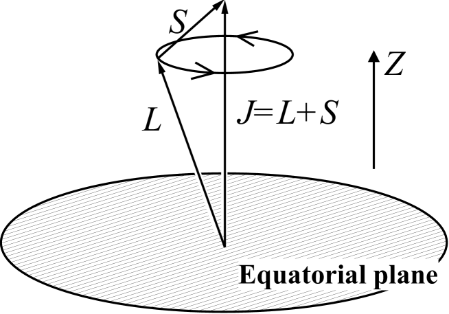
Fig. 3: A schematic picture of the precession of orbit and spin vector, to the leading order in $S$. The vector $J$ represents the total angular momentum of the particle. The vector $L$ is orthogonal to the orbital plane and reduces to the orbital angular momentum in the Newtonian limit. In the relativistic case, however, these vectors should not be regarded as well-defined.

Next we consider the evolution of the spin vector. To the linear order in $S$, the equations to be solved are

$$\dot{\zeta}^{0} = A\zeta^{1}+C\zeta^{2}\tilde{\theta}-Sv^{0}\zeta^{a}R_{a},$$

$$\dot{\zeta}^{1} = A\zeta^{0}+B\zeta^{3}+E\zeta^{2},$$

$$\dot{\zeta}^{2} = \left(C\zeta^{0}+D\zeta^{3}\right)\tilde{\theta}-E\zeta^{1},$$

$$\dot{\zeta}^{3} = -B\zeta^{1}-D\zeta^{2}\tilde{\theta}-Sv^{3}\zeta^{a}R_{a}.$$ (11.58)

The third equation is written down explicitly as

$$\dot{\zeta}^{2}=-\bar{\theta}\zeta_{\parallel}\kappa\sin\phi\cos\phi,$$ (11.59)

where

$$\kappa:=\alpha D-\beta C-\mathchar 28938\relax_{p}\omega_{3}r.$$ (11.60)

Thus we find

$$\zeta^{2}=-\zeta_{\perp}+{\theta_{0}\zeta_{\parallel}\kappa\over 4\mathchar 28938\relax_{p}}\cos 2\phi.$$ (11.61)

Since the spin vector $S^{a}$ is itself of $O(S)$ already, the effect of the second term is always unimportant as long as we neglect corrections of $O(S^{2})$ to the orbit.

The remaining three equations determine $\alpha$, $\beta$ and $\mathchar 28938\relax_{p}$. Corrections of $O(S)$ to $\alpha$ and $\beta$ are less interesting because they remain to be small however long the time passes. On the other hand, the correction to $\mathchar 28938\relax_{p}$ will cause a big effect after a sufficiently long lapse of time because it appears in the combination of $\mathchar 28938\relax_{p}\tau$. The small phase correction will be accumulated to become large. Hence, we solve $\mathchar 28938\relax_{p}$ to the next leading order. Eliminating $\zeta^{0}$ and $\zeta^{3}$ from these three equations, we obtain

$$\left[(B^{2}-A^{2})-\mathchar 28938\relax_{p}^{2}\right]={S_{\perp}\over\xi}\left({AC-BD\over r}-\mathchar 28938\relax_{p}^{2}\omega_{3}\right).$$ (11.62)

Then after a straightforward calculation, we find

$$\mathchar 28938\relax_{p}^{2}={M\over r^{3}}\left\{1-{3S_{\perp}\over r^{3/2}}{\pm\sqrt{M}\left(2r^{2}-3Mr+a^{2}\right)+ar^{1/2}(M-r)\over r^{2}-3Mr\pm 2a\sqrt{Mr}}\right\}.$$ (11.63)

As noted above, $\mathchar 28938\relax_{p}\neq\mathchar 28938\relax_{\varphi}$ for $S_{\perp}\not=0$. The difference $\mathchar 28938\relax_{p}-\mathchar 28938\relax_{\varphi}$ gives the angular velocity of the precession of the spin vector, as depicted in Fig. 3.

11.3 Gravitational waves and energy loss rate

We now proceed to the calculation of the source terms in the Teukolsky equation and evaluate the gravitational wave flux. For this purpose, we must write down the expression of the energy momentum tensor of the spinning particle explicitly. We rewrite the tetrad components of the energy momentum tensor in the following way:

$$T^{ab} = \mu\int d\tau\left\{u^{(a}v^{b)}{\delta^{(4)}(x-z(\tau))\over\sqrt{-g}}-e^{(a}_{~{}\,\nu}e^{b)}_{~{}\rho}\nabla_{\mu}S^{\mu\nu}v^{\rho}{\delta^{(4)}(x-z(\tau))\over\sqrt{-g}}\right\}$$ (11.64)

$$= \mu\int d\tau\Biggl{\{}\left[u^{(a}v^{b)}+\omega_{dc}^{~{}\,(a}v^{b)}S^{dc}-\omega_{dc}^{~{}\,(a}S^{b)d}v^{c}\right]{\delta^{(4)}(x-z(\tau))\over\sqrt{-g}}$$

$$\qquad-{1\over\sqrt{-g}}\partial_{\mu}\left(S^{\mu(a}v^{b)}\delta^{(4)}(x-z(\tau))\right)\Biggr{\}}$$

$$=: \mu\int d\tau\left\{A^{ab}{\delta^{(4)}(x-z(\tau))\over\sqrt{-g}}+{1\over\sqrt{-g}}\partial_{\mu}\left(B^{\mu ab}\delta^{4}(x-z(\tau))\right)\right\}.$$

The last line gives the definition of $A^{ab}$ and $B^{\mu ab}$. Then the source term of the Teukolsky equation is given by Eq. (2.14) with Eqs. (2.15).

As we will see shortly, the terms proportional to $S_{\parallel}$ in the energy momentum tensor do not contribute to the energy or angular momentum fluxes at linear order in $S$. In other words, the energy and angular momentum fluxes are the same for all orbits having the same $S_{\perp}$. Thus, we ignore these terms in the following discussion. Further we recall that the particle can stay in the equatorial plane if $S_{\parallel}=0$. Hence we fix $\theta=\pi/2$ in the following calculations.

Using the formula (2.13), we obtain the amplitude of gravitational waves at infinity as

$$\tilde{Z}^{\infty}_{\ell m\omega}=\tilde{Z}^{nn}_{\ell m\omega}+\tilde{Z}^{\bar{m}n}_{\ell m\omega}+\tilde{Z}^{\bar{m}\bar{m}}_{\ell m\omega},$$ (11.65)

where

$$\tilde{Z}^{nn}_{\ell m\omega} ={i\sqrt{2\pi}\over\omega B^{in}_{\ell m\omega}}\delta\left(\omega-m\mathchar 28938\relax\right)\left({dt\over d\tau}\right)^{-1}\left[A_{nn}-i\omega B^{t}_{nn}+imB^{\varphi}_{nn}-B^{r}_{nn}{\partial\over\partial r}\right]$$

$$\times \left[L^{{\dagger}}_{1}\rho^{-4}\left(L^{{\dagger}}_{2}\rho^{3}{}_{-2}S^{a\omega}_{\ell m}\right)\right]_{\theta=\pi/2}{1\over r\mathchar 28929\relax}R^{in}_{\ell m\omega}\Biggr{|}_{r=r_{0}},$$

$$\tilde{Z}^{\bar{m}n}_{\ell m\omega} = {i\sqrt{\pi}\over\omega B^{in}_{\ell m\omega}}\delta\left(\omega-m\mathchar 28938\relax\right)\left({dt\over d\tau}\right)^{-1}\left[A_{\bar{m}n}-i\omega B^{t}_{\bar{m}n}+imB^{\varphi}_{\bar{m}n}-B^{r}_{\bar{m}n}{\partial\over\partial r}\right]$$

$$\times \left(L^{{\dagger}}_{2}{}_{-2}S^{a\omega}_{\ell m}\right)_{\theta=\pi/2}{1\over\sqrt{\mathchar 28929\relax}}\left[2{\partial\over\partial r}-{2iK\over\mathchar 28929\relax}-{4\over r}\right]R^{in}_{\ell m\omega}\Biggr{|}_{r=r_{0}},$$

$$\tilde{Z}^{\bar{m}\bar{m}}_{\ell m\omega} = {i\sqrt{\pi}\over\omega B^{in}_{\ell m\omega}}\delta\left(\omega-m\mathchar 28938\relax\right)\left({dt\over d\tau}\right)^{-1}\left[A_{\bar{m}\bar{m}}-i\omega B^{t}_{\bar{m}\bar{m}}+imB^{\varphi}_{\bar{m}\bar{m}}-B^{r}_{\bar{m}\bar{m}}{\partial\over\partial r}\right]$$

$$\times \left({}_{-2}S^{a\omega}_{\ell m}\right)_{\theta=\pi/2}\left[{\partial^{2}\over\partial r^{2}}-2\left({1\over r}+{iK\over\mathchar 28929\relax}\right){\partial\over\partial r}-\left({iK\over\mathchar 28929\relax}\right)_{,r}+{2iK\over\mathchar 28929\relax r}-{K^{2}\over\mathchar 28929\relax^{2}}\right]R^{in}_{\ell m\omega}\Biggr{|}_{r=r_{0}},$$

and

$$A_{nn} = {1\over 4}{1\over 1-\xi^{2}}\left\{1-S_{\perp}\left((2\omega_{1}+\omega_{3})\xi+\omega_{2}\right)\right\},$$

$$B^{\mu}_{nn} = {1\over 4r}S_{\perp}{1\over 1-\xi^{2}}\left({r^{2}+a^{2}\over\sqrt{\mathchar 28929\relax}}\xi+a,~{}-\sqrt{\mathchar 28929\relax}\xi,~{}0,~{}{a\over\sqrt{\mathchar 28929\relax}}\xi+1\right),$$

$$A_{\bar{m}n} = {i\over 4\sqrt{2}}{1\over 1-\xi^{2}}\left\{2\xi-S_{\perp}\left(\omega_{1}\xi^{2}-4\omega_{2}\xi-\omega_{3}\right)\right\},$$

$$B^{\mu}_{\bar{m}n} = {i\over 4\sqrt{2}r}S_{\perp}{1\over 1-\xi^{2}}\left({r^{2}+a^{2}\over\sqrt{\mathchar 28929\relax}}\xi^{2}+a\xi,~{}-\sqrt{\mathchar 28929\relax}(1+\xi^{2}),~{}0,~{}{a\over\sqrt{\mathchar 28929\relax}}\xi^{2}+\xi\right),$$

$$A_{\bar{m}\bar{m}} = -{1\over 2}{1\over 1-\xi^{2}}\left\{\xi^{2}+S_{\perp}\left(\omega_{2}(1+2\xi^{2})+\omega_{3}\xi\right)\right\},$$

$$B^{\mu}_{\bar{m}\bar{m}} = {1\over 2r}S_{\perp}{1\over 1-\xi^{2}}\left(0,~{}\sqrt{\mathchar 28929\relax}\xi,~{}0,~{}0\right).$$ (11.67)

The Lorentz factor $dt/d\tau$ which appears in Eqs. (LABEL:sp:Ztilde) is calculated from Eqs. (11.53) as

$${dt\over d\tau}={1\ \over r\sqrt{1-\xi^{2}}}\left(a\xi+{r^{2}+a^{2}\over\sqrt{\mathchar 28929\relax}}\right).$$ (11.68)

In general, as we have seen in the preceding sections, when the orbit is quasi-periodic the Fourier components of gravitational waves will have a discrete spectrum;

$$\tilde{Z}_{\ell m\omega}=\sum_{n}\delta(\omega-\omega_{n})Z_{\ell m\omega_{n}}\,.$$ (11.69)

Then the time-averaged energy flux and the $z$-component of the angular momentum flux are given by the formulas (2.31) and (2.32), respectively. In the present case, since we may regard the orbits to be on the equatorial plane, the index $n$ degenerates to the angular index $m$ and $\omega_{n}$ is simply given by $m\mathchar 28938\relax_{\varphi}$ $(n=m)$. Hence we eliminate the index $n$ in the following discussion. Here we mention the effect of nonzero $S_{\parallel}$. If we recall that all the terms which are proportional to $S_{\parallel}$ have the time dependence of $e^{\pm i\mathchar 28938\relax_{p}\tau}$, we find that they give the contribution to the side bands. That is to say, their contributions in $\tilde{Z}_{\ell m\omega}$ are all proportional to $\delta(\omega-m\mathchar 28938\relax\pm\mathchar 28938\relax_{p})$. Then, since the energy and angular momentum fluxes are quadratic in $Z_{\ell m\omega_{n}}$, they are not affected by the presence of $S_{\parallel}$ as long as we are working only up to linear order in $S$.

As before, in order to express the post-Newtonian corrections to the energy flux, we define $\eta_{\ell m\omega}$ as

$$\left({dE\over dt}\right)_{\ell m}={1\over 2}\left({dE\over dt}\right)_{\rm N}\eta_{\ell m},$$ (11.70)

where $(dE/dt)_{\rm N}$ is the Newtonian quadrupole formula defined by Eq. (4.42).

We calculate $\eta_{\ell m}$ up to 2.5PN order. Keeping the $S$-dependent terms, the results are

$$\eta^{(s)}_{2\pm 2} = \left(-{19\over 3}v^{3}9qv^{4}+{2134\over 63}v^{5}\right)\hat{s},$$

$$\eta^{(s)}_{2\pm 1} = \left(-{1\over 12}v^{3}-{1\over 8}qv^{4}-{535\over 1008}v^{5}\right)\hat{s},$$

$$\eta^{(s)}_{3\pm 3} = -{10935\over 896}v^{5}\hat{s},$$

$$\eta^{(s)}_{3\pm 2} = {20\over 63}v^{5}\hat{s},$$

$$\eta^{(s)}_{3\pm 1} = -{1\over 8064}v^{5}\hat{s},$$ (11.71)

where $q=a/M$ and $\hat{s}:=S_{\perp}/M$. The rest of $\eta^{(s)}_{\ell m}$ are all of higher order. We should mention that if we regard the spinning particle as a model of a black hole or neutron star, $S$ is of order $\mu$. Therefore the correction due to $S$ is small compared with the $S$-independent terms in the test particle limit $\mu/M\ll 1$.

Putting all together, we obtain

$$\left\langle dE\over dt\right\rangle=\left(dE\over dt\right)_{N}\Biggl{[} 1-{1247\over 336}v^{2}+\left(4\pi-{73\over 12}q-{25\over 4}\hat{s}\right)v^{3}$$ (11.72)

$$+\left(-{44711\over 9072}+{33\over 16}q^{2}+{71\over 8}q\hat{s}\right)v^{4}$$

$$+\left(-{8191\over 672}\pi+{3749\over 336}q+{2403\over 112}\hat{s}\right)v^{5}\Biggr{]}.$$

Since $v$ is defined in terms of the coordinate radius of the orbit, the expansion with respect to $v$ does not have a clear gauge-invariant meaning. In particular, for the purpose of the comparison with the standard post-Newtonian calculations it is better to write the result by means of the angular velocity observed at infinity. Using the post-Newtonian expansion of Eq. (11.54)

$$M\mathchar 28938\relax_{\varphi}=v^{3}\left(1-\left({3\over 2}\hat{s}+q\right)v^{3}+{3\over 2}q\hat{s}v^{4}+O\left(v^{6}\right)\right),$$ (11.73)

Eq. (11.72) can be rewritten as

$$\left\langle dE\over dt\right\rangle=\widetilde{\left({dE\over dt}\right)}_{\rm N}\Biggl{[} 1-{1247\over 336}x^{2}+\left(4\pi-{11\over 4}q-{5\over 4}\hat{s}\right)x^{3}$$ (11.74)

$$+\left(-{44711\over 9072}+{33\over 16}q^{2}+{31\over 8}q\hat{s}\right)x^{4}$$

$$+\left(-{8191\over 672}\pi+{59\over 16}q-{13\over 16}\hat{s}\right)x^{5}\Biggr{]},$$

where $x=(M\mathchar 28938\relax_{\varphi})^{1/3}$ and $\widetilde{(dE/dt)}_{\rm N}$ is the Newtonian quadrupole formula expressed in terms of $x$, Eq. (6.6). Since there is no sideband contribution in the present case, the angular momentum flux is simply given by $\langle dJ_{z}/dt\rangle=\mathchar 28938\relax_{\varphi}^{-1}\langle dE/dt\rangle_{\rm GW}$. The result (11.74) is consistent with the one obtained by the standard post-Newtonian approach[41, 54] to the 2PN order in the limit $\mu/M\to 0$. The $\hat{s}$-dependent term of order $x^{5}$ is the one which is newly obtained by the black hole perturbation approach[18].

12 Black hole absorption

When a particle moves around a Kerr black hole, it radiates gravitational waves. Some of those waves are absorbed by the black hole. We calculate such absorption of gravitational waves induced by a particle of mass $\mu$ in circular orbit on the equatorial plane around a Kerr black hole of Mass $M$.

The post-Newtonian approximation of the absorption of gravitational waves into the black hole horizon was first calculated by Poisson and Sasaki in the case when a test particle is in a circular orbit around a Schwarzschild black hole[21]. In this case, the effect of the black hole absorption is found to appear at $O(v^{8})$ compared to the flux emitted to infinity and it turns out to be negligible for the orbital evolution of coalescing compact binaries in the near future laser interferometer’s band. On the other hand, the black hole absorption appears at $O(v^{5})$ if a black hole is rotating. That calculation was done by Tagoshi, Mano, and Takasugi[24].

In order to calculate the post-Newtonian expansion of ingoing gravitational waves into a Schwarzschild black hole, Poisson and Sasaki[21] used two type of representations of a solution of the homogeneous Teukolsky equation. One is expressed in terms of the spherical Bessel functions which can be used at large radius, and the other is expressed in terms of a hypergeometric function which can be used near the horizon. Then two type of expressions are matched at some region where both formulas can be applied. They got formulas for a solution of the Teukolsky equation which can be used to calculate ingoing gravitational waves to $O(v^{13})$, although they gave formulas for ingoing waves only to $O(v^{8})$.

Here, we first review the method found by Mano, Suzuki and Takasugi[23], since it is the only existing method by which higher order post-Newtonian terms of the gravitational waves absorbed into a rotating black hole can be calculated. We note that this method is also the only existing method that can be used to calculate the gravitational waves emitted to infinity to an arbitrarily high post-Newtonian order. Then we calculate the energy flux absorbed into the horizon to $O(v^{13})$, i.e., $O(v^{8})$ beyond the lowest order flux absorbed into the horizon, for circular orbits on the equatorial plane of a Kerr black hole.

12.1 Analytic solutions of the homogeneous Teukolsky equation

Analytic series solutions of the homogeneous Teukolsky equation were found by Mano, Suzuki and Takasugi[23] and various properties of the solution were discussed by Mano and Takasugi[55]. Here, we follow the notation of Ref. ? except that we focus on the case of spin weight $s=-2$. In this method, the solution of the radial Teukolsky equation (2.3) is represented by two kinds of expansion. One is given by a series of hypergeometric functions and the other by a series of Coulomb wave functions. The former is convergent at horizon and the latter at infinity. Then the matching of these two solutions are done exactly in the overlapping region of convergence.

First we consider the solution expressed in terms of hypergeometric functions. The solution which satisfies the ingoing wave boundary condition at horizon is expressed as

$$R^{{\rm in}\,\nu}= e^{i\epsilon\kappa x}(-x)^{2-i\epsilon_{+}}(1-x)^{i\epsilon_{-}}$$ (12.1)

$$\times\sum_{n=-\infty}^{\infty}a_{n}^{\nu}F(n+\nu+1-i\tau,-n-\nu-i\tau,3-2i\epsilon_{+};x),$$

where $F(a,b,c,x)$ is the hypergeometric function and

$$x=-{\omega(r-r_{+})\over\epsilon\kappa}\,,\quad\kappa=\sqrt{1-q^{2}}\,,\quad\tau={{\epsilon-mq}\over\kappa}\,,\quad\epsilon_{\pm}={\epsilon\pm\tau\over 2}\,.$$ (12.2)

The coefficients $a_{n}^{\nu}$ obey a three terms recurrence relation,

$$\alpha_{n}^{\nu}a_{n+1}^{\nu}+\beta^{\nu}_{n}a_{n}^{\nu}+\gamma^{\nu}_{n}a_{n-1}^{\nu}=0,$$ (12.3)

where

$$\alpha_{n}^{\nu} = {i\epsilon\kappa(n+\nu-1+i\epsilon)(n+\nu-1-i\epsilon)(n+\nu+1+i\tau)\over{(n+\nu+1)(2n+2\nu+3)}}\,,$$ (12.4)

$$\beta_{n}^{\nu} = -\lambda-2+(n+\nu)(n+\nu+1)+\epsilon^{2}+\epsilon(\epsilon-mq)$$ (12.6)

$$\hskip 8.53581pt+{\epsilon(\epsilon-mq)(4+\epsilon^{2})\over{(n+\nu)(n+\nu+1)}}\,,$$

$$\gamma_{n}^{\nu} = -{i\epsilon\kappa(n+\nu+2+i\epsilon)(n+\nu+2-i\epsilon)(n+\nu-i\tau)\over{(n+\nu)(2n+2\nu-1)}}\,.$$ (12.7)

The series converges if $\nu$ satisfies the equation,

$$R_{n}(\nu)L_{n-1}(\nu)=1,$$ (12.8)

where $R_{n}(\nu)$ and $L_{n}(\nu)$ are the continued fractions defined by

$$R_{n}(\nu) \equiv {a_{n}^{\nu}\over a_{n-1}^{\nu}}=-{\gamma_{n}^{\nu}\over\beta_{n}^{\nu}+\alpha_{n}^{\nu}R_{n+1}(\nu)}\,,$$ (12.9)

$$L_{n}(\nu) \equiv {a_{n}^{\nu}\over a_{n+1}^{\nu}}=-{\alpha_{n}^{\nu}\over\beta_{n}^{\nu}+\gamma_{n}^{\nu}L_{n-1}(\nu)}\,.$$ (12.10)

The range of convergence is $0\leq(-x)<\infty$ for physical $x$. We can prove that if $\nu$ is a solution to Eq. (12.8), then so is $-\nu-1$. Since we can set $n$ in Eq. (12.8) to an arbitrary integer, a convenient choice is to put $n=1$. Further, for convenience, we may set $a_{0}^{\nu}=a_{0}^{-\nu-1}=1$. It then follows that we have

$$a_{-n}^{-\nu-1}=a_{n}^{\nu}\,.$$ (12.11)

This implies $R^{{\rm in}\,\nu}=R^{{\rm in}\,-\nu-1}\equiv R^{\rm in}$. Consequently, for $(-x)>0$, Eq. (12.1) can be rewritten as

$$R^{\rm in}=e^{i\epsilon\kappa}(R_{0}^{\nu}+R_{0}^{-\nu-1}),$$ (12.12)

where

$${R}_{0}^{\nu} = e^{-i\epsilon\kappa\tilde{x}}(\tilde{x})^{\nu+i\epsilon_{+}}(\tilde{x}-1)^{-s-i\epsilon_{+}}$$ (12.15)

$$\times\sum_{n=-\infty}^{\infty}\frac{\mathchar 28928\relax(3-2i\epsilon_{+})\mathchar 28928\relax(2n+2\nu+1)}{\mathchar 28928\relax(n+\nu+1-i\tau)\mathchar 28928\relax(n+\nu+3-i\epsilon)}a_{n}^{\nu}$$

$$\times\tilde{x}^{n}F(-n-\nu-i\tau,-n-\nu+2-i\epsilon,-2n-2\nu;\frac{1}{\tilde{x}}),$$

where

$$\tilde{x}=1-x={\omega(r-r_{-})\over{\epsilon\kappa}}\,.$$ (12.16)

Since $\nu-(-\nu-1)=2\nu+1$ is not an integer in general, the solutions $R_{0}^{\nu}$ and $R_{0}^{-\nu-1}$ form a pair of independent solutions.

The other series solution which is convergent at infinity is expressed in terms of the Coulomb wave functions; [56]

$${R}_{C}^{\nu}=\tilde{z}\left(1-{\epsilon\kappa\over{\tilde{z}}}\right)^{2-i\epsilon_{+}}\sum_{n=-\infty}^{\infty}(-i)^{n}\frac{(\nu-1-i\epsilon)_{n}}{(\nu+3+i\epsilon)_{n}}a_{n}^{\nu}F_{n+\nu}(\tilde{z}),$$ (12.17)

where $\tilde{z}=\omega(r-r_{-})=\epsilon\kappa\tilde{x}$, $(a)_{n}=\mathchar 28928\relax(n+a)/\mathchar 28928\relax(a)$, and $F_{n+\nu}(z)$ is the Coulomb wave function given by

$$F_{n+\nu}(z) = e^{-iz}(2z)^{n+\nu}z{\mathchar 28928\relax(n+\nu+3+i\epsilon)\over{\mathchar 28928\relax(2n+2\nu+2)}}$$

$$\times{\rm\mathchar 28936\relax}(n+\nu+3+i\epsilon,2n+2\nu+2;2iz),$$

where ${\rm\mathchar 28936\relax}(a,b,z)$ is the regular confluent hypergeometric function[57]. A crucial observation made by Mano, Suzuki and Takasugi[23] is that the coefficients ${a_{n}^{\nu}}$ obey the same recurrence relation as that for the hypergeometric type solution, Eq. (12.3). The series (12.17) converges in the range $\tilde{z}>\epsilon\kappa$ if $\nu$ is a solution of Eq. (12.8). The solution $R_{C}^{\nu}$ can be decomposed into a pair of solutions, a purely incoming wave at infinity $R_{+}^{\nu}$ and a purely outgoing wave at infinity $R_{-}^{\nu}$. Explicitly, we have

$$R_{C}^{\nu}=R_{+}^{\nu}+R_{-}^{\nu},$$ (12.18)

where

$$R_{+}^{\nu} =2^{\nu}e^{-\pi\epsilon}e^{i\pi(\nu+3)}\frac{\mathchar 28928\relax(\nu+3+i\epsilon)}{\mathchar 28928\relax(\nu-1-i\epsilon)}e^{-i\tilde{z}}\tilde{z}^{\nu+i\epsilon_{+}}(\tilde{z}-\epsilon\kappa)^{2-i\epsilon_{+}}$$ (12.20)

$$\times\sum_{n=-\infty}^{\infty}i^{n}a_{n}^{\nu}(2\tilde{z})^{n}{\rm\mathchar 28937\relax}(n+\nu+3+i\epsilon,2n+2\nu+2;2i\tilde{z}),$$

$$R_{-}^{\nu} =2^{\nu}e^{-\pi\epsilon}e^{-i\pi(\nu-1)}e^{i\tilde{z}}\tilde{z}^{\nu+i\epsilon_{+}}(\tilde{z}-\epsilon\kappa)^{2-i\epsilon_{+}}\sum_{n=-\infty}^{\infty}i^{n}$$ (12.22)

$$\times\frac{(\nu-1-i\epsilon)_{n}}{(\nu+3+i\epsilon)_{n}}a_{n}^{\nu}(2\tilde{z})^{n}{\rm\mathchar 28937\relax}(n+\nu-1-i\epsilon,2n+2\nu+2;-2i\tilde{z}),$$

where ${\rm\mathchar 28937\relax}(a,b,z)$ is the irregular confluent hypergeometric function[57]. By definition, the upgoing solution $R^{\rm up}$ is given by

$$R^{\rm up}=R_{-}^{\nu}\,.$$ (12.23)

We see that the above two kinds of solutions are convergent in the common region $1<\tilde{x}<\infty$. Then comparing the asymptotic behaviors of $R^{\nu}_{0}$ and $R^{\nu}_{C}$ for $\tilde{x}\to\infty$, we find that they have the same characteristic exponent, $\sim\tilde{x}^{\nu}$, hence describe the same solution up to the normalization factor. Therefore by comparing each power of $\tilde{x}$ we have

$$R_{0}^{\nu}=K_{\nu}R^{\nu}_{C},$$ (12.24)

where

$${K}_{\nu} = \frac{(2\epsilon\kappa)^{-\nu-2-{\tilde{r}}}2^{2}i^{\tilde{r}}\mathchar 28928\relax(3-2i\epsilon_{+})\mathchar 28928\relax({\tilde{r}}+2\nu+1)\mathchar 28928\relax({\tilde{r}}+2\nu+2)}{\mathchar 28928\relax(\nu+1-i\tau)\mathchar 28928\relax(\nu+3-i\epsilon)\mathchar 28928\relax({\tilde{r}}+\nu+3+i\epsilon)}$$ (12.28)

$$\times\frac{\mathchar 28928\relax(\nu+1+i\tau)\mathchar 28928\relax(\nu-1+i\epsilon)}{\mathchar 28928\relax({\tilde{r}}+\nu+1+i\tau)\mathchar 28928\relax({\tilde{r}}+\nu-1+i\epsilon)}$$

$$\times\overline{\left(\sum_{n={\tilde{r}}}^{\infty}\frac{({\tilde{r}}+2\nu+1)_{n}}{(n-{\tilde{r}})!}\frac{(\nu-1-i\epsilon)_{n}}{(\nu+3+i\epsilon)_{n}}a_{n}^{\nu}\right)}$$

$$\times\left(\sum_{n=-\infty}^{{\tilde{r}}}\frac{(-1)^{n}}{({\tilde{r}}-n)!({\tilde{r}}+2\nu+2)_{n}}\frac{(\nu-1-i\epsilon)_{n}}{(\nu+3+i\epsilon)_{n}}a_{n}^{\nu}\right)^{-1},$$

where $\tilde{r}$ can be any integer and ${K}_{\nu}$ is independent of the choice of ${\tilde{r}}$.

The gravitational wave absorbed into the black hole is expressed by Eq. (2.12). Hence we need to know the amplitudes $B^{\rm inc}$ and $B^{\rm trans}$ of $R^{\rm in}$ and $C^{\rm trans}$ of $R^{\rm up}$, defined in Eq. (2.7). The asymptotic ingoing amplitude at horizon, $B^{\rm trans}$, of $R^{\rm in}$ is readily obtained from Eq. (12.1) as

$$B^{\rm trans}=\left(\frac{\epsilon\kappa}{\omega}\right)^{2s}e^{i\epsilon_{+}\ln\kappa}\sum_{n=-\infty}^{\infty}a_{n}^{\nu}\,.$$ (12.29)

Similarly, the asymptotic outgoing amplitude at infinity, $C^{\rm trans}$, of $R^{\rm up}$ is obtained from Eq. (12.22) as

$$C^{\rm trans}= 2^{1+i\epsilon}e^{-\pi\epsilon/2}e^{-{\pi\over 2}i(\nu-1)}\omega^{3}e^{i\epsilon\ln\epsilon}$$ (12.30)

$$\quad\times\left[\sum_{n=-\infty}^{\infty}{(\nu-1-i\epsilon)_{n}\over(\nu+3+i\epsilon)_{n}}(-1)^{n}a_{n}^{\nu}\right].$$

On the other hand, a bit of work is necessary to obtain the asymptotic incoming amplitude at infinity, $B^{\rm inc}$, of $R^{\rm in}$. Setting the asymptotic behavior of $R_{C}^{\nu}$ at $z\to\infty$ as

$$R_{C}^{\nu}\to A_{+}^{\nu}z^{-1}e^{-i(z+\epsilon\ln z)}+A_{-}^{\nu}z^{3}e^{i(z+\epsilon\ln z)},$$ (12.31)

we find

$$A_{+}^{\nu}=2^{-3-i\epsilon}e^{i(\pi/2)(\nu+3)}e^{-\pi\epsilon/2}\frac{\mathchar 28928\relax(\nu+3+i\epsilon)}{\mathchar 28928\relax(\nu-1-i\epsilon)}\sum_{n=-\infty}^{\infty}a_{n}^{\nu},$$

$$A_{-}^{\nu}=2^{1+i\epsilon}e^{-i(\pi/2)(\nu-1)}e^{-\pi\epsilon/2}\sum_{n=-\infty}^{\infty}(-1)^{n}\frac{(\nu-1-i\epsilon)_{n}}{(\nu+3+i\epsilon)_{n}}a_{n}^{\nu}.$$ (12.32)

Because of Eq. (12.11), $A_{\pm}^{\nu}$ and $A_{\pm}^{-\nu-1}$ are related to each other as

$$A_{+}^{-\nu-1}=-ie^{-i\pi\nu}{\sin\pi(\nu+i\epsilon)\over\sin\pi(\nu-i\epsilon)}A_{+}^{\nu}\,,$$

$$A_{-}^{-\nu-1}=ie^{i\pi\nu}A_{-}^{\nu}\,.$$ (12.33)

With the help of the above relations, we find from Eqs. (12.12) and (12.24) the asymptotic amplitudes of $R^{\rm in}$ at infinity as

$$B^{\rm inc} = \frac{e^{i\epsilon\kappa}}{\omega}\left[{K}_{\nu}-ie^{-i\pi\nu}\frac{\sin\pi(\nu+i\epsilon)}{\sin\pi(\nu-i\epsilon)}{K}_{-\nu-1}\right]A_{+}^{\nu}e^{-i\epsilon\ln\epsilon},$$

$$B^{\rm ref} = e^{i\epsilon\kappa}\omega^{3}\left[{K}_{\nu}+ie^{i\pi\nu}{K}_{-\nu-1}\right]A_{-}^{\nu}e^{i\epsilon\ln\epsilon}.$$ (12.34)

So far our discussion has been on exact analytic series expressions for the homogeneous Teukolsky functions. Now we consider their post-Minkowski expansion by assuming $\epsilon\ll 1$. Provided we set $a_{0}^{\nu}=1$, we see from Eqs. (12.7) that $\alpha_{n}^{\nu}$, $\gamma_{n}^{\nu}=O(\epsilon)$ and $\beta_{n}^{\nu}=O(1)$ unless the value of $\nu$ is such that the denominator in the expression of $\alpha_{n}^{\nu}$ or $\gamma_{n}^{\nu}$ happens to vanish or $\beta_{n}^{\nu}$ happens to vanish in the limit $\epsilon\to 0$. Except for such an exceptional case, it is easy to see from Eq. (12.3) that the order of $a_{n}^{\nu}$ in $\epsilon$ increases as $|n|$ increases. Thus the series solution naturally gives the post-Minkowski expansion.

For the moment, let us assume that the above mentioned exceptional case does not happen for $n=0$. Then we have $R_{1}(\nu)=O(\epsilon)$ and $L_{0}(\nu)=O(1/\epsilon)$. This implies $\beta_{0}^{\nu}+\gamma_{0}^{\nu}L_{-1}(\nu)=O(\epsilon^{2})$. Then assuming $L_{-1}(\nu)=O(\epsilon)$, we must have $\beta_{0}^{\nu}=O(\epsilon^{2})$. Using the expansion of $\lambda$ given by Eq. (3.1), we then find $\nu=\ell+O(\epsilon^{2})$ or $\nu=-\ell-1+O(\epsilon^{2})$. Since we know that $-\nu-1$ is a solution if $\nu$ is so, we may take the solution $\nu=\ell+O(\epsilon^{2})$ without loss of generality. Then the assumptions that $R_{1}(\nu)=1/L_{0}(\nu)=O(\epsilon)$ and $L_{-1}(\nu)=O(\epsilon)$ are justified. Further it is easily seen that $R_{n}(\nu)=O(\epsilon)$ for all $n>0$. On the other hand, for $n<0$, $\alpha_{n}^{\nu}=O(1)$ at $n=-\ell-1$ and $\beta_{n}^{\nu}=O(\epsilon^{2})$ at $n=-2\ell-1$. Thus we have $L_{-\ell-1}(\nu)=O(1)$ and $L_{-2\ell-1}(\nu)=O(1/\epsilon)$. To summarize, we have

$$R_{n}(\nu)={a_{n}^{\nu}\over a_{n-1}^{\nu}}=O(\epsilon)\quad\hbox{\rm for all}~{}n>0,$$

$$L_{-\ell-1}(\nu)={a_{-\ell-1}^{\nu}\over a_{-\ell}^{\nu}}=O(1),\quad L_{-2\ell-1}(\nu)={a_{-2\ell-1}^{\nu}\over a_{-2\ell}^{\nu}}=O(1/\epsilon),$$

$$L_{n}(\nu)={a_{n}^{\nu}\over a_{n+1}^{\nu}}=O(\epsilon)\quad\hbox{\rm for all the other}~{}n<0.$$ (12.35)

With the above results, the post-Minkowski expansion of the homogeneous Teukolsky functions can be obtained with arbitrary accuracy by solving Eq. (12.8) to a desired order and by summing up the terms to a sufficiently large $|n|$. For our present purpose, we need $\nu$ which is accurate to $O(\epsilon^{2})$. Solving Eq. (12.8) to this order, we find

$$\nu = \ell+{\epsilon^{2}\over 2\ell+1}\Biggl{[}-2-{4\over\ell(\ell+1)}$$ (12.36)

$$\qquad+{(\ell-1)^{2}(\ell+3)^{2}\over(2\ell+1)(2\ell+2)(2\ell+3)}-{(\ell-2)^{2}(\ell+2)^{2}\over(2\ell-1)2\ell(2\ell+1)}\Biggr{]}.$$

Interestingly, $\nu$ is found to be independent of the azimuthal eigenvalue $m$ to $O(\epsilon^{2})$.

The post-Newtonian expansion in the near zone is given by further assuming $\epsilon\ll z\ll 1$ in the series solution (12.17) and expand it in powers $z$. For evaluation of the black hole absorption, we need the post-Newtonian expansion of $R^{\rm up}$ which is obtained from Eq. (12.22). The explicit post-Newtonian formula for $R^{\rm up}$ and the asymptotic amplitudes $B^{\rm inc}$, $B^{\rm trans}$ and $C^{\rm trans}$ to $O(\epsilon^{2})$ are given in Appendix H.

12.2 Absorption rate to $O(v^{8})$

In this subsection, we evaluate the energy absorption rate by a black hole. The energy flux formula is given by Teukolsky and Press[58] as

$$\left(dE_{\rm hole}\over dtd\mathchar 28938\relax\right)=\sum_{\ell m}\int d\omega{{{}_{2}S_{\ell m}^{2}}\over 2\pi}{{128\omega k(k^{2}+4{\tilde{\epsilon}}^{2})(k^{2}+16{\tilde{\epsilon}}^{2})(2Mr_{+})^{5}}\over|C|^{2}}|\tilde{Z}^{\rm H}_{\ell m\omega}|^{2},$$ (12.37)

where ${\tilde{\epsilon}}=\kappa/(4r_{+})$ and

$$|C|^{2} = \left((\lambda+2)^{2}+4a\omega m-4a^{2}\omega^{2}\right)\left[\lambda^{2}+36a\omega m-36a^{2}\omega^{2}\right]$$ (12.38)

$$+(2\lambda+3)(96a^{2}\omega^{2}-48a\omega m)+144\omega^{2}(M^{2}-a^{2}).$$

The calculation of $\tilde{Z}^{\rm H}_{\ell m\omega}$ is parallel to the calculation of $\tilde{Z}^{\infty}_{\ell m\omega}$ except that $R^{\rm in}$ is replaced by $R^{\rm up}$. The solution of the geodesic equations are given in section 6. Using that solution, we have the amplitude of the Teukolsky function at the horizon in Eq. (2.12) as

$$\tilde{Z}^{\rm H}_{\ell m\omega} = {{2\pi B^{\rm trans}\delta(\omega-m\mathchar 28938\relax)}\over{2i\omega B^{\rm inc}C^{\rm trans}}}\Bigl{[}R^{{\rm up}}_{\ell m\omega}\{A_{n\,n\,0}+A_{{\bar{m}}\,n\,0}+A_{{\bar{m}}\,{\bar{m}}\,0}\}$$ (12.39)

$$-{dR^{{\rm up}}_{\ell m\omega}\over dr}\{A_{{\bar{m}}\,n\,1}+A_{{\bar{m}}\,{\bar{m}}\,1}\}+{d^{2}R^{{\rm up}}_{\ell m\omega}\over dr^{2}}A_{{\bar{m}}\,{\bar{m}}\,2}\Bigr{]}_{r=r_{0},\theta=\pi/2},$$

$$\equiv \delta(\omega-m\mathchar 28938\relax)Z^{\rm H}_{\ell m}\,.$$

From Eq. (12.37) and (12.39), the time averaged energy absorption rate becomes

$$\left\langle{dE\over dt}\right\rangle_{\rm H} = \sum_{\ell m}\left[{{128\omega k(k^{2}+4{\tilde{\epsilon}}^{2})(k^{2}+16{\tilde{\epsilon}}^{2})(2Mr_{+})^{5}}\over|C|^{2}}|Z^{\rm H}_{\ell m}|^{2}\right]_{\omega=m\mathchar 28938\relax}$$ (12.40)

$$\equiv \sum_{\ell m}\left(dE\over dt\right)_{\ell,m}.$$ (12.41)

As in the case of the Teukolsky function at infinity, we can show that $\bar{Z}^{\rm H}_{\ell,-m,-\omega}$ $=(-1)^{\ell}Z^{\rm H}_{\ell,m,\omega}$. Then, from Eq. (12.41), we have $(dE/dt)_{\ell,-m}=(dE/dt)_{\ell,m}$.

In order to express the post-Newtonian corrections to the black hole absorption, we define $\eta_{\ell,m}^{\rm H}$ as

$$\left({dE\over dt}\right)_{\ell,m}\equiv{1\over 2}\left({dE\over dt}\right)_{N}v^{5}\eta_{\ell,m}^{\rm H}\,,$$ (12.42)

where $(dE/dt)_{N}$ is the Newtonian quadrupole luminosity at infinity, Eq. (4.42). In Appendix I, we show $\eta_{\ell m}$.

The total absorption rate to $O(v^{8})$ beyond the lowest order is given by

$$\left\langle{dE\over dt}\right\rangle_{\rm H} =\left(dE\over dt\right)_{N}\,v^{5}\,\Biggl{[}-{3\over 4}\,{q}^{3}-{1\over 4}\,q+\left(-q-{\frac{33}{16}}\,{q}^{3}\right){v}^{2}$$ (12.43)

$$+\left({7\over 2}\,{q}^{4}+2\,q{B_{2}}+{1\over 2}+6\,{q}^{3}{B_{2}}+{\frac{85}{12}}\,{q}^{2}+3\,{q}^{4}\kappa+{1\over 2}\,\kappa+{13\over 2}\,\kappa\,{q}^{2}\right){v}^{3}$$

$$+\left(-{\frac{4651}{336}}\,{q}^{3}-{\frac{43}{7}}\,q-{\frac{17}{56}}\,{q}^{5}\right){v}^{4}$$

$$+\Bigl{(}{\frac{569}{24}}\,{q}^{2}+{\frac{371}{48}}\,{q}^{4}+18\,{q}^{3}{B_{2}}-{3\over 4}\,{q}^{3}{B_{1}}+2\,\kappa+2+{\frac{33}{4}}\,{q}^{4}\kappa$$

$$+6\,q{B_{2}}+{\frac{163}{8}}\,\kappa\,{q}^{2}+q{B_{1}}\Bigr{)}{v}^{5}$$

$$+\Bigl{(}-{\frac{2718629}{44100}}\,q-4\,{B_{2}}+{\frac{428}{105}}\,\gamma\,q+{2\over 3}\,{\pi}^{2}q+{\frac{428}{105}}\,q\ln 2-4\,q{C_{2}}$$

$$-12\,{q}^{3}{C_{2}}-36\,{q}^{4}{B_{2}}-56\,{q}^{2}{B_{2}}+{\frac{428}{35}}\,{q}^{3}\gamma+{\frac{428}{35}}\,{q}^{3}\ln 2+2\,{q}^{3}{\pi}^{2}$$

$$+{\frac{428}{105}}\,q\ln\kappa+{\frac{428}{105}}\,q{A_{2}}+{\frac{428}{35}}\,{q}^{3}\ln\kappa+6\,{\frac{{q}^{7}}{\kappa}}+{\frac{428}{35}}\,{q}^{3}{A_{2}}-8\,q{{B_{2}}}^{2}$$

$$-24\,{q}^{3}{{B_{2}}}^{2}+{\frac{856}{105}}\,q\ln v+{\frac{856}{35}}\,{q}^{3}\ln v-4\,{\frac{{B_{2}}}{\kappa}}-32\,{\frac{{q}^{3}}{\kappa}}-31\,{\frac{q}{\kappa}}$$

$$+57\,{\frac{{q}^{5}}{\kappa}}+{q}^{5}\kappa+{q}^{4}{B_{1}}-{2\over 3}\,\kappa\,q-{7\over 6}\,\kappa\,{q}^{3}-{4\over 3}\,{q}^{2}{B_{1}}$$

$$-48\,{\frac{{q}^{2}{B_{2}}}{\kappa}}+28\,{\frac{{q}^{4}{B_{2}}}{\kappa}}-24\,{\frac{{q}^{3}{C_{2}}}{\kappa}}-8\,{\frac{q{C_{2}}}{\kappa}}+24\,{\frac{{q}^{6}{B_{2}}}{\kappa}}$$

$$-{\frac{2400247}{19600}}\,{q}^{3}+{\frac{299}{16}}\,{q}^{5}\Bigr{)}{v}^{6}$$

$$+\Bigl{(}{\frac{225}{28}}\,{q}^{5}{B_{3}}-{\frac{41}{28}}\,\kappa\,{q}^{6}+{\frac{86}{7}}+{\frac{8741}{56}}\,{q}^{2}+{\frac{3485}{42}}\,{q}^{4}+{\frac{167}{112}}\,{q}^{6}$$

$$+{\frac{86}{7}}\,\kappa+{\frac{45}{56}}\,q{B_{3}}-{\frac{9}{28}}\,{q}^{5}{B_{1}}+{\frac{899}{168}}\,q{B_{1}}-{\frac{803}{224}}\,{q}^{3}{B_{1}}+{\frac{1665}{224}}\,{q}^{3}{B_{3}}$$

$$+{\frac{2372}{21}}\,{q}^{3}{B_{2}}-{\frac{16}{7}}\,{q}^{5}{B_{2}}+{\frac{719}{12}}\,{q}^{4}\kappa+{\frac{22201}{168}}\,\kappa\,{q}^{2}+{\frac{796}{21}}\,q{B_{2}}\Bigr{)}{v}^{7}$$

$$+\Bigl{(}-{\frac{20542807}{88200}}\,q-12\,{B_{2}}-2\,{B_{1}}+{\frac{1061}{35}}\,\gamma\,q+{\frac{13}{6}}\,{\pi}^{2}q+{\frac{995}{21}}\,q\ln 2$$

$$-12\,q{C_{2}}-36\,{q}^{3}{C_{2}}-{\frac{308}{3}}\,{q}^{4}{B_{2}}-{\frac{1496}{9}}\,{q}^{2}{B_{2}}+{\frac{12197}{140}}\,{q}^{3}\gamma+{\frac{3873}{28}}\,{q}^{3}\ln 2$$

$$+{\frac{47}{8}}\,{q}^{3}{\pi}^{2}+{\frac{1391}{105}}\,q\ln\kappa+{\frac{428}{35}}\,q{A_{2}}+{\frac{5029}{140}}\,{q}^{3}\ln\kappa+{\frac{37}{6}}\,{\frac{{q}^{7}}{\kappa}}+{\frac{1284}{35}}\,{q}^{3}{A_{2}}$$

$$-24\,q{{B_{2}}}^{2}-72\,{q}^{3}{{B_{2}}}^{2}+{\frac{4574}{105}}\,q\ln v+{\frac{8613}{70}}\,{q}^{3}\ln v-12\,{\frac{{B_{2}}}{\kappa}}-{\frac{341}{4}}\,{\frac{{q}^{3}}{\kappa}}$$

$$-{\frac{637}{6}}\,{\frac{q}{\kappa}}+{\frac{741}{4}}\,{\frac{{q}^{5}}{\kappa}}+{\frac{73}{6}}\,{q}^{4}{B_{1}}-q{C_{1}}-{\frac{283}{18}}\,{q}^{2}{B_{1}}$$

$$+{3\over 2}\,{q}^{3}{{B_{1}}}^{2}+{\frac{107}{105}}\,q{A_{1}}-{\frac{107}{140}}\,{q}^{3}{A_{1}}-3\,{\frac{{q}^{6}{B_{1}}}{\kappa}}+{13\over 2}\,{\frac{{q}^{4}{B_{1}}}{\kappa}}-{3\over 2}\,{\frac{{q}^{2}{B_{1}}}{\kappa}}$$

$$-2\,{\frac{q{C_{1}}}{\kappa}}+{3\over 2}\,{\frac{{q}^{3}{C_{1}}}{\kappa}}-2\,q{{B_{1}}}^{2}+{3\over 4}\,{q}^{3}{C_{1}}-2\,{\frac{{B_{1}}}{\kappa}}-144\,{\frac{{q}^{2}{B_{2}}}{\kappa}}$$

$$+84\,{\frac{{q}^{4}{B_{2}}}{\kappa}}-72\,{\frac{{q}^{3}{C_{2}}}{\kappa}}-24\,{\frac{q{C_{2}}}{\kappa}}+72\,{\frac{{q}^{6}{B_{2}}}{\kappa}}-{\frac{2945984497}{6350400}}\,{q}^{3}$$

$$+{\frac{1385}{24}}\,{q}^{5}+{\frac{25}{252}}\,{q}^{7}\Bigr{)}{v}^{8}\Biggr{]}.$$

where

$$A_{n} = {1\over 2}\left[\psi^{(0)}\left(3+{niq\over\sqrt{1-q^{2}}}\right)+\psi^{(0)}\left(3-{niq\over\sqrt{1-q^{2}}}\right)\right],$$ (12.44)

$$B_{n} = {1\over 2i}\left[\psi^{(0)}\left(3+{niq\over\sqrt{1-q^{2}}}\right)-\psi^{(0)}\left(3-{niq\over\sqrt{1-q^{2}}}\right)\right],$$ (12.45)

$$C_{n} = {1\over 2}\left[\psi^{(1)}\left(3+{niq\over\sqrt{1-q^{2}}}\right)+\psi^{(1)}\left(3-{niq\over\sqrt{1-q^{2}}}\right)\right],$$ (12.46)

and $\psi^{(n)}(z)$ is the polygamma function. We see that the absorption effect starts at $O(v^{5})$ beyond the quadrapole formula in the case $q\neq 0$, while for $q=0$, the above formula reduced to

$$\left({dE\over dt}\right)_{\rm H}=\left(dE\over dt\right)_{N}\left(v^{8}+O(v^{10})\right),$$ (12.47)

as was found by Poisson and Sasaki[21]. We note that the leading terms in $\langle dE/dt\rangle_{\rm H}$ are negative for $q>0$, i.e., the black hole loses the energy if the particle is corotating. This is because of the superradiance for modes with $k<0$. In Appendix J, we also show $\langle dE/dt\rangle_{\rm H}$ written in terms of $x\equiv(M\mathchar 28938\relax_{\varphi})^{1/3}$.

It is not manifest from Eq. (12.43) that if it has a finite limit for $|q|\to 1$. But by using the formulas,

$$\lim_{q\to\pm 1}\psi^{(0)}\left(3+{niq\over\sqrt{1-q^{2}}}\right)=\ln{n}-\ln\kappa+i{q\over|q|}{\pi\over 2},$$ (12.48)

$$\lim_{q\to\pm 1}\psi^{(k)}\left(3+{niq\over\sqrt{1-q^{2}}}\right)=0,~{}~{}~{}(k\neq 0),$$ (12.49)

we obtain the limit of $\langle dE/dt\rangle_{\rm H}$ as

$$\lim_{q\to\pm 1}\left(dE\over dt\right)_{\rm H}= \left(dE\over dt\right)_{\rm N}v^{5}\Biggl{[}-{q\over|q|}-{\frac{49}{16}}\,{q\over|q|}\,{v}^{2}+\left(4\,\pi+{\frac{133}{12}}\right){v}^{3}$$ (12.50)

$$-{\frac{6817}{336}}\,{q\over|q|}\,{v}^{4}+\left({\frac{535}{16}}+{\frac{97}{8}}\,\pi\right){v}^{5}$$

$$+\left({\frac{3424}{105}}\,{q\over|q|}\,\ln(2)+{\frac{1712}{105}}\,\gamma\,{q\over|q|}+{\frac{3424}{105}}\,{q\over|q|}\,\ln(v)\right.$$

$$\left.-{\frac{3647533}{22050}}\,{q\over|q|}-{\frac{289}{6}}\,{q\over|q|}\,\pi-16/3\,{\pi}^{2}{q\over|q|}\right){v}^{6}$$

$$+\left({\frac{84955}{336}}+{\frac{55873}{672}}\,\pi\right){v}^{7}$$

$$\left({\frac{14077}{60}}\,{q\over|q|}\,\ln(2)+{\frac{16441}{140}}\,\gamma\,{q\over|q|}+{\frac{34987}{210}}\,{q\over|q|}\,\ln(v)-{\frac{193}{12}}\,{\pi}^{2}{q\over|q|}\right.$$

$$\left.-{\frac{4057965601}{6350400}}\,{q\over|q|}-{\frac{1289}{9}}\,{q\over|q|}\,\pi\right){v}^{8}\Biggr{]}.$$

A Spheroidal harmonics

In this Appendix, we describe the expansion of the spheroidal harmonics ${}_{-2}S^{a\omega}_{\ell m}$ to $O((a\omega)^{2})$.

The spheroidal harmonics of spin weight $s=-2$ obey the equation,

$$\Bigl{[}{1\over\sin\theta}{d\over d\theta}\Bigl{\{}\sin\theta{d\over d\theta}\Bigr{\}}-a^{2}\omega^{2}\sin^{2}\theta-{(m-2\cos\theta)^{2}\over\sin^{2}\theta}$$

$$~{}~{}~{}~{}~{}~{}~{}~{}~{}~{}~{}~{}~{}~{}~{}+4a\omega\cos\theta-2+2ma\omega+\lambda\Bigr{]}{}_{-2}S_{\ell m}^{a\omega}=0.$$ (A.1)

We expand ${}_{-2}S_{\ell m}^{a\omega}$ and $\lambda$ as

$${}_{-2}S_{\ell m}^{a\omega} = {}_{-2}P_{\ell m}+a\omega S_{\ell m}^{(1)}+(a\omega)^{2}S_{\ell m}^{(2)}+O((a\omega)^{3}),$$

$$\lambda = \lambda_{0}+a\omega\lambda_{1}+a^{2}\omega^{2}\lambda_{2}+O((a\omega)^{3}),$$ (A.2)

where ${}_{-2}P_{\ell m}$ are the spherical harmonics of spin weight $s=-2$. We set the normalizations of ${}_{-2}P_{\ell m}$ and ${}_{-2}S_{\ell m}^{a\omega}$ as

$$\int_{0}^{\pi}|_{-2}P_{\ell m}|^{2}\sin\theta d\theta=\int_{0}^{\pi}|_{-2}S_{\ell m}^{a\omega}|^{2}\sin\theta d\theta=1.$$ (A.3)

Inserting Eq. (A.2) into Eq. (A.1) and collecting the terms of the same order to $(a\omega)^{2}$, we obtain

$$\left[{\cal L}_{0}+\lambda_{0}\right]{}_{-2}P_{\ell m}=0\,,$$ (A.4)

$$\left[{\cal L}_{0}+\lambda_{0}\right]S_{\ell m}^{(1)}=-(4\cos\theta+2m+\lambda_{1})\,_{-2}P_{\ell m}$$ (A.5)

$$\left[{\cal L}_{0}+\lambda_{0}\right]S^{(2)}_{\ell m}=-(4\cos\theta+2m+\lambda_{1})S_{\ell m}^{(1)}-(\lambda_{2}-\sin^{2}\theta)\,_{-2}P_{\ell m}\,,$$ (A.6)

where

$${\cal L}_{0}\equiv{1\over\sin\theta}{d\over d\theta}\left(\sin\theta{d\over d\theta}\right)-{(m-2\cos\theta)^{2}\over\sin^{2}\theta}-2\,.$$ (A.7)

The lowest order equation (A.4) says we have $\lambda_{0}=(\ell-1)(\ell+2)$.

The first order correction to the eigenvalue, $\lambda_{1}$, is obtained by multiplying Eq. (A.5) by ${}_{-2}P_{\ell m}$ from the left hand side and integrating it over $\theta$. The result is

$$\lambda_{1}=-2m{\ell(\ell+1)+4\over\ell(\ell+1)}\,.$$ (A.8)

To obtain $S_{\ell m}^{(1)}$, we set

$$S_{\ell m}^{(1)}=\sum_{\ell^{\prime}}c_{\ell m}^{\ell^{\prime}}~{}{}_{-2}P_{\ell^{\prime}m}\,.$$ (A.9)

We insert this into Eq. (A.5), multiply it by ${}_{-2}P_{\ell^{\prime}m}$ and integrate it over $\theta$. Then noting the normalization of the spheroidal harmonics, we have

$$c_{\ell m}^{\ell^{\prime}}=\cases{\displaystyle{4\over(\ell^{\prime}-1)(\ell^{\prime}+2)-(\ell-1)(\ell+2)}\int d(\cos\theta)\,{}_{-2}P_{\ell^{\prime}m}\cos\theta\,{}_{-2}P_{\ell m}\,,\quad&$\ell^{\prime}\not=\ell$,\cr 0,&$\ell^{\prime}=\ell$.\cr}$$

Hence $c_{\ell m}^{\ell^{\prime}}$ is non-zero only for $\ell^{\prime}=\ell\pm 1$, and we obtain

$$c_{\ell m}^{\ell+1} = {2\over(\ell+1)^{2}}\Bigl{[}{(\ell+3)(\ell-1)(\ell+m+1)(\ell-m+1)\over(2\ell+1)(2\ell+3)}\Bigr{]}^{1/2},$$

$$c_{\ell m}^{\ell-1} = -{2\over\ell^{2}}\Bigl{[}{(\ell+2)(\ell-2)(\ell+m)(\ell-m)\over(2\ell+1)(2\ell-1)}\Bigr{]}^{1/2}.$$

The next order equation can be solved similarly. The second order correction to the eigenvalue, $\lambda_{2}$, is obtained by multiplying Eq. (A.6) by ${}_{-2}P_{\ell m}$ from the left hand side and integrating it over $\theta$. We find

$$\lambda_{2} = -4\int d(\cos\theta){}_{-2}P_{\ell m}\cos\theta\,S_{\ell m}^{(1)}+\int d(\cos\theta){}_{-2}P_{\ell m}\sin^{2}\theta\,{}_{-2}P_{\ell m}$$ (A.10)

$$= -2(\ell+1)(c_{\ell m}^{\ell+1})^{2}+2\ell(c_{\ell m}^{\ell-1})^{2}+1-\int d(\cos\theta){}_{-2}P_{\ell m}\cos^{2}\theta\,{}_{-2}P_{\ell m}\,,$$ (A.11)

where the last integral becomes

$$\int d(\cos\theta){}_{-2}P_{\ell m}\cos^{2}\theta\,{}_{-2}P_{\ell m}={1\over 3}+{2\over 3}{(\ell+4)(\ell-3)(\ell^{2}+\ell-3m^{2})\over\ell(\ell+1)(2\ell+3)(2\ell-1)}\,.$$

As before, to obtain $S_{\ell m}^{(2)}$, we set

$$S_{\ell m}^{(2)} = \sum_{\ell^{\prime}}d_{\ell m}^{\ell^{\prime}}~{}{}_{-2}P_{\ell^{\prime}m}\,.$$ (A.12)

Inserting Eqs. (A.9) and (A.12) into Eq. (A.6), multiplying it by ${}_{-2}P_{\ell^{\prime}m}$ and integrate it over $\theta$, we obtain

$$d_{\ell m}^{\ell^{\prime}} = {1\over{\lambda_{0}(\ell)-\lambda_{0}(\ell^{\prime})}}\left[-\left(2m+\lambda_{1}(\ell)\right)\left(c^{\ell+1}_{\ell m}\delta_{\ell^{\prime},\ell+1}+c^{\ell-1}_{\ell m}\delta_{\ell^{\prime},\ell-1}\right)\right.$$ (A.13)

$$-4c^{\ell+1}_{\ell m}\int d(\cos\theta){}_{-2}P_{\ell^{\prime}m}\cos\theta\,{}_{-2}P_{\ell+1m}-4c^{\ell-1}_{\ell m}\int d(\cos\theta){}_{-2}P_{\ell^{\prime}m}\cos\theta\,{}_{-2}P_{\ell-1m}$$

$$\left.+\int d(\cos\theta){}_{-2}P_{\ell^{\prime}m}\sin^{2}\theta\,{}_{-2}P_{\ell m}\right],$$

for $\ell^{\prime}\neq\ell$. The integrals in this equation are given by [59, 60]

$$\int d(\cos\theta){}_{-2}P_{\ell^{\prime}m}\cos\theta\,{}_{-2}P_{\ell m} = \sqrt{{2\ell+1}\over{2\ell^{\prime}+1}}<\ell,1,m,0|\ell^{\prime},m><\ell,1,2,0|\ell^{\prime},2>,$$

$$\int d(\cos\theta){}_{-2}P_{\ell^{\prime}m}\sin^{2}\theta\,{}_{-2}P_{\ell m} = {2\over 3}\delta_{\ell^{\prime},\ell}$$

$$-{2\over 3}\sqrt{{2\ell+1}\over{2\ell^{\prime}+1}}<\ell,2,m,0|\ell^{\prime},m><\ell,2,2,0|\ell^{\prime},2>,$$

where $<j_{1},j_{2},m_{1},m_{2}|J,M>$ is a Clebsch-Gordan coefficient. For $\ell=2$ and $3$, the non-vanishing $d^{\ell^{\prime}}_{\ell m}$ $(\ell^{\prime}\neq\ell)$ are given explicitly as

$$d_{\ell m}^{\ell+1} = {m\over 324\sqrt{7}}(3-m)^{1/2}(3+m)^{1/2},$$

$$d_{\ell m}^{\ell+2} = {11\over 1764\sqrt{3}}(3-m)^{1/2}(3+m)^{1/2}(4-m)^{1/2}(4+m)^{1/2},$$

for $\ell=2$, and

$$d_{\ell m}^{\ell+1} = {m\over 120\sqrt{21}}(4-m)^{1/2}(4+m)^{1/2},$$

$$d_{\ell m}^{\ell+2} = {1\over 180\sqrt{11}}(4-m)^{1/2}(4+m)^{1/2}(5-m)^{1/2}(5+m)^{1/2},$$

$$d_{\ell m}^{\ell-1} = -{m\over 324\sqrt{7}}(3-m)^{1/2}(3+m)^{1/2},$$

for $\ell=3$. As for $d^{\ell}_{\ell m}$, it is determined by the normalization of ${}_{-2}S_{\ell m}^{a\omega}$, i.e.,

$$1 = \int d(\cos\theta)|{}_{-2}S_{\ell m}|^{2}$$

$$= \int d(\cos\theta)\left\{({}_{-2}P_{\ell m})^{2}+2a\omega\sum_{\ell^{\prime}}c^{\ell^{\prime}}_{\ell m}{}_{-2}P_{\ell^{\prime}m}{}_{-2}P_{\ell m}\right.$$

$$+ (a\omega)^{2}\sum_{\ell^{\prime}\ell^{\prime\prime}}c^{\ell^{\prime}}_{\ell m}c^{\ell^{\prime\prime}}_{\ell m}{}_{-2}P_{\ell^{\prime}m}{}_{-2}P_{\ell^{\prime\prime}m}$$

$$+ \left.2(a\omega)^{2}\sum_{\ell^{\prime}}d^{\ell^{\prime}}_{\ell m}{}_{-2}P_{\ell^{\prime}m}{}_{-2}P_{\ell m}+O\left((a\omega)^{3}\right)\right\}$$

$$= 1+(a\omega)^{2}\sum_{\ell^{\prime}}\left(c^{\ell^{\prime}}_{\ell m}\right)^{2}+2(a\omega)^{2}d^{\ell}_{\ell m}+O((a\omega)^{3}).$$

Then we have

$$d^{\ell}_{\ell m}=-{1\over 2}\left\{\left(c^{\ell+1}_{\ell m}\right)^{2}+\left(c^{\ell-1}_{\ell m}\right)^{2}\right\}.$$ (A.14)

B The operators $Q^{(2)}$, $Q^{(3)}$ and $Q^{(4)}$

In this Appendix, we show the operators $Q^{(n)}$ for $n=2$, $3$ and $4$ which appear in Eq. (3.20).

$$Q^{(2)} = \left[\left(-28\,i\,m\,q-{{32\,i\,m\,q}\over{\ell}}+8\,i\,\ell\,m\,q+4\,i\,{{\ell}^{2}}\,m\,q-13\,{q^{2}}-{{6\,{q^{2}}}\over{\ell}}-12\,\ell\,{q^{2}}\right.\right.$$ (B.1)

$$\left.-{{\ell}^{2}}\,{q^{2}}+6\,{{\ell}^{3}}\,{q^{2}}+2\,{{\ell}^{4}}\,{q^{2}}+8\,{m^{2}}\,{q^{2}}+{{32\,{m^{2}}\,{q^{2}}}\over{{{\ell}^{2}}}}+{{8\,{m^{2}}\,{q^{2}}}\over{\ell}}\right){1\over{{z^{4}}}}+$$

$$\left(16\,m\,q+{{24\,m\,q}\over{{{\ell}^{2}}}}+{{20\,m\,q}\over{\ell}}-8\,\ell\,m\,q-4\,{{\ell}^{2}}\,m\,q-14\,i\,{q^{2}}-{{16\,i\,{q^{2}}}\over{\ell}}+\right.$$

$$4\,i\,\ell\,{q^{2}}+2\,i\,{{\ell}^{2}}\,{q^{2}}+2\,i\,\lambda_{1}\,m\,{q^{2}}-{{4\,i\,\lambda_{1}\,m\,{q^{2}}}\over{{{\ell}^{2}}}}+$$

$$\left.{{2\,i\,\lambda_{1}\,m\,{q^{2}}}\over{\ell}}-4\,i\,{m^{2}}\,{q^{2}}+{{56\,i\,{m^{2}}\,{q^{2}}}\over{{{\ell}^{2}}}}-{{4\,i\,{m^{2}}\,{q^{2}}}\over{\ell}}\right){1\over{{z^{3}}}}+$$

$$\left({{24\,i\,m\,q}\over{{{\ell}^{2}}}}+{{17\,{q^{2}}}\over 2}+{{10\,{q^{2}}}\over{\ell}}-{{13\,\ell\,{q^{2}}}\over 4}-{{9\,{{\ell}^{2}}\,{q^{2}}}\over 4}-{{3\,{{\ell}^{3}}\,{q^{2}}}\over 4}-{{{{\ell}^{4}}\,{q^{2}}}\over 4}-{{\lambda_{2}\,{q^{2}}}\over 2}-\right.$$

$${{3\,\ell\,\lambda_{2}\,{q^{2}}}\over 4}+{{{{\ell}^{2}}\,\lambda_{2}\,{q^{2}}}\over 4}+{{3\,{{\ell}^{3}}\,\lambda_{2}\,{q^{2}}}\over 4}+{{{{\ell}^{4}}\,\lambda_{2}\,{q^{2}}}\over 4}-2\,\lambda_{1}\,m\,{q^{2}}+$$

$$\left.\left.{{4\,\lambda_{1}\,m\,{q^{2}}}\over{{{\ell}^{2}}}}-{{2\,\lambda_{1}\,m\,{q^{2}}}\over{\ell}}-{{24\,{m^{2}}\,{q^{2}}}\over{{{\ell}^{2}}}}\right){1\over{{z^{2}}}}\right]{1\over{(\ell+1)^{2}(\ell^{2}+\ell-2)}}+$$

$$\left[\left(-24\,i\,\lambda_{0}\,m\,q-4\,i\,{{\lambda_{0}}^{2}}\,m\,q+4\,i\,{{\lambda_{0}}^{3}}\,m\,q-12\,\lambda_{0}\,{q^{2}}-6\,{{\lambda_{0}}^{2}}\,{q^{2}}+\right.\right.$$

$$\left.24\,\lambda_{0}\,{m^{2}}\,{q^{2}}-4\,{{\lambda_{0}}^{2}}\,{m^{2}}\,{q^{2}}\right){1\over z^{3}}+\left(24\,\lambda_{0}\,m\,q-12\,i\,\lambda_{0}\,{q^{2}}-2\,i\,{{\lambda_{0}}^{2}}\,{q^{2}}+\right.$$

$$\left.\left.2\,i\,{{\lambda_{0}}^{3}}\,{q^{2}}+2\,i\,{{\lambda_{0}}^{2}}\,\lambda_{1}\,m\,{q^{2}}+24\,i\,\lambda_{0}\,{m^{2}}\,{q^{2}}\right){1\over z^{2}}\right]{1\over{(\lambda_{0}+2)^{2}\lambda_{0}^{2}}}\,{d\over dz}$$

$$-\,{q^{2}\over{{4z^{2}}}}\,{d^{2}\over dz^{2}}$$

$$Q^{(3)}_{\ell=2} = \left[\left({{i\over 2}\,m\,q+{{5\,{q^{2}}}\over 8}-{{5\,{m^{2}}\,{q^{2}}}\over 9}+{{11\,i}\over{24}}\,m\,{q^{3}}-{{11\,i}\over{54}}\,{m^{3}}\,{q^{3}}}\right){1\over{{z^{4}}}}\right.$$ (B.2)

$$+ \left({{{-\left(m\,q\right)}\over{24}}+{{5\,i}\over{48}}\,{q^{2}}-{{65\,i}\over{216}}\,{m^{2}}\,{q^{2}}-{{m\,{q^{3}}}\over 2}+{{16\,{m^{3}}\,{q^{3}}}\over{81}}}\right){1\over{{z^{3}}}}$$

$$+ \left.\left({{i\over{24}}\,m\,q-{{{q^{2}}}\over{48}}+{{17\,{m^{2}}\,{q^{2}}}\over{216}}-{{65\,i}\over{378}}\,m\,{q^{3}}+{{17\,i}\over{252}}\,{m^{3}}\,{q^{3}}}\right){1\over{{z^{2}}}}\right]{d\over dz}$$

$$+ \left[\left({i\,m\,q+{{7\,{q^{2}}}\over 4}-{{25\,{m^{2}}\,{q^{2}}}\over{18}}+{{4\,i}\over 3}\,m\,{q^{3}}-{{29\,i}\over{54}}\,{m^{3}}\,{q^{3}}}\right){1\over{{z^{5}}}}\right.$$

$$+ \left({{{-5\,m\,q}\over{12}}+{{19\,i}\over{24}}\,{q^{2}}-{{103\,i}\over{108}}\,{m^{2}}\,{q^{2}}-{{19\,m\,{q^{3}}}\over{12}}+{{101\,{m^{3}}\,{q^{3}}}\over{162}}}\right){1\over{{z^{4}}}}$$

$$+ \left({{{-{q^{2}}}\over 8}+{{41\,{m^{2}}\,{q^{2}}}\over{108}}-{{127\,i}\over{189}}\,m\,{q^{3}}+{{601\,i}\over{2268}}\,{m^{3}}\,{q^{3}}}\right){1\over{{z^{3}}}}$$

$$+ \left.\left({{{-\left(m\,q\right)}\over{24}}-{i\over{48}}\,{q^{2}}+{{17\,i}\over{216}}\,{m^{2}}\,{q^{2}}+{{\lambda_{3}\,{q^{3}}}\over 8}+{{65\,m\,{q^{3}}}\over{378}}-{{17\,{m^{3}}\,{q^{3}}}\over{252}}}\right){1\over{{z^{2}}}}\right]\,,$$

$$Q^{(3)}_{\ell=3} = \left[\left({i\over{10}}\,m\,q+{{{q^{2}}}\over 8}-{{7\,{m^{2}}\,{q^{2}}}\over{180}}+{i\over{60}}\,m\,{q^{3}}-{{7\,i}\over{540}}\,{m^{3}}\,{q^{3}}\right){1\over{{z^{4}}}}\right.$$ (B.3)

$$+ \left({{{-7\,m\,q}\over{600}}-{{83\,i}\over{1200}}\,{q^{2}}-{{7\,i}\over{1350}}\,{m^{2}}\,{q^{2}}-{{23\,m\,{q^{3}}}\over{720}}+{{19\,{m^{3}}\,{q^{3}}}\over{3240}}}\right){1\over{{z^{3}}}}$$

$$+ \left.\left({{i\over{1200}}\,m\,q-{{7\,{q^{2}}}\over{1200}}+{{23\,{m^{2}}\,{q^{2}}}\over{5400}}-{{7\,i}\over{2160}}\,m\,{q^{3}}+{{11\,i}\over{12960}}\,{m^{3}}\,{q^{3}}}\right){1\over{{z^{2}}}}\right]{d\over dz}$$

$$+ \left[\left({{i\over 5}\,m\,q+{{{q^{2}}}\over 2}-{{31\,{m^{2}}\,{q^{2}}}\over{180}}+{{23\,i}\over{120}}\,m\,{q^{3}}-{{5\,i}\over{108}}\,{m^{3}}\,{q^{3}}}\right){1\over{{z^{5}}}}\right.$$

$$+ \left({{{-8\,m\,q}\over{75}}+{{109\,i}\over{1200}}\,{q^{2}}-{{79\,i}\over{1350}}\,{m^{2}}\,{q^{2}}-{{25\,m\,{q^{3}}}\over{144}}+{{31\,{m^{3}}\,{q^{3}}}\over{810}}}\right){1\over{{z^{4}}}}$$

$$+ \left({{{-13\,i}\over{1200}}\,m\,q+{{19\,{q^{2}}}\over{300}}+{{17\,{m^{2}}\,{q^{2}}}\over{1800}}-{{19\,i}\over{540}}\,m\,{q^{3}}+{{29\,i}\over{4320}}\,{m^{3}}\,{q^{3}}}\right){1\over{{z^{3}}}}$$

$$+ \left.\left({{{-\left(m\,q\right)}\over{1200}}-{{7\,i}\over{1200}}\,{q^{2}}+{{23\,i}\over{5400}}\,{m^{2}}\,{q^{2}}+{{\lambda_{3}\,{q^{3}}}\over 8}+{{7\,m\,{q^{3}}}\over{2160}}-{{11\,{m^{3}}\,{q^{3}}}\over{12960}}}\right){1\over{{z^{2}}}}\right].$$

$$Q^{(4)}_{\ell=2} = \bigl{[}\bigl{(}{{-3\,{q^{2}}}\over 8}+{{3\,{m^{2}}\,{q^{2}}}\over 8}-{{23\,i}\over{24}}\,m\,{q^{3}}+{{43\,i}\over{108}}\,{m^{3}}\,{q^{3}}-{{5\,{q^{4}}}\over{32}}+{{4\,{m^{2}}\,{q^{4}}}\over 9}$$ (B.4)

$$-{{79\,{m^{4}}\,{q^{4}}}\over{648}}\bigr{)}{1\over{{z^{5}}}}+\left({{-\left(m\,q\right)}\over 8}-{{3\,i}\over{32}}\,{q^{2}}+{{5\,i}\over{72}}\,{m^{2}}\,{q^{2}}+{{77\,m\,{q^{3}}}\over{96}}-{{263\,{m^{3}}\,{q^{3}}}\over{648}}-\right.$$

$$\left.{{19\,i}\over{96}}\,{q^{4}}+{{79\,i}\over{108}}\,{m^{2}}\,{q^{4}}-{{137\,i}\over{648}}\,{m^{4}}\,{q^{4}}\right){1\over{{z^{4}}}}$$

$$+ \left({{-i}\over{96}}\,m\,q-{{5\,{q^{2}}}\over{192}}+{{73\,{m^{2}}\,{q^{2}}}\over{864}}+{{13\,i}\over{108}}\,m\,{q^{3}}-{i\over 9}\,{m^{3}}\,{q^{3}}+\right.$$

$$\left.{{25\,{q^{4}}}\over{252}}-{{109\,{m^{2}}\,{q^{4}}}\over{252}}+{{680\,{m^{4}}\,{q^{4}}}\over{5103}}\right){1\over{{z^{3}}}}$$

$$+ \left({{-\left(m\,q\right)}\over{96}}-{i\over{192}}\,{q^{2}}+{{11\,i}\over{288}}\,{m^{2}}\,{q^{2}}+{{5\,m\,{q^{3}}}\over{108}}-{{{m^{3}}\,{q^{3}}}\over{3888}}+{{7\,i}\over{432}}\,{q^{4}}+\right.$$

$$\left.\left.{i\over{72}}\,\lambda_{3}\,m\,{q^{4}}-{{1349\,i}\over{13608}}\,{m^{2}}\,{q^{4}}+{{509\,i}\over{15309}}\,{m^{4}}\,{q^{4}}\right){1\over{{z^{2}}}}\right]{d\over dz}$$

$$+ \bigl{[}\bigl{(}{{-3\,{q^{2}}}\over 4}+{{7\,{m^{2}}\,{q^{2}}}\over{12}}-{{47\,i}\over{24}}\,m\,{q^{3}}+{{19\,i}\over{27}}\,{m^{3}}\,{q^{3}}-{{7\,{q^{4}}}\over{16}}+{{65\,{m^{2}}\,{q^{4}}}\over{72}}$$

$$-{{71\,{m^{4}}\,{q^{4}}}\over{324}}\bigr{)}{1\over{{z^{6}}}}+\left({{-\left(m\,q\right)}\over 4}-{{7\,i}\over{16}}\,{q^{2}}+{{3\,i}\over 8}\,{m^{2}}\,{q^{2}}+{{29\,m\,{q^{3}}}\over{12}}-{{659\,{m^{3}}\,{q^{3}}}\over{648}}-\right.$$

$$\left.{{29\,i}\over{48}}\,{q^{4}}+{{49\,i}\over{27}}\,{m^{2}}\,{q^{4}}-{{53\,i}\over{108}}\,{m^{4}}\,{q^{4}}\right){1\over{{z^{5}}}}$$

$$+ \left({{-5\,i}\over{48}}\,m\,q+{{5\,{q^{2}}}\over{96}}+{{41\,{m^{2}}\,{q^{2}}}\over{432}}+{{2287\,i}\over{3024}}\,m\,{q^{3}}-{{2039\,i}\over{4536}}\,{m^{3}}\,{q^{3}}+\right.$$

$$\left.{{101\,{q^{4}}}\over{288}}-{{3991\,{m^{2}}\,{q^{4}}}\over{3024}}+{{15853\,{m^{4}}\,{q^{4}}}\over{40824}}\right){1\over{{z^{4}}}}$$

$$+ \left({{-i}\over{32}}\,{q^{2}}+{{53\,i}\over{432}}\,{m^{2}}\,{q^{2}}-{{2\,m\,{q^{3}}}\over{27}}+{{431\,{m^{3}}\,{q^{3}}}\over{3888}}+{{349\,i}\over{3024}}\,{q^{4}}+\right.$$

$$\left.{i\over{72}}\,\lambda_{3}\,m\,{q^{4}}-{{7235\,i}\over{13608}}\,{m^{2}}\,{q^{4}}+{{2549\,i}\over{15309}}\,{m^{4}}\,{q^{4}}\right){1\over{{z^{3}}}}$$

$$+ \left({{-i}\over{96}}\,m\,q+{{{q^{2}}}\over{192}}-{{11\,{m^{2}}\,{q^{2}}}\over{288}}+{{5\,i}\over{108}}\,m\,{q^{3}}-{i\over{3888}}\,{m^{3}}\,{q^{3}}-{{7\,{q^{4}}}\over{432}}+{{\lambda_{4}\,{q^{4}}}\over{16}}-\right.$$

$$\left.\left.{{\lambda_{3}\,m\,{q^{4}}}\over{72}}+{{1349\,{m^{2}}\,{q^{4}}}\over{13608}}-{{509\,{m^{4}}\,{q^{4}}}\over{15309}}\right){1\over{{z^{2}}}}\right].$$

C 4PN formulas for $R^{\rm in}_{\ell m}$

In this Appendix, we show the post-Newtonian expansion of $R^{\rm in}$ in the near zone, where $z=\omega r\ll 1$, for a Kerr black hole which are needed to evaluate gravitational waves at infinity to $O(v^{8})$. For convenience, we recover the indices $\ell m$ on $R^{\rm in}$ and give the formulas for $\omega R^{\rm in}_{\ell m}$.

$$\omega R^{{\rm in}}_{2m} = {{{z^{4}}}\over{30}}+{i\over{45}}\,{z^{5}}-{{11\,{z^{6}}}\over{1260}}-{i\over{420}}\,{z^{7}}+{{23\,{z^{8}}}\over{45360}}+{i\over{11340}}\,{z^{9}}$$ (C.1)

$$-{{13\,{z^{10}}}\over{997920}}-{i\over{598752}}\,{z^{11}}+{{59\,{z^{12}}}\over{311351040}}$$

$$+ \epsilon\left({{-{z^{3}}}\over{15}}-{i\over{60}}\,m\,q\,{z^{3}}-{i\over{60}}\,{z^{4}}+{{m\,q\,{z^{4}}}\over{45}}-{{41\,{z^{5}}}\over{3780}}+{{277\,i}\over{22680}}\,m\,q\,{z^{5}}\right.$$

$$-{{31\,i}\over{3780}}\,{z^{6}}-{{7\,m\,q\,{z^{6}}}\over{1620}}+{{17\,{z^{7}}}\over{5670}}-{{61\,i}\over{54432}}\,m\,q\,{z^{7}}$$

$$\left.+{{41\,i}\over{54432}}\,{z^{8}}+{{47\,m\,q\,{z^{8}}}\over{204120}}-{{1579\,{z^{9}}}\over{10692000}}+{{703\,i}\over{17962560}}\,m\,q\,{z^{9}}\right)$$

$$+ \epsilon^{2}\left({{{z^{2}}}\over{30}}+{i\over{40}}\,m\,q\,{z^{2}}+{{{q^{2}}\,{z^{2}}}\over{60}}-{{{m^{2}}\,{q^{2}}\,{z^{2}}}\over{240}}-{i\over{60}}\,{z^{3}}-{{m\,q\,{z^{3}}}\over{30}}+{i\over{90}}\,{q^{2}}\,{z^{3}}\right.$$

$$-{i\over{120}}\,{m^{2}}\,{q^{2}}\,{z^{3}}+{{7937\,{z^{4}}}\over{55125}}-{{53\,i}\over{9072}}\,m\,q\,{z^{4}}-{{101\,{q^{2}}\,{z^{4}}}\over{35280}}+{{4213\,{m^{2}}\,{q^{2}}\,{z^{4}}}\over{635040}}$$

$$+{{4673\,i}\over{55125}}\,{z^{5}}-{{13\,m\,q\,{z^{5}}}\over{2835}}-{{5\,i}\over{63504}}\,{q^{2}}\,{z^{5}}+{{3503\,i}\over{1143072}}\,{m^{2}}\,{q^{2}}\,{z^{5}}-{{1665983\,{z^{6}}}\over{55566000}}$$

$$-{{1777\,i}\over{544320}}\,m\,q\,{z^{6}}-{{{q^{2}}\,{z^{6}}}\over{5040}}-{{643\,{m^{2}}\,{q^{2}}\,{z^{6}}}\over{653184}}-{{107\,{z^{4}}\,\ln z}\over{6300}}$$

$$\left.-{{107\,i}\over{9450}}\,{z^{5}}\,\ln z+{{1177\,{z^{6}}\,\ln z}\over{264600}}\right)$$

$$+ \epsilon^{3}\left(\left({{-i}\over{180}}\,m\,q-{{{q^{2}}}\over{60}}+{{{m^{2}}\,{q^{2}}}\over{240}}-{i\over{144}}\,m\,{q^{3}}+{i\over{1440}}\,{m^{3}}\,{q^{3}}\right)\,z\right.$$

$$+\left({i\over{120}}+{{2\,m\,q}\over{135}}-{i\over{360}}\,{q^{2}}+{{19\,i}\over{1440}}\,{m^{2}}\,{q^{2}}+{{11\,m\,{q^{3}}}\over{1080}}-{{{m^{3}}\,{q^{3}}}\over{540}}\right)\,{z^{2}}$$

$$+{z^{3}}\,\left(-{{10933}\over{49000}}-{{578569\,i}\over{7938000}}\,m\,q-{{677\,{q^{2}}}\over{52920}}-{{529\,{m^{2}}\,{q^{2}}}\over{63504}}\right.$$

$$\left.\left.+{{317\,i}\over{63504}}\,m\,{q^{3}}-{{167\,i}\over{84672}}\,{m^{3}}\,{q^{3}}+{{107\,\ln z}\over{3150}}+{{107\,i}\over{12600}}\,m\,q\,\ln z\right)\right)$$

$$+ \epsilon^{4}\left({{-i}\over{720}}\,m\,q+{{{m^{2}}\,{q^{2}}}\over{2880}}+{i\over{288}}\,m\,{q^{3}}-{i\over{2880}}\,{m^{3}}\,{q^{3}}\right.$$

$$\left.+{{{q^{4}}}\over{480}}-{{{m^{2}}\,{q^{4}}}\over{720}}+{{{m^{4}}\,{q^{4}}}\over{11520}}\right).$$

$$\omega R^{{\rm in}}_{3m} = {{{z^{5}}}\over{630}}+{i\over{1260}}\,{z^{6}}-{{{z^{7}}}\over{3780}}-{i\over{16200}}\,{z^{8}}+{{29\,{z^{9}}}\over{2494800}}$$ (C.2)

$$+{i\over{554400}}\,{z^{10}}-{{47\,{z^{11}}}\over{194594400}}$$

$$+ \epsilon\left({{-{z^{4}}}\over{252}}-{i\over{1890}}\,m\,q\,{z^{4}}-{i\over{756}}\,{z^{5}}+{{11\,m\,q\,{z^{5}}}\over{22680}}+{{19\,i}\over{90720}}\,m\,q\,{z^{6}}\right.$$

$$\left.-{i\over{9450}}\,{z^{7}}-{{m\,q\,{z^{7}}}\over{16200}}+{{647\,{z^{8}}}\over{14968800}}-{{247\,i}\over{17962560}}\,m\,q\,{z^{8}}\right)$$

$$+ \epsilon^{2}\left({{{z^{3}}}\over{315}}+{i\over{945}}\,m\,q\,{z^{3}}+{{{q^{2}}\,{z^{3}}}\over{1260}}-{{{m^{2}}\,{q^{2}}\,{z^{3}}}\over{15120}}+{i\over{2520}}\,{z^{4}}-{{17\,m\,q\,{z^{4}}}\over{15120}}\right.$$

$$+{i\over{2160}}\,{q^{2}}\,{z^{4}}-{{31\,i}\over{272160}}\,{m^{2}}\,{q^{2}}\,{z^{4}}+{{81409\,{z^{5}}}\over{11113200}}$$

$$\left.-{{313\,i}\over{907200}}\,m\,q\,{z^{5}}-{{41\,{q^{2}}\,{z^{5}}}\over{226800}}+{{617\,{m^{2}}\,{q^{2}}\,{z^{5}}}\over{8164800}}-{{13\,{z^{5}}\,\ln z}\over{26460}}\right)$$

$$+ \epsilon^{3}\left({{-{z^{2}}}\over{1260}}-{i\over{1680}}\,m\,q\,{z^{2}}-{{{q^{2}}\,{z^{2}}}\over{840}}+{{{m^{2}}\,{q^{2}}\,{z^{2}}}\over{10080}}-{i\over{5040}}\,m\,{q^{3}}\,{z^{2}}\right).$$

$$\omega R^{{\rm in}}_{4m} = {{{z^{6}}}\over{11340}}+{i\over{28350}}\,{z^{7}}-{{13\,{z^{8}}}\over{1247400}}-{i\over{467775}}\,{z^{9}}+{{71\,{z^{10}}}\over{194594400}}$$ (C.3)

$$+ \epsilon\left({{-{z^{5}}}\over{3780}}-{i\over{45360}}\,m\,q\,{z^{5}}-{{11\,i}\over{136080}}\,{z^{6}}+{{m\,q\,{z^{6}}}\over{64800}}\right.$$

$$\left.+{{131\,{z^{7}}}\over{18711000}}+{{697\,i}\over{124740000}}\,m\,q\,{z^{7}}\right)$$

$$+ \epsilon^{2}\left({{{z^{4}}}\over{3528}}+{i\over{18144}}\,m\,q\,{z^{4}}+{{{q^{2}}\,{z^{4}}}\over{21168}}-{{{m^{2}}\,{q^{2}}\,{z^{4}}}\over{635040}}\right).$$

$$\omega R^{{\rm in}}_{5m} = {{{z^{7}}}\over{207900}}+{i\over{623700}}\,{z^{8}}-{{{z^{9}}}\over{2316600}}$$ (C.4)

$$+ \epsilon\left({{-{z^{6}}}\over{59400}}-{i\over{1039500}}\,m\,q\,{z^{6}}\right).$$

$$\omega R^{{\rm in}}_{6m} = {{{z^{8}}}\over{4054050}}.$$ (C.5)

D The ingoing Regge-Wheeler functions to $O(\epsilon^{3})$

In this Appendix, we present a method to calculate the ingoing Regge-Wheeler functions to $O(\epsilon^{3})$ which are needed to calculate the luminosity to $O(v^{11})$ beyond Newtonian in the Schwarzschild case. In the Schwarzschild limit, $q\to 0$, and solving Eq. (3.25) recursively is in principle straightforward. Since the general homogeneous solution to the left-hand side of it is given by a linear combination of the spherical Bessel functions $j_{\ell}$ and $n_{\ell}$, one can immediately write the integral expression for $\xi^{(n)}_{\ell}$. Noting that $j_{\ell}n_{\ell}^{\prime}-n_{\ell}j_{\ell}^{\prime}=1/z^{2}$, we have

$$\xi_{\ell}^{(n)}=n_{\ell}\int dz\,j_{\ell}W^{(n)}-j_{\ell}\int dz\,n_{\ell}W^{(n)},$$ (D.1)

where the source term $W^{(n)}$ in the Schwarzschild case is given by

$$W^{(n)}=z^{2}L^{(1)}[\xi^{(n-1)}]=e^{-iz}{d\over dz}\left[{1\over z^{3}}{d\over dz}\left(e^{iz}z^{2}\xi_{\ell}^{(n-1)}(z)\right)\right].$$ (D.2)

We perform the above indefinite integral and set the appropriate boundary condition by examining the asymptotic behavior at $z\to 0$ order by order.

D.1 General remarks

Let us first consider the boundary conditions of $\xi_{\ell}^{(n)}$. In the Schwarzschild case, the original Regge-Wheeler ingoing wave function $X^{\rm in}_{\ell}$ is related to $\xi^{\rm in}_{\ell}$ as

$$X^{\rm in}_{\ell}=ze^{-i\epsilon\ln(z-\epsilon)}\xi^{\rm in}_{\ell},$$ (D.3)

and it has the asymptotic behavior given by Eq. (3.12), which in the present case reduces to

$$X^{\rm in}_{\ell}\rightarrow\cases{A^{\rm ref}_{\ell}e^{i\omega r^{*}}+A^{\rm inc}_{\ell}e^{-i\omega r^{*}}\,&for $z^{*}\rightarrow\infty$\cr A^{\rm trans}_{\ell}e^{-i\omega r^{*}}\,&for $z^{*}\rightarrow-\infty$.}$$ (D.4)

Thus, noting that $z^{*}=z+\epsilon\ln(z-\epsilon)$, the boundary condition of $\xi^{\rm in}_{\ell}$ is that it is regular at $z^{*}\to-\infty$ ($z\to\epsilon$). To implement this boundary condition to $\xi^{\rm in}_{\ell}$, we need a different series expansion of it; a series in terms of the variable $x:=r/2M=z/\epsilon$ around $x=1$. We write this expansion as

$$\xi^{\rm in}_{\ell}=\xi_{\ell}^{\{0\}}(x)+\epsilon\xi_{\ell}^{\{1\}}(x)+\epsilon^{2}\xi_{\ell}^{\{2\}}(x)+\cdots.$$ (D.5)

On the other hand, there are two independent solutions expanded by functions written in terms of $z$. We denote the solution whose zeroth order is given by $j_{\ell}$ ($n_{\ell}$) as $\xi_{j\ell}$ ($\xi_{n\ell}$). Then the general solution is given by $c_{j}\xi_{j\ell}+c_{n}\xi_{n\ell}$. As can be shown by using the result of Poisson and Sasaki[21], $\xi_{\ell}^{\{0\}}$ does not have terms matched with $\xi_{n\ell}$. A term matched with $\xi_{n\ell}$ first appears from $\xi_{\ell}^{\{1\}}$. For $x\to\infty$ ($\leftrightarrow\epsilon\ll z$), $\xi_{\ell}^{\{0\}}(x)$ behaves as $x^{\ell}=z^{\ell}\epsilon^{-\ell}\sim\epsilon^{-\ell}\xi_{j\ell}$ On the other hand, $\epsilon\xi_{\ell}^{\{1\}}$ contains the term that behaves as $\epsilon x^{-\ell-1}=\epsilon^{\ell+2}z^{-\ell-1}\sim\epsilon^{\ell+2}\xi_{n\ell}$. Therefore, in the sense of the post-Minkowskian expansion, the inner boundary condition affects the ingoing wave solution at and beyond $O(\epsilon^{2\ell+2})$. However, in the post-Newtonian sense, since we evaluate $\xi_{\ell}$ in the near zone, i.e., for $z=O(v)$, the contribution from $\xi_{n\ell}$ becomes $O(v^{4\ell+5})$ relative to $\xi_{j\ell}$. Since $\ell\geq 2$, we find that the inner boundary condition affects the homogeneous solution at and beyond $O(v^{13})$ in the near zone.

Since $j_{\ell}=O(z^{\ell})$ as $z\rightarrow 0$, we have $X^{in}_{\ell}\rightarrow O(\epsilon^{\ell+1})e^{-iz^{*}}$, or $A^{\rm trans}_{\ell}=O(\epsilon^{\ell+1})$. On the other hand, from the asymptotic behavior of $j_{\ell}$ at $z=\infty$, we find $A^{\rm inc}_{\ell}$ and $A^{\rm ref}_{\ell}$ are of order unity. Then using the Wronskian argument, we obtain

$$|A^{\rm inc}_{\ell}|-|A^{\rm ref}_{\ell}|={|A^{\rm trans}_{\ell}|^{2}\over|A^{\rm inc}_{\ell}|+|A^{\rm ref}_{\ell}|}=O(\epsilon^{2\ell+2}).$$ (D.6)

Thus $|A^{\rm inc}_{\ell}|=|A^{\rm ref}_{\ell}|$ until we go to $O(\epsilon^{2\ell+2})$ or more. This fact implies that we can make $A^{\rm inc}_{\ell}$ and $A^{\rm ref}_{\ell}$ to be complex conjugate to each other to $O(\epsilon^{2\ell+1})$. Hence the imaginary part of $X^{\rm in}_{\ell}$, which reflects the boundary condition at horizon, appears at $O(\epsilon^{2\ell+2})$ because the Regge-Wheeler equation is real. This is consistent with the argument given in the above paragraph. Provided we choose the phase of $X^{\rm in}_{\ell}$ in this way, ${\rm Im}\left(\xi^{(n)}_{\ell}\right)$ for a given $n\leq 2\ell+1$ is completely determined in terms of ${\rm Re}\left(\xi^{(r)}_{\ell}\right)$ for $r\leq n-1$.

To see this explicitly, let us decompose $\xi^{(n)}_{\ell}$ into the real and imaginary parts:

$$\xi^{(n)}_{\ell}=f^{(n)}_{\ell}+ig^{(n)}_{\ell}\,.$$ (D.7)

Inserting this expression into Eq. (D.3) and expanding the result with respect to $\epsilon$ by assuming $z\gg\epsilon$, we find

$$X^{\rm in}_{\ell} = e^{-i\epsilon\ln(z-\epsilon)}z\left(j_{\ell}+\epsilon(f^{(1)}_{\ell}+ig^{(1)}_{\ell})+\epsilon^{2}(f^{(2)}_{\ell}+ig^{(2)}_{\ell})+\epsilon^{3}(f^{(3)}_{\ell}+ig^{(3)}_{\ell})+\cdots\right)$$ (D.8)

$$= z\Biggl{(}j_{\ell}+\epsilon f^{(1)}_{\ell}+\epsilon^{2}\Bigl{(}f^{(2)}_{\ell}+g^{(1)}_{\ell}\ln z-{1\over 2}j_{\ell}(\ln z)^{2}\Bigr{)}$$ (D.13)

$$\quad+\epsilon^{3}\Bigl{(}f^{(3)}-{1\over 2}(\ln z)^{2}f_{\ell}^{(1)}+{\ln z\over z}j_{\ell}+{\ln z}g_{\ell}^{(2)}-{1\over z}g_{\ell}^{(1)}\Bigr{)}+\cdots\Biggr{)}$$

$$+iz\Biggl{(}\epsilon(g^{(1)}_{\ell}-j_{\ell}\ln z)+\epsilon^{2}\Bigl{(}g^{(2)}_{\ell}+{1\over z}j_{\ell}-f^{(1)}_{\ell}\ln z\Bigr{)}$$

$$\quad+\epsilon^{3}\Bigl{(}g^{(3)}_{\ell}-{1\over 2}(\ln z)^{2}g^{(1)}_{\ell}-\ln z\,f^{(2)}_{\ell}+{1\over z}f^{(1)}$$

$$\qquad\qquad+\left({1\over 2z^{2}}+{1\over 6}(\ln z)^{3}\right)j_{\ell}\Bigr{)}+\cdots\Biggr{)}.$$

Hence we must have

$$g^{(1)}_{\ell}=j_{\ell}\ln z\,,\quad g^{(2)}_{\ell}=-{1\over z}j_{\ell}+f^{(1)}_{\ell}\ln z\,,$$

$$g^{(3)}_{\ell}=\left({1\over 3}(\ln z)^{3}-{1\over 2z^{2}}\right)j_{\ell}-{1\over z}f^{(1)}_{\ell}+\ln z\,f^{(2)}_{\ell}\,,\quad\cdots.$$ (D.14)

For completeness, we also give the relation between the functions $f^{(n)}_{\ell}$ and the conventional post-Newtonian expansion of $X^{\rm in}_{\ell}$:

$$X^{\rm in}_{\ell}=\sum_{n=0}^{\infty}\epsilon^{n}X^{(n)}_{\ell}\,;$$ (D.15)

$$X^{(0)}_{\ell}=zf^{(0)}_{\ell}=zj_{\ell}\,,\quad X^{(1)}_{\ell}=zf^{(1)}_{\ell}\,,\quad X^{(2)}_{\ell}=z\left(f^{(2)}_{\ell}+{1\over 2}j_{\ell}(\ln z)^{2}\right),$$ (D.16)

$$X^{(3)}_{\ell}=z\left(f^{(3)}_{\ell}+{1\over 2}f^{(1)}_{\ell}(\ln z)^{2}-{\ln z\over z}j_{\ell}\right),\quad\cdots.$$ (D.17)

Now we turn to the asymptotic behavior at $z=\infty$. Let the asymptotic form of $f^{(n)}_{\ell}$ be

$$f^{(n)}_{\ell}\rightarrow P^{(n)}_{\ell}j_{\ell}+Q^{(n)}_{\ell}n_{\ell}\quad{\rm as}~{}z\rightarrow\infty\quad(n=1,2,3).$$ (D.18)

Then noting Eq. (D.14) and the equality $e^{-i\epsilon\ln(z-\epsilon)}=e^{-iz^{*}}e^{iz}$, the asymptotic form of $X^{\rm in}_{\ell}$ is expressed as

$$X^{\rm in}_{\ell} \rightarrow {1\over 2}e^{-iz^{*}}\left(zh^{(2)}_{\ell}e^{iz}\right)\Biggl{[}1+\epsilon\left\{P^{(1)}_{\ell}+i\left(Q^{(1)}_{\ell}+\ln z\right)\right\}$$ (D.24)

$$\quad+\epsilon^{2}\left\{\left(P^{(2)}_{\ell}-Q^{(1)}_{\ell}\ln z\right)+i\left(Q^{(2)}_{\ell}+P^{(1)}_{\ell}\ln z\right)\right\}$$

$$\quad+\epsilon^{3}\left\{\left(f_{\ell}^{(3)}-Q_{\ell}^{(2)}\ln z\right)+i\left(Q^{(3)}_{\ell}+P^{(2)}_{\ell}\ln z+{1\over 3}(\ln z)^{3}\right)\right\}+\cdots\Biggr{]}$$

$$+{1\over 2}e^{iz^{*}}\left(zh^{(1)}_{\ell}e^{-iz}\right)e^{-2i\epsilon\ln(z-\epsilon)}\Biggl{[}1+\epsilon\left\{P^{(1)}_{\ell}-i\left(Q^{(1)}_{\ell}-\ln z\right)\right\}$$

$$\quad+\epsilon^{2}\left\{\left(P^{(2)}_{\ell}+Q^{(1)}_{\ell}\ln z\right)-i\left(Q^{(2)}_{\ell}-P^{(1)}_{\ell}\ln z\right)\right\}$$

$$\quad+\epsilon^{3}\left\{\left(P_{\ell}^{(3)}+Q_{\ell}^{(2)}\ln z\right)-i\left(Q^{(3)}_{\ell}-P^{(2)}_{\ell}\ln z-{1\over 3}(\ln z)^{3}\right)\right\}+\cdots\Biggr{]}.$$

Using the asymptotic behavior of $h^{(1)}_{\ell}$ and $h^{(2)}_{\ell}$ given in Eq. (3.65), the incident amplitude $A^{\rm inc}_{\ell}$ can be readily extracted out as

$$A^{\rm inc}_{\ell} = {1\over 2}i^{\ell+1}e^{-i\epsilon\ln\epsilon}\Bigl{[}1+\epsilon\left\{P^{(1)}_{\ell}+i\left(Q^{(1)}_{\ell}+\ln z\right)\right\}$$ (D.27)

$$+\epsilon^{2}\left\{\left(P^{(2)}_{\ell}-Q^{(1)}_{\ell}\ln z\right)+i\left(Q^{(2)}_{\ell}+P^{(1)}_{\ell}\ln z\right)\right\}$$

$$+\epsilon^{3}\left\{\left(P^{(3)}_{\ell}-Q^{(2)}_{\ell}\ln z\right)+i\left(Q^{(3)}_{\ell}+P^{(2)}_{\ell}\ln z+{1\over 3}(\ln z)^{3}\right)\right\}+\cdots\Bigr{]},$$

where note that the definition of $r^{*}$, Eq. (2.9), in the limit $q\to 0$ is

$$\omega r^{*}=\omega\left(r+2M\ln{r-2M\over 2M}\right)=z^{*}-\epsilon\ln\epsilon,$$ (D.28)

which gives rise to the phase $-i\epsilon\ln\epsilon$ of $A^{\rm inc}_{\ell}$.

An important point to be noted in the above expression for $A^{\rm inc}_{\ell}$ is that it contains $\ln z$-dependent terms. Since $A^{\rm inc}_{\ell}$ should be constant, $P^{(n)}_{\ell}$ and $Q^{(n)}_{\ell}$ should contain appropriate $\ln z$-dependent terms which exactly cancel the $\ln z$-dependent terms in the formula (D.27).

D.2 Basic formalism for iteration

Here we derive the formulas necessary to perform the iteration scheme.

D.2.1 Definitions

We introduce the following functions,

$$B_{jj} :=\int_{0}^{z}zj_{0}j_{0}dz=-{1\over 2}C,$$

$$B_{nj} :=\int_{0}^{z}zn_{0}j_{0}dz=-{1\over 2}S,$$

$$B_{jn} :=\int_{0}^{z}zj_{0}n_{0}dz=-{1\over 2}S,$$

$$B_{nn} :=\int_{z_{*}}^{z}zn_{0}n_{0}dz=-B_{jj}+\ln z,$$ (D.29)

where

$$S = \int_{0}^{2z}dy{\sin y\over y}=-\int_{x}^{\infty}dy{\sin y\over y}+{\pi\over 2},$$ (D.30)

$$C = \int_{0}^{2z}dy{\cos y-1\over y}=-\int_{2z}^{\infty}dy{\cos y\over y}-\gamma-\ln 2z\,,$$ (D.31)

and the lower bound $z_{*}$ of the integral for the definition of $B_{nn}$ is adjusted so as to make $B_{nn}$ equal to the last expression of the line.

As an extension of these integral sinusoidal functions, we further introduce the following functions:

$$B_{jJ} :=\int_{z_{*}}^{z}dzzj_{0}D_{0}^{J},$$ (D.32)

$$B_{nJ} :=\int_{z_{*}}^{z}dzzn_{0}D_{0}^{J},$$ (D.33)

where $J$ stands for a sequence of $j$ and $n$, say, $J=jnnj$, and we have also introduced an extension of the spherical Bessel functions by

$$D^{j}_{\ell}:=j_{\ell},\quad D^{n}_{\ell}:=n_{\ell}\,,$$ (D.34)

and

$$D^{nJ}_{\ell}:=n_{\ell}B_{jJ}-j_{\ell}B_{nJ}\,,$$

$$D^{jJ}_{\ell}:=j_{\ell}B_{jJ}+n_{\ell}B_{nJ}\,.$$ (D.35)

We adopt the following rule to determine the lower bound of the integrals in Eq. (D.33). Whenever we can put $z_{*}=0$, we do so, which is always possible when the sequence $J$ ends with $j$. On the other hand, in the case when $J$ ends with $n$, there may appear in the integrand the square of $n_{0}$ which causes logarithmic divergence if we set $z_{*}=0$. In such cases, we use the relation,

$$n_{0}^{2}={1\over z^{2}}-j_{0}^{2}\,,$$ (D.36)

to replace $n_{0}^{2}$ with the right hand side and extract out the logarithmically divergent term due to $1/z^{2}$. Then we set $z_{*}=0$ for the $j_{0}^{2}$ term, while we set $z_{*}=1$ for the $1/z^{2}$ term so as to make the resulting logarithmic term zero at $z=1$. For $J$ of two indices, this is how we have defined $B_{nn}$ in Eq. (D.29). For $J$ of three indices, this applies to $B_{njn}$. Specifically it is given by

$$B_{njn}=B_{jjj}-B_{jj}\ln z+{1\over 2}(\ln z)^{2}.$$ (D.37)

For convenience, in what follows we call $B_{J}$ the generalized integral sinusoidal functions and $D_{\ell}^{J}$ the generalized spherical Bessel functions.

Note that all the $B_{J}$ whose $J$ end with $n$ can be expressed in terms of those whose $J$ end with $j$. For example, for $J$ of three indices, we have

$$B_{jjn}=-B_{nnj}+\ln zB_{nj}\,,$$

$$B_{jnn}=2B_{jjj}+B_{nnj}-\ln zB_{jj}\,,$$

$$B_{nnn}=2B_{njj}-B_{jnj}-\ln zB_{nj}\,,$$ (D.38)

together with Eq. (D.37). Using these relations, we can express all the $D_{\ell}^{J}$ whose $J$ end with $n$ in terms of those whose $J$ end with $j$.

Further we introduce the following indefinite integral operator,

$$F_{k,\ell}[X]:=n_{k}\int dzj_{\ell}X-j_{k}\int dzn_{\ell}X,$$ (D.39)

for a function $X$. Note that Eq. (D.1) is expressed in terms of this operator as

$$\xi^{(n)}_{\ell}=F_{\ell,\ell}[W^{(n)}].$$ (D.40)

We also introduce the following operator,

$$H_{k}^{J}[Y] := n_{k}\int dzD_{0}^{J}Y-j_{k}\int dzD_{0}^{J}\tilde{Y},$$ (D.41)

where $Y$ stands for a linear combination of the generalized Bessel functions with the coefficients given by linear combinations of $z^{m}(\ln z)^{n}$ ($m\leq 1$, $n\geq 0$) and $\tilde{Y}$ denotes the quantity which is obtained by replacing $j$, $n$, $D^{jJ}$ and $D^{nJ}$ with $n$, $j$, $D^{nJ}$ and $D^{jJ}$, respectively, in the expression of $Y$. By definition we see that

$$F_{\ell,0}[z^{m}(\ln z)^{n}j_{0}]=H_{\ell}^{j}[z^{m}(\ln z)^{n}j_{0}].$$ (D.42)

D.2.2 Basic formulas

The spherical Bessel functions satisfy the recursion relation,

$$\zeta_{m-1}+\zeta_{m+1}={2m+1\over z}\zeta_{m}\,,$$ (D.43)

where $\zeta_{m}=j_{m}$ or $n_{m}$. Note that

$$n_{m}=(-1)^{m+1}j_{-m-1}\,,\quad j_{m}=(-1)^{m}n_{-m-1}\,.$$ (D.44)

The same recursion relation holds for the generalizes spherical Bessel functions,

$$D_{m-1}^{\zeta J}+D_{m+1}^{\zeta J}={2m+1\over z}D_{m}^{\zeta J}\,,$$ (D.45)

where $\zeta=j$ or $n$. Further the relations the same as Eqs. (D.44) hold for $D_{m}^{\zeta J}$,

$$D_{m}^{nJ}=(-)^{m+1}D_{-m-1}^{jJ},\quad D_{m}^{jJ}=(-)^{m}D_{-m-1}^{nJ}.$$ (D.46)

The derivative recursion relation for the spherical Bessel functions is

$${d\over dz}\zeta_{\ell}={1\over 2\ell+1}\left\{\ell\zeta_{\ell-1}-(\ell+1)\zeta_{\ell+1}\right\},$$ (D.47)

and this extends to the generalized spherical Bessel functions as

$${d\over dz}D_{\ell}^{n\zeta J} = {1\over 2\ell+1}\left\{\ell D_{\ell-1}^{n\zeta J}-(\ell+1)D_{\ell+1}^{n\zeta J}\right\}+{R_{\ell,0}\over z}D_{0}^{\zeta J},$$ (D.48)

$${d\over dz}D_{\ell}^{j\zeta J} = {1\over 2\ell+1}\left\{\ell D_{\ell-1}^{j\zeta J}-(\ell+1)D_{\ell+1}^{j\zeta J}\right\}-{R_{\ell,-1}\over z}D_{0}^{\zeta J}.$$ (D.49)

Useful integral formulas for the spherical Bessel functions are

$$\int dz~{}\zeta_{m}\zeta_{n}^{*} = {z^{2}\over(m-n)(m+n+1)}\left(\zeta_{m}\zeta_{n+1}^{*}+\zeta_{m-1}\zeta_{n}^{*}\right)-{z\over m-n}\zeta_{m}\zeta_{n}^{*},$$ (D.51)

$$\hskip 113.81102pt\quad(m\neq n,\,-n-1),$$

$$\int dz~{}\zeta_{\ell}\zeta_{\ell}^{*} = {1\over 2\ell+1}\left\{\int dz~{}\zeta_{0}\zeta_{0}^{*}-z\left(\zeta_{0}\zeta_{0}^{*}+2\sum_{m=1}^{\ell-1}\zeta_{m}\zeta_{m}^{*}+\zeta_{\ell}\zeta_{\ell}^{*}\right)\right\},$$ (D.52)

$$\int dz~{}z\zeta_{m}\zeta_{n}^{*} = \int dz~{}z\zeta_{m-1}\zeta_{n-1}^{*}-{z^{2}\over m+n}\left(\zeta_{m-1}\zeta_{n-1}^{*}+\zeta_{m}\zeta_{n}^{*}\right),$$ (D.53)

$$\int dz~{}z\zeta_{\ell}\zeta_{\ell}^{*} = \int dz~{}z\zeta_{0}\zeta_{0}^{*}-{z^{2}\over 2}\left\{\zeta_{0}\zeta_{0}^{*}+\sum_{m=1}^{\ell-1}\left({1\over m}+{1\over m+1}\right)\zeta_{m}\zeta_{m}^{*}+{1\over\ell}\zeta_{\ell}\zeta_{\ell}^{*}\right\},$$ (D.54)

$$\int dz~{}z\zeta_{\ell}\zeta_{\ell-1}^{*} = \int dz~{}z\zeta_{0}\zeta_{-1}^{*}-z^{2}\left\{\zeta_{0}\zeta_{-1}^{*}+\sum_{m=1}^{\ell-1}{4m\over 4m^{2}-1}\zeta_{m}\zeta_{m-1}^{*}+{1\over 2\ell-1}\zeta_{\ell}\zeta_{\ell-1}^{*}\right\},$$ (D.55)

$$\int dz~{}z\zeta_{\ell}\zeta_{\ell+1}^{*} = \int dz~{}z\zeta_{-1}\zeta_{0}^{*}-z^{2}\left\{\zeta_{-1}\zeta_{0}^{*}+\sum_{m=1}^{\ell}{4m\over 4m^{2}-1}\zeta_{m-1}\zeta_{m}^{*}+{1\over 2\ell+1}\zeta_{\ell}\zeta_{\ell+1}^{*}\right\},$$ (D.56)

where $\zeta_{m}$ or $\zeta^{*}_{m}$ stands for $j_{m}$ or $n_{m}$.

The following polynomial of $1/z$ plays an important role in the calculations:

$$R_{m,k} =z^{2}(n_{m}j_{k}-j_{m}n_{k})$$ (D.58)

$$= -\sum_{r=0}^{[(m-k-1)/2]}(-1)^{r}{(m-k-1-r)!~{}\mathchar 28928\relax\left(m+{1\over 2}-r\right)\over r!~{}(m-k-1-2r)!~{}\mathchar 28928\relax\left(k+{3\over 2}+r\right)}\left({2\over z}\right)^{m-k-1-2r},$$ (D.59)

for $m>k$ and

$$R_{m,k}=-R_{k,m}.$$ (D.60)

for $m<k$. By construction, a recursion formula similar to that satisfied by the spherical Bessel functions holds:

$$R_{m,k-1}+R_{m,k+1}={2k+1\over z}R_{m,k}\,.$$ (D.61)

Note that the indices $m$ and $k$ can be negative as well. As examples, we write down the explicit forms for some special cases:

$$R_{k,k}=0,\quad R_{k,k+1}=1,\quad R_{k,k-1}=-1,\quad R_{k,k-2}=-{2k-1\over z}.$$ (D.62)

D.2.3 Source terms

The source term can be rewritten as

$$W_{\ell}^{(n)}= z^{2}\left[{d^{2}\over dz^{2}}+{2\over z}{d\over dz}+\left(1-{\ell(\ell+1)\over z^{2}}\right)\right]{\xi^{(n-1)}_{\ell}\over z}$$ (D.64)

$$+\left[{d\over dz}-{2z}+{\ell(\ell+1)-4\over z}\right]\xi^{(n-1)}_{\ell}+i\left[2z{d\over dz}+1\right]\xi^{(n-1)}_{\ell}\,.$$

The contribution to $\xi^{(n)}_{\ell}$ from the first term is given by $z^{-1}\xi^{(n-1)}_{\ell}$. So we focus on the second and third terms. Note that the operators of the second and third terms have opposite parities; the second term is odd while the third term is even under the transformation $z\to-z$. To perform the integration of these terms, we introduce the concept of the standard form of source terms as follows.

First consider the first iteration, $n=1$. Since $\xi^{(0)}_{\ell}=j_{\ell}$ and since we only need to calculate the real part of $\xi^{(1)}_{\ell}$, we only need to consider the second term. Using the recursion relations (D.43) and (D.47), it may be rewritten in the form,

$$\alpha_{0}zj_{\ell}+\beta_{0}j_{\ell-1}+\beta_{1}j_{\ell+1}\,.$$ (D.65)

Then using the integral formulas (LABEL:eq:tamabasicf), the integrals $F_{\ell,\ell}[zj_{\ell}]$ and $F_{e\ll,\ell}[j_{\ell\pm 1}]$ are readily evaluated to give

$$F_{\ell,\ell}\left[zj_{\ell}\right]=D_{\ell}^{nj}-{1\over 2}\left\{R_{\ell,0}j_{0}+\sum_{m=1}^{\ell-1}\left({1\over m}+{1\over m+1}\right)R_{\ell,m}j_{m}\right\},$$

$$F_{\ell,\ell}\left[j_{k}\right]=-{1\over(\ell-k)(\ell+k+1)}j_{k}\quad(k=\ell\pm 1).$$ (D.66)

The real part of $\xi^{(1)}_{\ell}$ is expressed in terms of these functions, while the imaginary part is $(\ln z)j_{\ell}$ as given by Eq. (D.14). The result is Eq. (3.36) with $q=0$.

At the second iteration, $n=2$, we insert the real part of $\xi^{(1)}_{\ell}$ to the second term in Eq. (D.64) and the imaginary part $i(\ln z)j_{\ell}$ to the third term, to evaluate the real part of $\xi^{(2)}_{\ell}$. Let us focus on the contribution of the terms of the form $R_{\ell,m}j_{m}$ in $\xi^{(1)}_{\ell}$ for the moment. Since $R_{\ell,m}$ are polynomials in $1/z$, we cannot apply the integral formulas (LABEL:eq:tamabasicf) directly. So, by using the recursion relation (D.43) we get rid of the inverse powers of $z$. Then we find the corresponding source term may be expressed in the form,

$$z(\tilde{\alpha}_{-}j_{\ell-1}+\tilde{\alpha}_{+}j_{\ell+1})+\sum_{m\neq 0}\tilde{\beta}_{m}j_{\ell+2m}\,.$$ (D.67)

Similarly, at the third iteration, $n=3$, the terms in $\xi^{(2)}_{\ell}$ having the form $z^{k}j_{n}$ ($k\leq 0$) will give rise to the source term which can be written in the form,

$$z(\alpha_{0}j_{\ell}+\alpha_{-}j_{-\ell-2}+\alpha_{+}j_{-\ell})+\sum_{m\neq-\ell}\beta_{m}j_{\ell+2m-1}\,,$$ (D.68)

which is a generalization of Eq. (D.65). Because the operator of the second term in Eq. (D.64) has the odd parity, the source terms for $n=2$ and $3$ take different forms. We call Eqs. (D.67) and (D.68) the standard forms. For convenience we call the former the even standard form and the latter the odd standard form. Now turning to the terms with $D_{m}^{J}$ or $(\ln z)j_{m}$, since they satisfy the same recursion relation as $j_{m}$ do, the same idea can be extended to them in a natural sense. The standard form for them is then defined by Eqs. (D.67) and (D.68) with $j_{m}$ replaced by $D_{m}^{J}$ or $(\ln z)j_{m}$. Note that $D_{\ell}^{nj}$ at $n=2$ plays an analogous role of $j_{\ell}$ at $n=1$. Hence the odd standard form of $D_{m}^{nj}$ appears at $n=2$. On the other hand, since the second and third terms in Eq. (D.64) have opposite parities, the parity of the standard form of $(\ln z)j_{m}$ is equal to that of $j_{m}$.

To summarize, the source term at the second iteration consists of the standard forms of

$$j_{m}:~{}\hbox{even},\quad(\ln z)j_{m}:~{}\hbox{even},\quad D_{m}^{nj}:~{}\hbox{odd}.$$ (D.69)

The integration of these terms can be done by using the formulas given in subsection D.3 below. The resulting $\xi^{(2)}_{\ell}$ are given by Eqs. (3.47) for $\ell=2$, $3$ and Eq. (4.32) for $\ell=4$. Then we find there appear new types of the source term at the third iteration, which are

$$zD_{\ell}^{nnj}\,,~{}~{}D_{\ell\pm 1}^{nnj}\,,~{}~{}z(\ln z)^{2}j_{\ell}\,,~{}~{}(\ln z)^{2}j_{\ell\pm 1}\,,~{}~{}z(\ln z)D_{\ell\pm 1}^{nj}\,,$$ (D.70)

in addition to the opposite parity terms of Eq. (D.69),

$$j_{m}:~{}\hbox{odd},\quad(\ln z)j_{m}:~{}\hbox{odd},\quad D_{m}^{nj}:~{}\hbox{even}.$$ (D.71)

D.3 Reduction of integrals

In this subsection, we reduce the expressions $F_{\ell,\ell}[\hbox{source terms}]$ to those written in terms of $D_{m}^{J}$. For this purpose we need to evaluate integrals such as

$$F_{k,\ell}[zD_{\ell}^{nJ}]:=n_{k}\int dz\,zj_{\ell}D^{nJ}_{\ell}-j_{k}\int dz\,zn_{\ell}D^{nJ}_{\ell}.$$ (D.72)

As an example let us show how this is evaluated. Using the basic integral formulas (LABEL:eq:tamabasicf), we integrate it by part as

$$F_{k,\ell}[zD_{\ell}^{nJ}] =n_{k}\int dz~{}zj_{0}D^{nJ}_{0}-j_{k}\int dz~{}zn_{0}D^{nJ}_{0}$$

$$+\Biggl{[}j_{k}\left(-{z^{2}\over 2}\right)\left\{n_{0}j_{0}+\sum_{m=1}^{\ell-1}\left({1\over m}+{1\over m+1}\right)n_{m}j_{m}+{1\over\ell}n_{\ell}j_{\ell}\right\}$$

$$\quad-n_{k}\left(-{z^{2}\over 2}\right)\left\{j_{0}j_{0}+\sum_{m=1}^{\ell-1}\left({1\over m}+{1\over m+1}\right)j_{m}j_{m}+{1\over\ell}j_{\ell}j_{\ell}\right\}\Biggr{]}B_{nJ}$$

$$-\Biggl{[}j_{k}\left(-{z^{2}\over 2}\right)\left\{n_{0}n_{0}+\sum_{m=1}^{\ell-1}\left({1\over m}+{1\over m+1}\right)n_{m}n_{m}+{1\over\ell}n_{\ell}n_{\ell}\right\}$$

$$\quad-n_{k}\left(-{z^{2}\over 2}\right)\left\{j_{0}n_{0}+\sum_{m=1}^{\ell-1}\left({1\over m}+{1\over m+1}\right)j_{m}n_{m}+{1\over\ell}j_{\ell}n_{\ell}\right\}\Biggr{]}B_{jJ}$$

$$-n_{k}\Biggl{[}\int dz\left(-{z^{2}\over 2}\right)\left\{j_{0}n_{0}+\sum_{m=1}^{\ell-1}\left({1\over m}+{1\over m+1}\right)j_{m}n_{m}+{1\over\ell}j_{\ell}n_{\ell}\right\}zj_{0}D^{J}_{0}$$

$$\quad-\int dz\left(-{z^{2}\over 2}\right)\left\{j_{0}j_{0}+\sum_{m=1}^{\ell-1}\left({1\over m}+{1\over m+1}\right)j_{m}j_{m}+{1\over\ell}j_{\ell}j_{\ell}\right\}zn_{0}D^{J}_{0}\Biggl{]}$$

$$+j_{k}\Biggl{[}\int dz\left(-{z^{2}\over 2}\right)\left\{n_{0}n_{0}+\sum_{m=1}^{\ell-1}\left({1\over m}+{1\over m+1}\right)n_{m}n_{m}+{1\over\ell}n_{\ell}n_{\ell}\right\}zj_{0}D^{J}_{0}$$

$$\quad-\int dz\left(-{z^{2}\over 2}\right)\left\{n_{0}j_{0}+\sum_{m=1}^{\ell-1}\left({1\over m}+{1\over m+1}\right)n_{m}j_{m}+{1\over\ell}n_{\ell}j_{\ell}\right\}zn_{0}D^{J}_{0}\Biggl{]}$$

$$= D_{k}^{nnJ}+{1\over 2}\left\{R_{0k}D^{nJ}_{0}+\sum_{m=1}^{\ell-1}\left({1\over m}+{1\over m+1}\right)R_{mk}D^{nJ}_{m}+{1\over\ell}R_{\ell k}D^{nJ}_{\ell}\right\}$$

$$+{1\over 2}n_{k}\int zdz\left(\sum_{m=1}^{\ell-1}\left({1\over m}+{1\over m+1}\right)R_{m0}j_{m}+{1\over\ell}R_{\ell 0}j_{\ell}\right)D^{J}_{0}$$

$$-{1\over 2}j_{k}\int zdz\left(\sum_{m=1}^{\ell-1}\left({1\over m}+{1\over m+1}\right)R_{m0}n_{m}+{1\over\ell}R_{\ell 0}n_{\ell}\right)D^{J}_{0}$$

$$= D_{k}^{nnJ}+{1\over 2}\left\{R_{0k}D^{nJ}_{0}+\sum_{m=1}^{\ell-1}\left({1\over m}+{1\over m+1}\right)R_{mk}D^{nJ}_{m}+{1\over\ell}R_{\ell k}D^{nJ}_{\ell}\right\}$$ (D.73)

$$+{1\over 2}H^{J}_{k}\left[\sum_{m=1}^{\ell-1}\left({1\over m}+{1\over m+1}\right)R_{m0}j_{m}+{1\over\ell}R_{\ell 0}j_{\ell}\right].$$

The reduction of the $H^{J}_{k}$ term in the last expression is done similarly. In the following, we give formulas for each type of the source terms.

D.3.1 $j_{m}$-terms

The source terms have the standard form (D.67) or (D.68).

Using Eqs. (LABEL:eq:tamabasicf), their integrals are evaluated as

$$F_{\ell,\ell}\left[\zeta_{m}\right]=-{1\over(\ell-m)(\ell+m+1)}\zeta_{m}\quad(m\neq\ell,~{}-\ell-1),$$ (D.74)

$$F_{\ell,\ell}\left[z\zeta_{\ell}\right]=D_{\ell}^{n\zeta}-{1\over 2}\left\{R_{\ell,0}\zeta_{0}+\sum_{m=1}^{\ell-1}\left({1\over m}+{1\over m+1}\right)R_{\ell,m}\zeta_{m}\right\},$$ (D.75)

$$F_{\ell,\ell}\left[zj_{\ell-1}\right]=-D_{\ell}^{nn}-\left\{-R_{\ell,0}n_{0}+\sum_{m=1}^{\ell-1}{4m\over 4m^{2}-1}R_{\ell,m}j_{m-1}\right\},$$ (D.76)

$$F_{\ell,\ell}\left[zn_{\ell-1}\right]=D_{\ell}^{nj}-\left\{R_{\ell,0}j_{0}+\sum_{m=1}^{\ell-1}{4m\over 4m^{2}-1}R_{\ell,m}n_{m-1}\right\},$$ (D.77)

$$F_{\ell,\ell}\left[z\zeta_{\ell+1}\right]=-D_{\ell}^{j\zeta}-\left\{R_{\ell,-1}\zeta_{0}+\sum_{m=1}^{\ell}{4m\over 4m^{2}-1}R_{\ell,m-1}\zeta_{m}\right\},$$ (D.78)

where $\zeta$ represents $j$ or $n$. Note also that rather general formulas,

$$F_{k,\ell}[\zeta_{m}] = {1\over(\ell-m)(\ell+m+1)}\left\{R_{k,\ell}\zeta_{m+1}+R_{k,\ell-1}\zeta_{m}\right\}$$ (D.80)

$$\qquad-{1\over\ell-m}{R_{k,\ell}\over z}\zeta_{m}\quad(m\neq\ell,~{}-\ell-1),$$

$$F_{k,\ell}[z\zeta_{\ell}] = D_{k}^{n\zeta}-{1\over 2}\left\{R_{k,0}\zeta_{0}+\sum_{m=1}^{\ell-1}\left({1\over m}+{1\over m+1}\right)R_{k,m}\zeta_{m}+{1\over\ell}R_{k,\ell}\zeta_{\ell}\right\},$$ (D.81)

hold.

D.3.2 $(\ln z)j_{m}$-terms

The source terms are in the form (D.65) or (D.67) with $j_{m}$ replaced by $(\ln z)j_{m}$.

First we give the general formula for $F_{\ell,\ell}[(\ln z)j_{m}]$. Using the first formula in Eqs. (LABEL:eq:tamabasicf), we obtain

$$F_{\ell,\ell}[(\ln z)j_{m}] = {1\over(\ell-m)(\ell+m+1)}\left(-\ln z+{1\over(\ell+m+1)}\right)j_{m}$$ (D.83)

$$+{1\over\ell-m}F_{\ell,\ell}\left[-{2z\over\ell+m+1}j_{m+1}+j_{m}\right],$$

for $m\neq\ell,~{}-\ell-1$.

Next we consider the remaining term of the odd parity. With the aid of the second formula in Eqs. (LABEL:eq:tamabasicf), after the integration by part, we have

$$F_{\ell,\ell}[z(\ln z) j_{\ell}]=F_{\ell,0}[z(\ln z)j_{0}]-{\ln z\over 2}\left\{R_{\ell,0}j_{0}+\sum_{m=1}^{\ell-1}\left({1\over m}+{1\over m+1}\right)R_{\ell,m}j_{m}\right\}$$ (D.86)

$$+\left(\sum_{m=1}^{\ell}{1\over m}\right)D_{\ell}^{nj}-{1\over 4}\left\{2\left(\sum_{m=1}^{\ell}{1\over m}\right)-1\right\}R_{\ell,0}j_{0}$$

$$-{1\over 4}\sum_{m=1}^{\ell-1}\left({1\over m}+{1\over m+1}\right)\left\{2\left(\sum_{k=m+1}^{\ell}{1\over k}\right)+{1\over m(m+1)}\right\}R_{\ell,m}j_{m}.$$

To evaluate the first term, we use the following trick. Note that

$$B_{jnJ} = \int_{0}^{z}dz~{}zj_{0}\left(n_{0}B_{jJ}-j_{0}B_{nJ}\right)$$ (D.87)

$$= \int_{0}^{z}dz~{}zn_{0}\left(j_{0}B_{jJ}+n_{0}B_{nJ}\right)-\int_{0}^{z}{dz\over z}B_{nJ}$$ (D.88)

$$= B_{njJ}-(\ln z)B_{nJ}+\int_{0}^{z}dz(\ln z){dB_{nJ}\over dz},$$ (D.89)

where we assumed $J$ do not end with $n$, i.e., $J\neq n,jn,\cdots$. In the same way,

$$B_{jjJ} = -B_{nnJ}+(\ln z)B_{jJ}-\int_{0}^{z}dz(\ln z){dB_{jJ}\over dz}.$$ (D.90)

Thus we obtain

$$\int_{0}^{z}dz(\ln z){dB_{nJ}\over dz} = B_{jnJ}-B_{njJ}+(\ln z)B_{nJ},$$ (D.91)

$$\int_{0}^{z}dz(\ln z){dB_{jJ}\over dz} = -B_{jjJ}-B_{nnJ}+(\ln z)B_{jJ}.$$ (D.92)

Using Eqs. (D.92), we find

$$F_{\ell,0}[z(\ln z)j_{0}]=-D_{\ell}^{njj}-D_{\ell}^{jnj}+(\ln z)D_{\ell}^{nj}.$$ (D.93)

As for the remaining terms of the even parity, we have

$$F_{\ell,\ell}[z(\ln z)j_{\ell+1}] = -D_{\ell}^{nnj}+D_{\ell}^{jjj}-\ln zD_{\ell}^{jj}$$ (D.96)

$$-R_{\ell,-1}(\ln z)j_{0}-\ln z\sum_{m=1}^{\ell}{4m\over 4m^{2}-1}R_{\ell,m-1}j_{m}$$

$$+F_{\ell,-1}[zj_{0}]+\sum_{m=1}^{\ell}{4m\over 4m^{2}-1}F_{\ell,m-1}[zj_{m}]+{1\over 2\ell+1}F_{\ell,\ell}[zj_{\ell+1}],$$

$$F_{\ell,\ell}[z(\ln z)j_{\ell-1}] = D_{\ell}^{jjj}-D_{\ell}^{nnj}-(\ln z)D_{\ell}^{jj}+{1\over 2}(\ln z)^{2}j_{\ell}$$ (D.99)

$$-R_{\ell,-1}(\ln z)j_{0}+\ln z\sum_{m=1}^{\ell-1}{4m\over 4m^{2}-1}R_{\ell,m}j_{m-1}$$

$$-F_{\ell,0}[zn_{0}]+\sum_{m=1}^{\ell-1}{4m\over 4m^{2}-1}F_{\ell,m}[zj_{m-1}]+{1\over 2\ell+1}F_{\ell,\ell}[zj_{\ell-1}].$$

D.3.3 $(\ln z)^{2}j_{m}$-terms

The source terms we have to evaluate are $z(\ln z)^{2}j_{\ell}$ and $(\ln z)^{2}j_{\ell\pm 1}$.

Using the first formula in Eqs. (LABEL:eq:tamabasicf), we obtain

$$F_{\ell,\ell}[(\ln z)^{2}j_{m}] = {1\over(\ell-m)(\ell+m+1)}\biggl{\{}\left[-(\ln z)^{2}+{2\ln z\over\ell+m+1}-{2\over(\ell+m+1)^{2}}\right]j_{m}$$ (D.101)

$$\quad+2F_{\ell,\ell}\left[(\ln z)\left(-2zj_{m+1}+(\ell+m+1)j_{m}\right)+{2zj_{m+1}\over\ell+m+1}\right]\biggr{\}},$$

for $m\neq\ell,\,-\ell-1$.

Also, with the aid of the second formula in Eqs. (LABEL:eq:tamabasicf), we find

$$F_{\ell,\ell}[z(\ln z)^{2}j_{\ell}]= F_{\ell,0}[z(\ln z)^{2}j_{0}]-{(\ln z)^{2}\over 2}\left\{R_{\ell,0}j_{0}+\sum_{m=1}^{\ell-1}\left({1\over m}+{1\over m+1}\right)R_{\ell,m}j_{m}\right\}$$ (D.104)

$$+F_{\ell,0}\left[z(\ln z)j_{0}\right]+\sum_{m=1}^{\ell-1}\left({1\over m}+{1\over m+1}\right)F_{\ell,m}\left[z(\ln z)j_{m}\right]$$

$$\quad+{1\over\ell}F_{\ell,\ell}\left[z(\ln z)j_{\ell}\right].$$

The evaluation of the first term in the above equation is done as follows. Using a technique similar to the one used to derive Eqs. (D.92), we obtain

$$\int_{0}^{z}dz\left(\ln z\right)^{2}{dB_{nJ}\over dz} = 2\left[-B_{nnnJ}-B_{jjnJ}+B_{njjJ}-B_{jnjJ}\right]$$ (D.106)

$$\quad+2\left(\ln z\right)\left[B_{jnJ}-B_{njJ}\right]+\left(\ln z\right)^{2}B_{nJ},$$

$$\int_{0}^{z}dz\left(\ln z\right)^{2}{dB_{jJ}\over dz} = 2\left[-B_{jnnJ}+B_{njnJ}+B_{jjjJ}+B_{nnjJ}\right]$$ (D.108)

$$\quad-2\left(\ln z\right)\left[B_{nnJ}+B_{jjJ}\right]+\left(\ln z\right)^{2}B_{jJ}.$$

Using these, we can rewrite the first term as

$$F_{\ell,0}[z(\ln z)^{2}j_{0}] = 2\left(-D_{\ell}^{nnnj}+D_{\ell}^{jjnj}+D_{\ell}^{njjj}+D_{\ell}^{jnjj}\right)$$ (D.110)

$$\quad-2(\ln z)\left(D_{\ell}^{jnj}+D_{\ell}^{njj}\right)+(\ln z)^{2}D_{\ell}^{nj}.$$

We need one more formula to evaluate (D.104):

$$F_{\ell,m}[z(\ln z)j_{m}]= F_{\ell,0}[z(\ln z)j_{0}]-{1\over 4m^{2}}R_{\ell,m}j_{m}$$ (D.114)

$$-{\ln z\over 2}\left\{R_{\ell,0}j_{0}+\sum_{k=1}^{m-1}\left({1\over k}+{1\over k+1}\right)R_{\ell,k}j_{k}+{1\over m}R_{\ell,m}j_{m}\right\}$$

$$+\left(\sum_{k=1}^{m}{1\over k}\right)D_{\ell}^{nj}-{1\over 4}\left\{2\left(\sum_{k=1}^{m}{1\over k}\right)-1\right\}R_{\ell,0}j_{0}$$

$$-{1\over 4}\sum_{k=1}^{m-1}\left({1\over k}+{1\over k+1}\right)\left\{2\left(\sum_{p=k+1}^{m}{1\over p}\right)+{1\over k(k+1)}\right\}R_{\ell,k}j_{k}.$$

D.3.4 $D_{k}^{nJ}$-terms

The source terms are the even and odd standard forms of $D_{m}^{nj}$, and $zD_{\ell}^{nnj}$ and $D_{\ell\pm 1}^{nnj}$.

Necessary formulas are

$$F_{\ell,\ell}[zD_{\ell+1}^{nJ}] = -D_{\ell}^{jnJ}-R_{\ell,-1}D_{0}^{nJ}-\sum_{m=1}^{\ell}{4m\over 4m^{2}-1}R_{\ell,m-1}D_{m}^{nJ}$$ (D.116)

$$+H_{\ell}^{J}\left[z\left\{\sum_{m=1}^{\ell}{4m\over 4m^{2}-1}R_{m,0}j_{m-1}+{R_{\ell+1,0}\over 2\ell+1}j_{\ell}\right\}\right],$$

$$F_{\ell,\ell}[zD_{\ell-1}^{nJ}] = D_{\ell}^{njJ}-R_{\ell,0}D_{0}^{jJ}-\sum_{m=1}^{\ell-1}{4m\over 4m^{2}-1}R_{\ell,m}D_{m-1}^{nJ}+D_{\ell}^{nJ}$$ (D.118)

$$+H_{\ell}^{J}\left[z\left\{\sum_{m=2}^{\ell-1}{4m\over 4m^{2}-1}R_{m-1,0}j_{m}+{R_{\ell-1,0}\over 2\ell-1}j_{\ell}\right\}\right],$$

$$F_{\ell,\ell}[D_{m}^{nJ}] = -{1\over(\ell-m)(\ell+m+1)}D_{m}^{nJ}$$ (D.120)

$$\quad-H_{\ell}^{J}\left[{z\over(\ell-m)(\ell+m+1)}\left(R_{m+1,0}j_{\ell}+R_{m,0}j_{\ell-1}\right)-{R_{m,0}\over\ell-m}j_{\ell}\right].$$

$$F_{\ell,\ell}[zD_{\ell}^{nJ}] = D_{\ell}^{nnJ}+{1\over 2}\left\{R_{0,\ell}D_{0}^{nJ}+\sum_{m=1}^{\ell-1}\left({1\over m}+{1\over m+1}\right)R_{m,k}D_{m}^{nJ}\right\}$$ (D.122)

$$+H_{\ell}^{J}\left[{z\over 2}\left(\sum_{m=1}^{\ell-1}\left({1\over m}+{1\over m+1}\right)R_{m,0}j_{m}+{1\over\ell}R_{\ell,0}j_{\ell}\right)\right],$$

$$F_{\ell,\ell}[D_{\ell+1}^{nJ}] = {1\over 2(\ell+1)}D_{\ell+1}^{nJ}+H_{\ell}^{J}\left[-{z\over 2(\ell+1)}\left(R_{0,\ell+2}j_{\ell}+R_{0,\ell+1}j_{\ell-1}\right)+R_{0,\ell+1}j_{\ell}\right],$$ (D.123)

$$F_{\ell,\ell}[D_{\ell-1}^{nJ}] = -{1\over 2\ell}D_{\ell-1}^{nJ}+H_{\ell}^{J}\left[{z\over 2\ell}\left(R_{0,\ell}j_{\ell}+R_{0,\ell-1}j_{\ell-1}\right)-R_{0,\ell-1}j_{\ell}\right],$$ (D.124)

In order to evaluate the terms involving the integral operator $H_{\ell}^{J}$, we recast its argument into the form,

$$z(\alpha_{-2}j_{-2}+\alpha_{-1}j_{-1}+\alpha_{0}j_{0}+\alpha_{1}j_{1})+\sum_{n\neq 0,-1}\beta_{n}j_{n}.$$ (D.125)

Then all the necessary terms can be easily evaluated as

$$H_{\ell}^{j}[j_{m}] = {1\over m(m+1)}\left(-R_{\ell,m+1}j_{0}+R_{\ell,m}n_{0}\right)+{R_{\ell,m}\over mz}j_{0}\quad(m\neq 0,\,-1),$$ (D.126)

$$H_{\ell}^{j}[zj_{1}] = -D_{\ell}^{nn}+R_{\ell,0}n_{0}-R_{\ell,1}j_{0},$$ (D.127)

$$H_{\ell}^{j}[zj_{0}] = D_{\ell}^{nj},$$ (D.128)

$$H_{\ell}^{j}[zj_{-1}] = -D_{\ell}^{jj},$$ (D.129)

$$H_{\ell}^{j}[zj_{-2}] = -D_{\ell}^{jn}-j_{0}R_{\ell,-2}+j_{-1}R_{\ell,-1},$$ (D.130)

and

$$H_{\ell}^{nj}[zj_{1}] = D_{\ell}^{njj}-{R_{\ell,0}\over z}D_{0}^{nj},$$ (D.131)

$$H_{\ell}^{nj}[zj_{0}] = D_{\ell}^{nnj},$$ (D.132)

$$H_{\ell}^{nj}[zj_{-1}] = -D_{\ell}^{jnj},$$ (D.133)

$$H_{\ell}^{nj}[zj_{-2}] = \hbox{(unnecessary for our present calculation)},$$ (D.134)

$$H_{k}^{nj}[j_{m}] = {1\over m(m+1)}\left(R_{k,m}D_{1}^{nj}+R_{k,m-1}D_{0}^{nj}\right)$$ (D.136)

$$\quad-{1\over mz}R_{k,m}D_{0}^{nj}+{1\over m(m+1)}H_{k}^{j}[zj_{m}].$$

The last term $H_{k}^{j}[zj_{m}]$ can be reduced recursively to those given in Eq. (D.130).

D.3.5 $z(\ln z)D_{m}^{nj}$-terms

What we need to evaluate are $F_{\ell,\ell}[z(\ln z)D_{\ell\pm 1}^{nj}]$.

First we consider $F_{\ell,\ell}\left[z(\ln z)D_{\ell+1}^{nj}\right]$. It is evaluated as

$$F_{\ell,\ell}\left[z(\ln z)D_{\ell+1}^{nj}\right] = F_{\ell,-1}\left[z(\ln z)D_{0}^{nj}\right]-(\ln z)\left\{R_{\ell,-1}D_{0}^{nj}+\sum_{m=1}^{\ell}{4m\over 4m^{2}-1}R_{\ell,m-1}D_{m}^{nj}\right\}$$ (D.139)

$$+F_{\ell,-1}\left[zD_{0}^{nj}\right]+\sum_{m=1}^{\ell}{4m\over 4m^{2}-1}F_{\ell,m-1}\left[zD_{m}^{nj}\right]+{1\over 2\ell+1}F_{\ell,\ell}\left[zD_{\ell+1}^{nj}\right]$$

$$+H_{\ell}^{j}\left[z(\ln z)\left\{\sum_{m=1}^{\ell}{4m\over 4m^{2}-1}R_{m,0}j_{m-1}+{1\over 2\ell+1}R_{\ell+1,0}j_{\ell}\right\}\right],$$

where the first term is further expressed in terms of $D_{\ell}^{J}$ as

$$F_{\ell,-1}\left[z(\ln z)D_{0}^{nj}\right]=-D_{\ell}^{nnnj}+D_{\ell}^{jjnj}-(\ln z)D_{\ell}^{jnj}\,.$$ (D.141)

The other unknown terms in Eq. (LABEL:eq:FlogDp1) are also evaluated as

$$F_{\ell,m-1}\left[zD_{m}^{nj}\right] = -D_{\ell}^{jnj}-\left\{R_{\ell,-1}D_{0}^{nj}+\sum_{k=1}^{m-1}{4k\over 4k^{2}-1}R_{\ell,k-1}D_{k}^{nj}+{R_{\ell,m-1}\over 2m-1}D_{m}^{nj}\right\}$$ (D.143)

$$+H_{\ell}^{j}\left[z\left\{\sum_{k=1}^{m-1}{4k\over 4k^{2}-1}R_{k,0}j_{k-1}+{R_{m,0}\over 2m-1}j_{m-1}\right\}\right]\quad(m\geq 1),$$

$$F_{\ell,-1}\left[zD_{0}^{nj}\right] = -D_{\ell}^{jnj},$$ (D.144)

$$H_{\ell}^{j}\left[z(\ln z)j_{0}\right] = F_{\ell,0}[z(\ln z)j_{0}]=-D_{\ell}^{njj}-D_{\ell}^{jnj}+(\ln z)D_{\ell}^{nj}\,,$$ (D.145)

$$H_{\ell}^{j}\left[(\ln z)j_{m}\right] = (\ln z)\left\{{1\over m(m+1)}\left(-R_{\ell,m+1}j_{0}+R_{\ell,m}n_{0}\right)+{R_{\ell,m}\over mz}j_{0}\right\}$$ (D.148)

$$+H_{\ell}^{j}\left[{2z\over m(m+1)}j_{m+1}\right]+{2m+1\over m^{2}(m+1)^{2}}\left(R_{\ell,m+1}j_{0}-R_{\ell,m}n_{0}\right)$$

$$-{R_{\ell,m}\over m^{2}z}j_{0}\,.$$

In the same way, we can evaluate $F_{\ell,\ell}\left[z(\ln z)D_{\ell-1}^{nj}\right]$ as

$$F_{\ell,\ell}\left[z(\ln z)D_{\ell-1}^{nj}\right] = F_{\ell,0}\left[z(\ln z)D_{0}^{jj}\right]-(\ln z)\left\{R_{\ell,0}D_{-1}^{nj}+\sum_{m=1}^{\ell-1}{4m\over 4m^{2}-1}R_{\ell,m}D_{m-1}^{nj}\right\}$$ (D.151)

$$+F_{\ell,0}\left[zD_{-1}^{nj}\right]+\sum_{m=1}^{\ell-1}{4m\over 4m^{2}-1}F_{\ell,m}\left[zD_{m-1}^{nj}\right]+{1\over 2\ell-1}F_{\ell,\ell}\left[zD_{\ell-1}^{nj}\right]$$

$$+H_{\ell}^{j}\left[z(\ln z)\left(j_{0}+\sum_{m=2}^{\ell-1}{4m\over 4m^{2}-1}R_{m-1,0}j_{m}+{1\over 2\ell-1}R_{\ell-1,0}j_{\ell}\right)\right],$$

where the unknown terms in the right hand side are evaluated as

$$F_{\ell,0}\left[z(\ln z)D_{0}^{jj}\right] = -D_{\ell}^{njjj}-D_{\ell}^{jnjj}+(\ln z)D_{\ell}^{njj}\,,$$ (D.153)

$$F_{\ell,m}\left[zD_{m-1}^{nj}\right] = D_{\ell}^{njj}-\left\{R_{\ell,0}D_{-1}^{nj}+\sum_{k=1}^{m-1}{4k\over 4k^{2}-1}R_{\ell,k}D_{k-1}^{nj}+{R_{\ell,m}\over 2m-1}D_{m-1}^{nj}\right\}$$ (D.155)

$$+H_{\ell}^{j}\left[z\left(j_{0}+\sum_{k=1}^{m-1}{4k\over 4k^{2}-1}R_{k-1,0}j_{k}+{R_{m-1,0}\over 2m-1}j_{m}\right)\right]\quad(m\geq 1),$$

$$F_{\ell,0}\left[zD_{-1}^{nj}\right] = D_{\ell}^{njj}\,.$$ (D.156)

D.4 The asymptotic behavior

Using the results of the preceding subsection, we obtain the analytic expression for $\xi^{(3)}_{\ell}$. The real part of it is given in Eq. (4.22) for $\ell=2$ and in Eq. (4.28) for $\ell=3$, while the imaginary part is determined by Eq. (D.14). To obtain $A^{\rm inc}_{\ell}$ to $O(\epsilon^{3})$, we then see that all what we need to evaluate are the asymptotic behaviors of $D_{\ell}^{nj}$, $D_{\ell}^{nnj}$, $D_{\ell}^{nnnj}$ and $F_{\ell,0}[z(\ln z)j_{0}]$. Although the last of these can be expressed in terms of $D_{\ell}^{J}$ as given by Eq. (D.93), we find it is easier to evaluate the integral directly as it is.

Here in order to evaluate the asymptotic behaviors of these functions, we first give necessary basic formulas. Then we evaluate the asymptotic behavior of all the necessary $B_{J}$ and $F_{\ell,0}[z(\ln z)j_{0}]$. In this subsection $x=2z$.

D.4.1 Basic asymptotic formulas

First, we give the most basic formulas:

$$S=\int_{0}^{x}dy{\sin y\over y}\rightarrow{\pi\over 2},$$ (D.157)

$$C=\int_{0}^{x}dy{\cos y-1\over y}\rightarrow-\ln x-\gamma,$$ (D.158)

$$\int_{0}^{x}dy{\sin y\over y}\ln y\rightarrow-{\pi\over 2}\gamma,$$ (D.159)

$$\int_{0}^{x}dy{\cos y-1\over y}\ln y\rightarrow-{1\over 2}(\ln x)^{2}-{\pi^{2}\over 24}+{\gamma^{2}\over 2},$$ (D.160)

$$\int_{0}^{x}dy{\sin y\over y}(\ln y)^{2}\rightarrow{\pi\over 2}\gamma^{2}+{\pi^{3}\over 24},$$ (D.161)

$$\int_{0}^{x}dy{\cos y-1\over y}(\ln y)^{2}\rightarrow-{1\over 3}(\ln x)^{3}-{\gamma^{3}\over 3}+{\gamma\pi^{2}\over 12}-{2\over 3}\zeta(3),$$ (D.162)

where $\zeta(z)$ is the Riemann zeta function and $\zeta(3)=1.202\cdots$.

There appear several expressions to be estimated that diverge if we evaluate them term by term. But they give finite results when combined together. They are

$$\int_{0}^{x}{dy\over y+1}\left\{\ln(y+1)-\ln y\right\}\rightarrow{\pi^{2}\over 6},$$ (D.163)

$$\int_{0}^{x}{dy\over y+1}\left\{\left(\ln(y+1)\right)^{2}-\left(\ln y\right)^{2}\right\}\rightarrow 0,$$ (D.164)

$$\int_{0}^{x}{dy\over y+1}\left\{\ln(y+2)-\ln(y+1)\right\}\rightarrow{\pi^{2}\over 12},$$ (D.165)

$$\int_{0}^{x}{dy\over y+1}\left\{(\ln(y+2))^{2}-(\ln(y+1))^{2}\right\}\rightarrow 2\phi(3,1/2)+{\pi^{2}\over 6}\ln 2-{1\over 3}(\ln 2)^{3}.$$ (D.166)

$$\int_{0}^{x}{dy\over y+2}\ln(y+1)\left\{\ln(y+2)-\ln(y+1)\right\}$$ (D.167)

$$\rightarrow-\phi(3,1/2)-{\pi^{2}\over 12}\ln 2+{1\over 6}(\ln 2)^{3}+{3\over 2}\zeta(3),$$ (D.168)

where $\phi(a,b)$ represents the modified zeta function. We mention that the $\phi(3,1/2)$ terms are found to cancel out in the final expression for $A^{\rm inc}_{\ell}$.

There are several formulas which require multiple integrations. They are evaluated as

$$\int_{0}^{x}{dy\over y}\left[\int_{y}^{\infty}{du\over u}(\cos(u-y)-\cos u)\right]\rightarrow{\pi^{2}\over 6},$$ (D.169)

$$\int_{0}^{x}{dy\over y}\ln y\left[\int_{y}^{\infty}{du\over u}(\cos(u-y)-\cos u)\right]\rightarrow-{\pi^{2}\gamma\over 6},$$ (D.170)

$$\int_{0}^{x}{dy\over y}\ln y \left[\int_{y}^{\infty}{du\over u}(\cos(u+y)-\cos u)\right]$$ (D.172)

$$\rightarrow\phi(3,1/2)+{\pi^{2}\over 12}\ln 2-{1\over 6}(\ln 2)^{3}+{\pi^{2}\gamma\over 12},$$

$$\int_{0}^{x}{dy\over y}\ln y\left[\int_{y}^{\infty}{du\over u}(\sin(u-y)-\sin u)\right]\rightarrow{\pi^{3}\over 12},$$ (D.173)

$$\int_{0}^{x}{dy\over y}\ln y\left[\int_{y}^{\infty}{du\over u}(\sin(u+y)-\sin u)\right]\rightarrow-{\pi^{3}\over 24},$$ (D.174)

$$\int_{0}^{x}{dy\over y}\left[\int_{y}^{\infty}{du\over u}(\sin(u-y)-\sin u)\right]\rightarrow 0.$$ (D.175)

These are obtained by changing the variable from $u$ to $\displaystyle u^{\prime}={u\over y}-1$, performing the $dy$-integration first and using the formulas (D.168).

Next we give several formulas that contain $S$ and $C$. Let us recall the definition of $S$ and $C$:

$$S=\int_{0}^{x}{dy\over y}\sin y=-\int_{x}^{\infty}{dy\over y}\sin y+{\pi\over 2},$$ (D.176)

$$C=\int_{0}^{x}{dy\over y}(\cos y-1)=-\int_{x}^{\infty}{dy\over y}\cos y-\ln x-\gamma.$$ (D.177)

By using the integration by part, we have

$$\int_{0}^{x}dy\ln y \left({\sin y\over y}S+{\cos y-1\over y}C\right)$$ (D.180)

$$={\pi\over 2}\int_{0}^{x}dy{\sin y\over y}\ln y-\int_{0}^{x}dy{\cos y-1\over y}\left(\gamma\ln y+(\ln y)^{2}\right)$$

$$-\int_{0}^{x}dy{\ln y\over y}\left[\int_{y}^{\infty}{du\over u}(\cos(u-y)-\cos u)\right],$$

whose asymptotic behavior is determined by Eqs. (D.162) and (D.170). Similarly we have

$$\int_{0}^{x}dy\ln y \left({\sin y\over y}S-{\cos y-1\over y}C\right)$$ (D.183)

$$={\pi\over 2}\int_{0}^{x}dy{\sin y\over y}\ln y+\int_{0}^{x}dy{\cos y-1\over y}\left(\gamma\ln y+(\ln y)^{2}\right)$$

$$+\int_{0}^{x}dy{\ln y\over y}\left[\int_{y}^{\infty}{du\over u}(\cos(u+y)-\cos u)\right],$$

and

$$\int_{0}^{x}dy\ln y \left({\sin y\over y}C\pm{\cos y-1\over y}S\right)$$ (D.186)

$$=-\int_{0}^{x}dy{\sin y\over y}\ln y(\ln y+\gamma)\pm{\pi\over 2}\int_{0}^{x}dy{\cos y-1\over y}\ln y$$

$$\mp\int_{0}^{x}dy{\ln y\over y}\left[\int_{y}^{\infty}{du\over u}(\sin(u\pm y)-\sin u)\right],$$

whose asymptotic behaviors are determined by Eqs. (D.162), (D.172), (D.173) and (D.174). Then we obtain

$$\int_{0}^{x}{dy\over y}\left(S^{2}+C^{2}\right)\rightarrow {\pi^{2}\over 4}(\ln x+\gamma)+{1\over 3}(\ln x+\gamma)^{3}-{4\over 3}\zeta(3),$$ (D.187)

$$\int_{0}^{x}{dy\over y}\left(S^{2}-C^{2}\right)\rightarrow {\pi^{2}\over 4}\ln x-{1\over 3}(\ln x+\gamma)^{3}+{\pi^{2}\gamma\over 4}+{4\over 3}\zeta(3)$$ (D.189)

$$-2\left(\phi(3,1/2)+{\pi^{2}\over 12}\ln 2-{1\over 6}(\ln 2)^{3}\right).$$

These two formulas are obtained by reducing them to the forms to which Eqs. (D.180) and (D.183) can be applied, respectively.

Finally, we present two complicated formulas. The first is

$$I_{1}:= \int_{0}^{x}{dy\over y}\left(-2\sin ySC+(\cos y-1)(S^{2}-C^{2})\right)$$ (D.190)

$$\rightarrow 2\left(\phi(3,1/2)+{\pi^{2}\over 12}\ln 2-{1\over 6}(\ln 2)^{3}\right)$$ (D.191)

$$-{7\over 3}\zeta(3)-{1\over 4}\pi^{2}(\ln x+\gamma)+{1\over 3}(\ln x+\gamma)^{3}$$

where we have used the equalities,

$$SC=\int_{0}^{\infty}{\sin(t+2)x\over t+2}\ln(t+1)dt+{\pi\over 2}C-(\ln x+\gamma)S+{\pi\over 2}(\ln x+\gamma),$$ (D.192)

$$S^{2}-C^{2}=-2\int_{0}^{\infty}{\cos(t+2)x\over t+2}\ln(t+1)dt+{\pi}S-{\pi^{2}\over 4}+2(\ln x+\gamma)C+(\ln x+\gamma)^{2},$$ (D.193)

and applied the formulas (D.162), (D.180) and the last one of Eqs. (D.168). The second is

$$I_{2}:= \int_{0}^{x}{dy\over y}\left(2(\cos y-1)SC+\sin y(S^{2}-C^{2})\right)$$ (D.194)

$$\rightarrow {\pi\over 2}\left((\ln x+\gamma)^{2}+{\pi^{2}\over 4}\right),$$ (D.195)

which is obtained in the same way by applying the formulas (D.162), (D.175) and (D.186).

D.4.2 The asymptotic behavior of $B_{J}$

As we have mentioned, what we have to evaluate are the asymptotic behaviors of $D_{\ell}^{nj}$, $D_{\ell}^{nnj}$, $D_{\ell}^{nnnj}$ and $F_{\ell,0}[z(\ln z)j_{0}]$. Hence, recalling the definition of $D_{\ell}^{J}$, we need to evaluate $B_{nj},B_{jj},B_{nnj},B_{jnj},B_{nnnj}$ and $B_{jnnj}$ in addition to $F_{\ell,0}[z(\ln z)j_{0}]$.

The formulas for $B_{J}$ with two indices are given by the first two equations of (D.162):

$$B_{nj}=-{1\over 2}S\to-{\pi\over 4}\,,\quad B_{jj}=-{1\over 2}C\to{1\over 2}(\ln x+\gamma)\,.$$ (D.196)

As for $F_{\ell,0}[z(\ln z)j_{0}]$, its asymptotic behavior is directly evaluated as

$$F_{\ell,0}[z(\ln z)j_{0}] = n_{\ell}\int_{0}^{z}dzz(\ln z)j_{0}^{2}-j_{\ell}\int_{0}^{z}dzz(\ln z)j_{0}n_{0}$$ (D.197)

$$\to {1\over 4}\left((\ln z)^{2}+{\pi^{2}\over 12}-(\gamma+\ln 2)^{2}\right)n_{\ell}-{\pi\over 4}(\gamma+\ln 2)j_{\ell}\,.$$

The formulas for $B_{J}$ with three indices are given by

$$B_{jnj} = {1\over 4}\int_{0}^{x}dy\left({\sin y\over y}C-{\cos y-1\over y}S\right)$$ (D.198)

$$\rightarrow {\pi\over 8}(\ln x+\gamma),$$ (D.199)

where we have used Eqs. (D.162) and (D.175), and

$$B_{nnj} = -{1\over 4}\int_{0}^{x}dy\left({\cos y+1\over y}C+{\sin y\over y}S\right)$$ (D.200)

$$\rightarrow -{1\over 8}\left({5\over 12}\pi^{2}-(\ln x+\gamma)^{2}\right),$$ (D.201)

where we have used Eqs. (D.162).

For $B_{J}$ with four indices, we have

$$B_{jnnj} = -{1\over 2}\int_{0}^{x}dy{\sin y\over y}B_{jnj}+{1\over 2}\int_{0}^{x}dy{\cos y-1\over y}B_{nnj}$$ (D.202)

$$= -{1\over 2}\left[SB_{jnj}-CB_{nnj}\right]+{1\over 8}\int_{0}^{x}dy\left({\sin y\over y}C-{\cos y-1\over y}S\right)S$$ (D.204)

$$\qquad+{1\over 8}\int_{0}^{x}dy\left({\sin y\over y}S+{\cos y+1\over y}C\right)C$$

$$= -{1\over 2}\left[SB_{jnj}-CB_{nnj}\right]-{1\over 8}I_{1}+{1\over 4}\int_{0}^{x}dy{C^{2}\over y}$$ (D.205)

$$\rightarrow {1\over 24}\left[{5\over 8}\pi^{2}(\ln x+\gamma)-{1\over 2}(\ln x+\gamma)^{3}-\zeta(3)\right],$$ (D.206)

where we have used Eqs. (D.187), (D.189) and (D.191), and

$$B_{nnnj} = {1\over 2}\int_{0}^{x}dy{\sin y\over y}B_{nnj}+{1\over 2}\int_{0}^{x}dy{\cos y+1\over y}B_{jnj}$$ (D.207)

$$= \int_{0}^{x}dyB_{jnj}+{1\over 2}\left[CB_{jnj}+SB_{nnj}\right]$$ (D.209)

$$\quad-{1\over 8}\int_{0}^{x}dy\left({\sin y\over y}C-{\cos y-1\over y}S\right)C+{1\over 8}\int_{0}^{x}dy\left({\sin y\over y}S+{\cos y+1\over y}C\right)S$$

$$= \ln xB_{jnj}-{1\over 4}\int_{0}^{x}dy\ln y\left({\sin y\over y}C-{\cos y-1\over y}S\right)$$ (D.211)

$$\qquad+{1\over 2}\left[CB_{jnj}+SB_{nnj}\right]+{1\over 8}I_{2}+{1\over 4}\int_{0}^{x}dy{SC\over y}$$

$$\rightarrow {\pi\over 32}\left[-{1\over 4}\pi^{2}+(\ln x+\gamma)^{2}\right],$$ (D.212)

where we have used Eqs. (D.186) and (D.195). We should note that Eq. (D.186) has been also used in evaluating the term $\displaystyle{1\over 4}\int_{0}^{x}dy{SC\over y}$.

With these results, the asymptotic incoming amplitudes $A^{\rm inc}_{\ell}$ to the required order are obtained, which are given in Eqs. (4.40) in the text.

E 5.5PN formulas for $R^{\rm in}_{\ell}$ and $(dE/dt)_{\ell m}$ in the Schwarzschild case

In this Appendix, we show the post-Newtonian expansion of $R^{\rm in}$ which are necessary to evaluate the 5.5PN gravitational wave luminosity in the case of a Schwarzschild black hole. Then we show each $(\ell,m)$-mode contribution to the total luminosity from a particle in circular orbit.

For convenience, we give the formulas for $c_{0}\omega R^{\rm in}_{\ell}$, where we recover the index $\ell$ on $R^{\rm in}$ and $c_{0}=(\ell-1)\ell(\ell+1)(\ell+2)-6i\epsilon$.

$$c_{0}\omega R^{\rm in}_{2}= \Biggl{(}{{4\,{z^{4}}}\over 5}+{{8\,i}\over{15}}\,{z^{5}}-{{22\,{z^{6}}}\over{105}}-{{2\,i}\over{35}}\,{z^{7}}+{{23\,{z^{8}}}\over{1890}}+{{2\,i}\over{945}}\,{z^{9}}-{{13\,{z^{10}}}\over{41580}}$$ (E.10)

$$\quad-{i\over{24948}}\,{z^{11}}+{{59\,{z^{12}}}\over{12972960}}+{i\over{2162160}}\,{z^{13}}-{{83\,{z^{14}}}\over{1945944000}}-{i\over{277992000}}\,{z^{15}}\Biggr{)}$$

$$+\Biggl{(}{{-8\,{z^{3}}}\over 5}-{{3\,i}\over 5}\,{z^{4}}-{{8\,{z^{5}}}\over{63}}-{{13\,i}\over{90}}\,{z^{6}}+{{109\,{z^{7}}}\over{1890}}+{{341\,i}\over{22680}}\,{z^{8}}$$

$$\quad-{{9403\,{z^{9}}}\over{3118500}}-{{293\,i}\over{594000}}\,{z^{10}}+{{38963\,{z^{11}}}\over{567567000}}+{{75529\,i}\over{9081072000}}\,{z^{12}}\Biggr{)}\,\epsilon$$

$$+\Biggl{(}{{4\,{z^{2}}}\over 5}+{{123317\,{z^{4}}}\over{36750}}+{{231479\,i}\over{110250}}\,{z^{5}}-{{889954\,{z^{6}}}\over{1157625}}-{{454499\,i}\over{2315250}}\,{z^{7}}$$

$$\quad+{{215321483\,{z^{8}}}\over{5501034000}}+{{35106811\,i}\over{5501034000}}\,{z^{9}}-{{214\,{z^{4}}\,\ln z}\over{525}}-{{428\,i}\over{1575}}\,{z^{5}}\,\ln z$$

$$\quad+{{1177\,{z^{6}}\,\ln z}\over{11025}}+{{107\,i}\over{3675}}\,{z^{7}}\,\ln z-{{2461\,{z^{8}}\,\ln z}\over{396900}}-{{107\,i}\over{99225}}\,{z^{9}}\,\ln z\Biggr{)}\,{{\epsilon}^{2}}$$

$$+\Biggl{(}{{-66823\,{z^{3}}}\over{12250}}-{{99851\,i}\over{55125}}\,{z^{4}}-{{504569\,{z^{5}}}\over{694575}}-{{2488639\,i}\over{3969000}}\,{z^{6}}+{{428\,{z^{3}}\,\ln z}\over{525}}$$

$$\quad+{{107\,i}\over{350}}\,{z^{4}}\,\ln z+{{428\,{z^{5}}\,\ln z}\over{6615}}+{{1391\,i}\over{18900}}\,{z^{6}}\,\ln z\Biggr{)}\,{{\epsilon}^{3}}$$

$$\quad+\left({{471487\,{z^{2}}}\over{220500}}-{{263\,i}\over{1260}}\,{z^{3}}-{{214\,{z^{2}}\,\ln z}\over{525}}\right)\,{{\epsilon}^{4}},$$

$$c_{0}\omega R^{\rm in}_{3}= \Biggl{(}{{4\,{z^{5}}}\over{21}}+{{2\,i}\over{21}}\,{z^{6}}-{{2\,{z^{7}}}\over{63}}-{i\over{135}}\,{z^{8}}+{{29\,{z^{9}}}\over{20790}}+{i\over{4620}}\,{z^{10}}-{{47\,{z^{11}}}\over{1621620}}$$ (E.18)

$$\quad\quad-{i\over{294840}}\,{z^{12}}+{{23\,{z^{13}}}\over{64864800}}+{i\over{29937600}}\,{z^{14}}\Biggr{)}$$

$$+\Biggl{(}{{-10\,{z^{4}}}\over{21}}-{{53\,i}\over{315}}\,{z^{5}}+{{{z^{6}}}\over{210}}-{i\over{90}}\,{z^{7}}+{{751\,{z^{8}}}\over{155925}}+{{1483\,i}\over{1247400}}\,{z^{9}}$$

$$\quad-{{23\,{z^{10}}}\over{102960}}-{{367\,i}\over{10810800}}\,{z^{11}}\Biggr{)}\,\epsilon$$

$$+\Biggl{(}{{8\,{z^{3}}}\over{21}}+{i\over{14}}\,{z^{4}}+{{40337\,{z^{5}}}\over{46305}}+{{79099\,i}\over{185220}}\,{z^{6}}-{{12562147\,{z^{7}}}\over{91683900}}-{{4840537\,i}\over{157172400}}\,{z^{8}}$$

$$\quad-{{26\,{z^{5}}\,\ln z}\over{441}}-{{13\,i}\over{441}}\,{z^{6}}\,\ln z+{{13\,{z^{7}}\,\ln z}\over{1323}}+{{13\,i}\over{5670}}\,{z^{8}}\,\ln z\Biggr{)}\,{{\epsilon}^{2}}$$

$$+\left({{-2\,{z^{2}}}\over{21}}-{{182981\,{z^{4}}}\over{92610}}-{{3753697\,i}\over{5556600}}\,{z^{5}}\right.$$

$$\quad\left.+{{65\,{z^{4}}\,\ln z}\over{441}}+{{689\,i}\over{13230}}\,{z^{5}}\,\ln z\right)\,{{\epsilon}^{3}},$$

$$c_{0}\omega R^{\rm in}_{4}= \Biggl{(}{{2\,{z^{6}}}\over{63}}+{{4\,i}\over{315}}\,{z^{7}}-{{13\,{z^{8}}}\over{3465}}-{{8\,i}\over{10395}}\,{z^{9}}$$ (E.24)

$$\quad+{{71\,{z^{10}}}\over{540540}}+{i\over{54054}}\,{z^{11}}-{{37\,{z^{12}}}\over{16216200}}-{i\over{4054050}}\,{z^{13}}\Biggr{)}$$

$$+\Biggl{(}{{-2\,{z^{5}}}\over{21}}-{{4\,i}\over{135}}\,{z^{6}}+{{142\,{z^{7}}}\over{51975}}-{{31\,i}\over{51975}}\,{z^{8}}+{{929\,{z^{9}}}\over{2702700}}+{{8\,i}\over{96525}}\,{z^{10}}\Biggr{)}\,\epsilon$$

$$+\Biggl{(}{{5\,{z^{4}}}\over{49}}+{{97\,i}\over{4410}}\,{z^{5}}+{{958223891\,{z^{6}}}\over{6051137400}}+{{239560304\,i}\over{3781960875}}\,{z^{7}}$$

$$\quad-{{1571\,{z^{6}}\,\ln z}\over{218295}}-{{3142\,i}\over{1091475}}\,{z^{7}}\,\ln z\Biggr{)}\,{{\epsilon}^{2}}$$

$$+\Biggl{(}{{-20\,{z^{3}}}\over{441}}-{i\over{196}}\,{z^{4}}\Biggr{)}\,{{\epsilon}^{3}},$$

$$c_{0}\omega R^{in}_{5}= \Biggl{(}{{2\,{z^{7}}}\over{495}}+{{2\,i}\over{1485}}\,{z^{8}}-{{7\,{z^{9}}}\over{19305}}-{i\over{15015}}\,{z^{10}}+{{17\,{z^{11}}}\over{1621620}}+{i\over{737100}}\,{z^{12}}\Biggr{)}$$ (E.27)

$$+\Biggl{(}{{-7\,{z^{6}}}\over{495}}-{{67\,i}\over{17325}}\,{z^{7}}+{{1831\,{z^{8}}}\over{4054050}}-{{43\,i}\over{4054050}}\,{z^{9}}\Biggr{)}\,\epsilon$$

$$+\Biggl{(}{{28\,{z^{5}}}\over{1485}}+{{59\,i}\over{14850}}\,{z^{6}}\Biggr{)}\,{{\epsilon}^{2}},$$

$$c_{0}\omega R^{in}_{6}= \Biggl{(}{{8\,{z^{8}}}\over{19305}}+{{16\,i}\over{135135}}\,{z^{9}}-{{4\,{z^{10}}}\over{135135}}-{{2\,i}\over{405405}}\,{z^{11}}\Biggr{)}$$ (E.29)

$$+\Biggl{(}{{-32\,{z^{7}}}\over{19305}}-{{163\,i}\over{405405}}\,{z^{8}}\Biggr{)}\,\epsilon,$$

$$c_{0}\omega R^{\rm in}_{7}= {{8\,{z^{9}}}\over{225225}}+{{2\,i}\over{225225}}\,{z^{10}}\,.$$ (E.30)

Next we show the contribution of each $(\ell,m)$-mode to the gravitational wave luminosity to $O(v^{11})$ in the case of a circular orbit around a Schwarzschild black hole. We set

$$\left\langle{dE\over dt}\right\rangle={1\over 2}\left({dE\over dt}\right)_{\rm N}\sum_{\ell,m}\eta_{\ell,m}\,,$$ (E.31)

where $(dE/dt)_{\rm N}$ is the Newtonian quadrupole luminosity, Eq. (4.42). In the present case we have $\eta_{\ell,m}=\eta_{\ell,-m}$. Hence we show only the modes $m>0$.

$$\eta_{2,2} = 1-{{107\,{v^{2}}}\over{21}}+4\,\pi\,{v^{3}}+{{4784\,{v^{4}}}\over{1323}}-{{428\,\pi\,{v^{5}}}\over{21}}$$ (E.32)

$$+ {v^{6}}\,\left({{99210071}\over{1091475}}-{{1712\,\gamma}\over{105}}+{{16\,{{\pi}^{2}}}\over 3}-{{3424\,\ln 2}\over{105}}-{{1712\,\ln v}\over{105}}\right)$$

$$+ {{19136\,\pi\,{v^{7}}}\over{1323}}$$

$$+ {v^{8}}\,\left(-{{27956920577}\over{81265275}}+{{183184\,\gamma}\over{2205}}-{{1712\,{{\pi}^{2}}}\over{63}}+{{366368\,\ln 2}\over{2205}}+{{183184\,\ln v}\over{2205}}\right)$$

$$+ {v^{9}}\,\left({{396840284\,\pi}\over{1091475}}-{{6848\,\gamma\,\pi}\over{105}}-{{13696\,\pi\,\ln 2}\over{105}}-{{6848\,\pi\,\ln v}\over{105}}\right)$$

$$+ {v^{10}}\,\left({{187037845924}\over{6257426175}}-{{8190208\,\gamma}\over{138915}}+{{76544\,{{\pi}^{2}}}\over{3969}}\right.$$

$$\left.\hskip 28.45274pt-{{16380416\,\ln 2}\over{138915}}-{{8190208\,\ln v}\over{138915}}\right)$$

$$+ {v^{11}}\,\left({{-111827682308\,\pi}\over{81265275}}+{{732736\,\gamma\,\pi}\over{2205}}\right.$$

$$\left.\hskip 28.45274pt+{{1465472\,\pi\,\ln 2}\over{2205}}+{{732736\,\pi\,\ln v}\over{2205}}\right),$$

$$\eta_{2,1} = {{{v^{2}}}\over{36}}-{{17\,{v^{4}}}\over{504}}+{{\pi\,{v^{5}}}\over{18}}-{{2215\,{v^{6}}}\over{254016}}-{{17\,\pi\,{v^{7}}}\over{252}}$$ (E.33)

$$+ {v^{8}}\,\left({{15707221}\over{26195400}}-{{107\,\gamma}\over{945}}+{{{{\pi}^{2}}}\over{27}}-{{107\,\ln 2}\over{945}}-{{107\,\ln v}\over{945}}\right)$$

$$- {{2215\,\pi\,{v^{9}}}\over{127008}}$$

$$+ {v^{10}}\,\left(-{{6435768121}\over{57210753600}}+{{1819\,\gamma}\over{13230}}-{{17\,{{\pi}^{2}}}\over{378}}+{{1819\,\ln 2}\over{13230}}+{{1819\,\ln v}\over{13230}}\right)$$

$$+ {v^{11}}\,\left({{15707221\,\pi}\over{13097700}}-{{214\,\gamma\,\pi}\over{945}}-{{214\,\pi\,\ln 2}\over{945}}-{{214\,\pi\,\ln v}\over{945}}\right),$$

$$\eta_{3,3} = {{1215\,{v^{2}}}\over{896}}-{{1215\,{v^{4}}}\over{112}}+{{3645\,\pi\,{v^{5}}}\over{448}}+{{243729\,{v^{6}}}\over{9856}}-{{3645\,\pi\,{v^{7}}}\over{56}}$$ (E.34)

$$+ {v^{8}}\,\left({{25037019729}\over{125565440}}-{{47385\,\gamma}\over{1568}}+{{3645\,{{\pi}^{2}}}\over{224}}-{{47385\,\ln 2}\over{1568}}\right.$$

$$\left.-{{47385\,\ln 3}\over{1568}}-{{47385\,\ln v}\over{1568}}\right)$$

$$+ {{731187\,\pi\,{v^{9}}}\over{4928}}$$

$$+ {v^{10}}\,\left(-{{2074855555161}\over{1381219840}}+{{47385\,\gamma}\over{196}}-{{3645\,{{\pi}^{2}}}\over{28}}+{{47385\,\ln 2}\over{196}}\right.$$

$$\left.+{{47385\,\ln 3}\over{196}}+{{47385\,\ln v}\over{196}}\right)$$

$$+ {v^{11}}\,\left({{75111059187\,\pi}\over{62782720}}-{{142155\,\gamma\,\pi}\over{784}}-{{142155\,\pi\,\ln 2}\over{784}}\right.$$

$$\left.-{{142155\,\pi\,\ln 3}\over{784}}-{{142155\,\pi\,\ln v}\over{784}}\right),$$

$$\eta_{3,2} = {{5\,{v^{4}}}\over{63}}-{{193\,{v^{6}}}\over{567}}+{{20\,\pi\,{v^{7}}}\over{63}}+{{86111\,{v^{8}}}\over{280665}}-{{772\,\pi\,{v^{9}}}\over{567}}$$ (E.35)

$$+ {v^{10}}\,\left({{960188809}\over{178783605}}-{{1040\,\gamma}\over{1323}}+{{80\,{{\pi}^{2}}}\over{189}}-{{2080\,\ln 2}\over{1323}}-{{1040\,\ln v}\over{1323}}\right)$$

$$+ {{344444\,\pi\,{v^{11}}}\over{280665}},$$

$$\eta_{3,1} = {{{v^{2}}}\over{8064}}-{{{v^{4}}}\over{1512}}+{{\pi\,{v^{5}}}\over{4032}}+{{437\,{v^{6}}}\over{266112}}-{{\pi\,{v^{7}}}\over{756}}$$ (E.36)

$$+ {v^{8}}\,\left(-{{1137077}\over{50854003200}}-{{13\,\gamma}\over{42336}}+{{{{\pi}^{2}}}\over{6048}}-{{13\,\ln 2}\over{42336}}-{{13\,\ln v}\over{42336}}\right)$$

$$+ {{437\,\pi\,{v^{9}}}\over{133056}}$$

$$+ {v^{10}}\,\left(-{{38943317051}\over{5034546316800}}+{{13\,\gamma}\over{7938}}-{{{{\pi}^{2}}}\over{1134}}+{{13\,\ln 2}\over{7938}}+{{13\,\ln v}\over{7938}}\right)$$

$$+ {v^{11}}\,\left({{-1137077\,\pi}\over{25427001600}}-{{13\,\gamma\,\pi}\over{21168}}-{{13\,\pi\,\ln 2}\over{21168}}-{{13\,\pi\,\ln v}\over{21168}}\right),$$

$$\eta_{4,4} = {{1280\,{v^{4}}}\over{567}}-{{151808\,{v^{6}}}\over{6237}}+{{10240\,\pi\,{v^{7}}}\over{567}}+{{560069632\,{v^{8}}}\over{6243237}}-{{1214464\,\pi\,{v^{9}}}\over{6237}}$$ (E.37)

$$+ {v^{10}}\,\left({{36825600631808}\over{88497884475}}-{{25739264\,\gamma}\over{392931}}+{{81920\,{{\pi}^{2}}}\over{1701}}-{{25739264\,\ln 2}\over{130977}}\right.$$

$$\left.-{{25739264\,\ln v}\over{392931}}\right)+{{4480557056\,\pi\,{v^{11}}}\over{6243237}},$$

$$\eta_{4,3} = {{729\,{v^{6}}}\over{4480}}-{{28431\,{v^{8}}}\over{24640}}+{{2187\,\pi\,{v^{9}}}\over{2240}}+{{620077923\,{v^{10}}}\over{246646400}}-{{85293\,\pi\,{v^{11}}}\over{12320}},$$ (E.38)

$$\eta_{4,2} = {{5\,{v^{4}}}\over{3969}}-{{437\,{v^{6}}}\over{43659}}+{{20\,\pi\,{v^{7}}}\over{3969}}+{{7199152\,{v^{8}}}\over{218513295}}-{{1748\,\pi\,{v^{9}}}\over{43659}}$$ (E.39)

$$+ {v^{10}}\,\left({{9729776708}\over{619485191325}}-{{25136\,\gamma}\over{2750517}}+{{80\,{{\pi}^{2}}}\over{11907}}-{{50272\,\ln 2}\over{2750517}}-{{25136\,\ln v}\over{2750517}}\right)$$

$$+ {{28796608\,\pi\,{v^{11}}}\over{218513295}},$$

$$\eta_{4,1} = {{{v^{6}}}\over{282240}}-{{101\,{v^{8}}}\over{4656960}}+{{\pi\,{v^{9}}}\over{141120}}+{{7478267\,{v^{10}}}\over{139848508800}}-{{101\,\pi\,{v^{11}}}\over{2328480}},$$ (E.40)

$$\eta_{5,5} = {{9765625\,{v^{6}}}\over{2433024}}-{{2568359375\,{v^{8}}}\over{47443968}}+{{48828125\,\pi\,{v^{9}}}\over{1216512}}$$ (E.41)

$$+{{7060478515625\,{v^{10}}}\over{25904406528}}-{{12841796875\,\pi\,{v^{11}}}\over{23721984}},$$

$$\eta_{5,4} = {{4096\,{v^{8}}}\over{13365}}-{{18231296\,{v^{10}}}\over{6081075}}+{{32768\,\pi\,{v^{11}}}\over{13365}},$$ (E.42)

$$\eta_{5,3} = {{2187\,{v^{6}}}\over{450560}}-{{150903\,{v^{8}}}\over{2928640}}+{{6561\,\pi\,{v^{9}}}\over{225280}}+{{600654447\,{v^{10}}}\over{2665062400}}-{{452709\,\pi\,{v^{11}}}\over{1464320}},$$ (E.43)

$$\eta_{5,2} = {{4\,{v^{8}}}\over{40095}}-{{15644\,{v^{10}}}\over{18243225}}+{{16\,\pi\,{v^{11}}}\over{40095}},$$ (E.44)

$$\eta_{5,1} = {{{v^{6}}}\over{127733760}}-{{179\,{v^{8}}}\over{2490808320}}+{{\pi\,{v^{9}}}\over{63866880}}$$ (E.46)

$$+{{290803\,{v^{10}}}\over{971415244800}}-{{179\,\pi\,{v^{11}}}\over{1245404160}},$$

$$\eta_{6,6} = {{26244\,{v^{8}}}\over{3575}}-{{2965572\,{v^{10}}}\over{25025}}+{{314928\,\pi\,{v^{11}}}\over{3575}},$$ (E.47)

$$\eta_{6,5} = {{244140625\,{v^{10}}}\over{435891456}},$$ (E.48)

$$\eta_{6,4} = {{131072\,{v^{8}}}\over{9555975}}-{{4063232\,{v^{10}}}\over{22297275}}+{{1048576\,\pi\,{v^{11}}}\over{9555975}},$$ (E.49)

$$\eta_{6,3} = {{59049\,{v^{10}}}\over{98658560}},$$ (E.50)

$$\eta_{6,2} = {{4\,{v^{8}}}\over{5733585}}-{{4\,{v^{10}}}\over{495495}}+{{16\,\pi\,{v^{11}}}\over{5733585}},$$ (E.51)

$$\eta_{6,1} = {{{v^{10}}}\over{7192209024}},$$ (E.52)

$$\eta_{7,7} = {{96889010407\,{v^{10}}}\over{7116595200}},$$ (E.53)

$$\eta_{7,5} = {{6103515625\,{v^{10}}}\over{181330845696}},$$ (E.54)

$$\eta_{7,3} = {{1594323\,{v^{10}}}\over{205209804800}},$$ (E.55)

$$\eta_{7,1} = {{{v^{10}}}\over{5983917907968}},$$ (E.56)

F 4PN luminosity in terms of the orbital frequency

Here we present the $(\ell,m)$-mode contributions to the gravitational wave luminosity for a circular orbit on the equatorial plane around a Kerr black hole. In stead of $v\equiv(M/r_{0})^{1/2}$, the formulas are expressed in terms of the parameter $x\equiv(M\mathchar 28938\relax_{\varphi})^{1/3}$, where $\mathchar 28938\relax_{\varphi}$ is the orbital angular frequency, which is more relevant in the actual analysis of observed gravitational wave signals. We express the partial mode contributions as

$$\left\langle{dE\over dt}\right\rangle\equiv{16\over 5}\left({\mu\over M}\right)^{2}x^{10}\sum_{\ell,m}\eta_{\ell,m}\,.$$ (F.1)

Since $\eta_{\ell,m}=\eta_{\ell,-m}$, we show only the modes $m>0$ below.

$$\eta_{2,2} = 1-{{107\,{x^{2}}}\over{21}}+\left(4\,\pi-{{8\,q}\over 3}\right)\,{x^{3}}+\left({{4784}\over{1323}}+2\,{q^{2}}\right)\,{x^{4}}$$ (F.2)

$$+ \left({{-428\,\pi}\over{21}}+{{52\,q}\over{27}}\right)\,{x^{5}}$$

$$+ \left({{99210071}\over{1091475}}-{{1712\,\gamma}\over{105}}+{{16\,{{\pi}^{2}}}\over 3}-{{32\,\pi\,q}\over 3}-{{1817\,{q^{2}}}\over{567}}\right.$$

$$- \left.{{3424\,\ln 2}\over{105}}-{{1712\,\ln x}\over{105}}\right)\,{x^{6}}+\left({{19136\,\pi}\over{1323}}+{{364856\,q}\over{11907}}+8\,\pi\,{q^{2}}-{{8\,{q^{3}}}\over 3}\right)\,{x^{7}}$$

$$+ \left(-{{27956920577}\over{81265275}}+{{183184\,\gamma}\over{2205}}-{{1712\,{{\pi}^{2}}}\over{63}}+{{208\,\pi\,q}\over{27}}\right.$$

$$+ \left.{{105022\,{q^{2}}}\over{9261}}+{q^{4}}+{{366368\,\ln 2}\over{2205}}+{{183184\,\ln x}\over{2205}}\right)\,{x^{8}}\,.$$

$$\eta_{2,1} = {{{x^{2}}}\over{36}}-{{q\,{x^{3}}}\over{12}}+\left(-{{17}\over{504}}+{{{q^{2}}}\over{16}}\right)\,{x^{4}}$$ (F.3)

$$+ \left({{\pi}\over{18}}+{{215\,q}\over{9072}}\right)\,{x^{5}}$$

$$+ \left(-{{2215}\over{254016}}-{{\pi\,q}\over 6}+{{313\,{q^{2}}}\over{1512}}\right)\,{x^{6}}$$

$$+ \left({{-17\,\pi}\over{252}}-{{18127\,q}\over{190512}}+{{\pi\,{q^{2}}}\over 8}-{{7\,{q^{3}}}\over{24}}\right)\,{x^{7}}$$

$$+ \left({{15707221}\over{26195400}}-{{107\,\gamma}\over{945}}+{{{{\pi}^{2}}}\over{27}}+{{215\,\pi\,q}\over{4536}}\right.$$

$$+ \left.{{44299\,{q^{2}}}\over{95256}}+{{{q^{4}}}\over{16}}-{{107\,\ln 2}\over{945}}-{{107\,\ln x}\over{945}}\right)\,x^{8}\,.$$

$$\eta_{3,3} = {{1215\,{x^{2}}}\over{896}}-{{1215\,{x^{4}}}\over{112}}+\left({{3645\,\pi}\over{448}}-{{1215\,q}\over{224}}\right)\,{x^{5}}$$ (F.4)

$$+ \left({{243729}\over{9856}}+{{3645\,{q^{2}}}\over{896}}\right)\,{x^{6}}+\left({{-3645\,\pi}\over{56}}+{{41229\,q}\over{1792}}\right)\,{x^{7}}$$

$$+ \left({{25037019729}\over{125565440}}-{{47385\,\gamma}\over{1568}}+{{3645\,{{\pi}^{2}}}\over{224}}-{{3645\,\pi\,q}\over{112}}\right.$$

$$- \left.{{236925\,{q^{2}}}\over{14336}}-{{47385\,\ln 2}\over{1568}}-{{47385\,\ln 3}\over{1568}}-{{47385\,\ln x}\over{1568}}\right)\,{x^{8}}\,.$$

$$\eta_{3,2} = {{5\,{x^{4}}}\over{63}}-{{40\,q\,{x^{5}}}\over{189}}+\left(-{{193}\over{567}}+{{80\,{q^{2}}}\over{567}}\right)\,{x^{6}}$$ (F.5)

$$+ \left({{20\,\pi}\over{63}}+{{982\,q}\over{1701}}\right)\,{x^{7}}+\left({{86111}\over{280665}}-{{160\,\pi\,q}\over{189}}+{{80\,{q^{2}}}\over{189}}\right)\,{x^{8}}\,.$$

$$\eta_{3,1} = {{{x^{2}}}\over{8064}}-{{{x^{4}}}\over{1512}}+\left({{\pi}\over{4032}}-{{25\,q}\over{18144}}\right)\,{x^{5}}$$ (F.6)

$$+ \left({{437}\over{266112}}+{{17\,{q^{2}}}\over{24192}}\right)\,{x^{6}}+\left({{-\pi}\over{756}}+{{2257\,q}\over{435456}}\right)\,{x^{7}}$$

$$+ \left(-{{1137077}\over{50854003200}}-{{13\,\gamma}\over{42336}}+{{{{\pi}^{2}}}\over{6048}}\right.$$

$$- \left.{{25\,\pi\,q}\over{9072}}+{{12863\,{q^{2}}}\over{3483648}}-{{13\,\ln 2}\over{42336}}-{{13\,\ln x}\over{42336}}\right)\,{x^{8}}\,.$$

$$\eta_{4,4} = {{1280\,{x^{4}}}\over{567}}-{{151808\,{x^{6}}}\over{6237}}+\left({{10240\,\pi}\over{567}}-{{20480\,q}\over{1701}}\right)\,{x^{7}}$$ (F.7)

$$+ \left({{560069632}\over{6243237}}+{{5120\,{q^{2}}}\over{567}}\right)\,{x^{8}}\,.$$

$$\eta_{4,3} = {{729\,{x^{6}}}\over{4480}}-{{729\,q\,{x^{7}}}\over{1792}}+\left(-{{28431}\over{24640}}+{{3645\,{q^{2}}}\over{14336}}\right)\,{x^{8}}\,.$$ (F.8)

$$\eta_{4,2} = {{5\,{x^{4}}}\over{3969}}-{{437\,{x^{6}}}\over{43659}}+\left({{20\,\pi}\over{3969}}-{{170\,q}\over{11907}}\right)\,{x^{7}}$$ (F.9)

$$+ \left({{7199152}\over{218513295}}+{{200\,{q^{2}}}\over{27783}}\right)\,{x^{8}}\,.$$

$$\eta_{4,1} = {{{x^{6}}}\over{282240}}-{{q\,{x^{7}}}\over{112896}}+\left(-{{101}\over{4656960}}+{{5\,{q^{2}}}\over{903168}}\right)\,{x^{8}}\,.$$ (F.10)

$$\eta_{5,5} = {{9765625\,{{{\it x}}^{6}}}\over{2433024}}-{{2568359375\,{{{\it x}}^{8}}}\over{47443968}}\,.$$ (F.11)

$$\eta_{5,4} = {{4096\,{x^{8}}}\over{13365}}\,.$$ (F.12)

$$\eta_{5,3} = {{2187\,{{{\it x}}^{6}}}\over{450560}}-{{150903\,{{{\it x}}^{8}}}\over{2928640}}\,.$$ (F.13)

$$\eta_{5,2} = {{4\,{x^{8}}}\over{40095}}\,.$$ (F.14)

$$\eta_{5,1} = {{{x^{6}}}\over{127733760}}-{{179\,{x^{8}}}\over{2490808320}}\,.$$ (F.15)

$$\eta_{6,6} = {{26244\,{x^{8}}}\over{3575}}\,.$$ (F.16)

$$\eta_{6,4} = {{131072\,{x^{8}}}\over{9555975}}\,.$$ (F.17)

$$\eta_{6,2} = {{4\,{x^{8}}}\over{5733585}}\,.$$ (F.18)

G 4PN luminosity for a slightly eccentric orbit in the Schwarzschild case

We define the partial mode contribution $\eta_{\ell,m,n}$ as

$$\left\langle{dE\over dt}\right\rangle={1\over 2}\left({dE\over dt}\right)_{\rm N}\sum_{\ell,m,n}\eta_{\ell,m,n},$$ (G.1)

where $(dE/dt)_{\rm N}$ is the Newtonian quadrupole luminosity, Eq. (4.42), and $\eta_{\ell,-m,-n}=\eta_{\ell,m,n}$ because of the symmetry in the Teukolsky equation. Up to $O(v^{8})$, $\eta_{\ell,1,-1}$ do not appear irrespective of $\ell$, and other modes are as follows.

For $\ell=2$,

$$\eta_{2,2,0} =1-{{107\,{v^{2}}}\over{21}}+4\,\pi\,{v^{3}}+{{4784\,{v^{4}}}\over{1323}}-{{428\,\pi\,{v^{5}}}\over{21}}+{{99210071\,{v^{6}}}\over{1091475}}-{{1712\,{\gamma}\,{v^{6}}}\over{105}}$$ (G.2)

$$+{{16\,{{\pi}^{2}}\,{v^{6}}}\over 3}+{{19136\,\pi\,{v^{7}}}\over{1323}}-{{27956920577\,{v^{8}}}\over{81265275}}+{{183184\,{\gamma}\,{v^{8}}}\over{2205}}-{{1712\,{{\pi}^{2}}\,{v^{8}}}\over{63}}$$

$$-{{3424\,{v^{6}}\,\ln(2)}\over{105}}+{{366368\,{v^{8}}\,\ln(2)}\over{2205}}-{{1712\,{v^{6}}\,\ln(v)}\over{105}}+{{183184\,{v^{8}}\,\ln(v)}\over{2205}}$$

$$+{{{e}}^{2}}\,\biggl{(}-10+{{932\,{v^{2}}}\over{21}}-46\,\pi\,{v^{3}}-{{14270\,{v^{4}}}\over{147}}+{{4748\,\pi\,{v^{5}}}\over{21}}-{{516582901\,{v^{6}}}\over{363825}}$$

$$+{{22256\,{\gamma}\,{v^{6}}}\over{105}}-{{208\,{{\pi}^{2}}\,{v^{6}}}\over 3}-{{189502\,\pi\,{v^{7}}}\over{441}}+{{405725734982\,{v^{8}}}\over{127702575}}-{{352672\,{\gamma}\,{v^{8}}}\over{315}}$$

$$+{{3296\,{{\pi}^{2}}\,{v^{8}}}\over 9}+{{44512\,{v^{6}}\,\ln(2)}\over{105}}-{{705344\,{v^{8}}\,\ln(2)}\over{315}}$$

$$+{{22256\,{v^{6}}\,\ln(v)}\over{105}}-{{352672\,{v^{8}}\,\ln(v)}\over{315}}\biggr{)},$$

$$\eta_{2,1,0} ={{{v^{2}}}\over{36}}-{{17\,{v^{4}}}\over{504}}+{{\pi\,{v^{5}}}\over{18}}-{{2215\,{v^{6}}}\over{254016}}-{{17\,\pi\,{v^{7}}}\over{252}}+{{15707221\,{v^{8}}}\over{26195400}}$$ (G.3)

$$-{{107\,{\gamma}\,{v^{8}}}\over{945}}+{{{{\pi}^{2}}\,{v^{8}}}\over{27}}-{{107\,{v^{8}}\,\ln(2)}\over{945}}-{{107\,{v^{8}}\,\ln(v)}\over{945}}$$

$$+{{{e}}^{2}}\,\biggl{(}{{-2\,{v^{2}}}\over 9}+{{93\,{v^{4}}}\over{112}}-{{19\,\pi\,{v^{5}}}\over{36}}+{{60667\,{v^{6}}}\over{84672}}+{{169\,\pi\,{v^{7}}}\over{84}}-{{1877507981\,{v^{8}}}\over{419126400}}$$

$$+{{1177\,{\gamma}\,{v^{8}}}\over{945}}-{{11\,{{\pi}^{2}}\,{v^{8}}}\over{27}}+{{1177\,{v^{8}}\,\ln(2)}\over{945}}+{{1177\,{v^{8}}\,\ln(v)}\over{945}}\biggr{)},$$

$$\eta_{2,2,1} =e^{2}\biggl{(}{{729}\over{64}}-{{3645\,{v^{2}}}\over{64}}+{{2187\,\pi\,{v^{3}}}\over{32}}+{{24057\,{v^{4}}}\over{256}}-{{6561\,\pi\,{v^{5}}}\over{16}}+{{9067629321\,{v^{6}}}\over{3449600}}$$ (G.4)

$$-{{234009\,{\gamma}\,{v^{6}}}\over{560}}+{{2187\,{{\pi}^{2}}\,{v^{6}}}\over{16}}+{{102789\,\pi\,{v^{7}}}\over{128}}-{{545827954239\,{v^{8}}}\over{44844800}}$$

$$+{{234009\,{\gamma}\,{v^{8}}}\over{80}}-{{15309\,{{\pi}^{2}}\,{v^{8}}}\over{16}}-{{234009\,{v^{6}}\,\ln(2)}\over{560}}+{{234009\,{v^{8}}\,\ln(2)}\over{80}}$$

$$-{{234009\,{v^{6}}\,\ln(3)}\over{560}}+{{234009\,{v^{8}}\,\ln(3)}\over{80}}$$

$$-{{234009\,{v^{6}}\,\ln(v)}\over{560}}+{{234009\,{v^{8}}\,\ln(v)}\over{80}}\biggr{)},$$

$$\eta_{2,2,-1} =e^{2}\biggl{(}{9\over{64}}+{{1041\,{v^{2}}}\over{448}}+{{9\,\pi\,{v^{3}}}\over{32}}+{{2224681\,{v^{4}}}\over{112896}}+{{615\,\pi\,{v^{5}}}\over{112}}+{{11918100443\,{v^{6}}}\over{93139200}}$$ (G.5)

$$-{{321\,{\gamma}\,{v^{6}}}\over{560}}+{{3\,{{\pi}^{2}}\,{v^{6}}}\over{16}}+{{3083119\,\pi\,{v^{7}}}\over{56448}}+{{181180743580847\,{v^{8}}}\over{228843014400}}-{{50611\,{\gamma}\,{v^{8}}}\over{3920}}$$

$$+{{473\,{{\pi}^{2}}\,{v^{8}}}\over{112}}-{{321\,{v^{6}}\,\ln(2)}\over{560}}-{{50611\,{v^{8}}\,\ln(2)}\over{3920}}$$

$$-{{321\,{v^{6}}\,\ln(v)}\over{560}}-{{50611\,{v^{8}}\,\ln(v)}\over{3920}}\biggr{)},$$

$$\eta_{2,1,1} =e^{2}\biggl{(}{{4\,{v^{2}}}\over 9}-{{172\,{v^{4}}}\over{63}}+{{16\,\pi\,{v^{5}}}\over 9}+{{10300\,{v^{6}}}\over{1323}}-{{856\,\pi\,{v^{7}}}\over{63}}+{{145520063\,{v^{8}}}\over{3274425}}$$ (G.6)

$$-{{6848\,{\gamma}\,{v^{8}}}\over{945}}+{{64\,{{\pi}^{2}}\,{v^{8}}}\over{27}}-{{13696\,{v^{8}}\,\ln(2)}\over{945}}-{{6848\,{v^{8}}\,\ln(v)}\over{945}}\biggr{)},$$

$$\eta_{2,0,1} =e^{2}\biggl{(}{1\over{96}}-{{145\,{v^{2}}}\over{672}}+{{\pi\,{v^{3}}}\over{48}}+{{282521\,{v^{4}}}\over{169344}}-{{83\,\pi\,{v^{5}}}\over{168}}-{{776764633\,{v^{6}}}\over{139708800}}-{{107\,{\gamma}\,{v^{6}}}\over{2520}}$$ (G.7)

$$+{{{{\pi}^{2}}\,{v^{6}}}\over{72}}+{{384203\,\pi\,{v^{7}}}\over{84672}}+{{6362456713\,{v^{8}}}\over{3467318400}}+{{20009\,{\gamma}\,{v^{8}}}\over{17640}}-{{187\,{{\pi}^{2}}\,{v^{8}}}\over{504}}$$

$$-{{107\,{v^{6}}\,\ln(2)}\over{2520}}+{{20009\,{v^{8}}\,\ln(2)}\over{17640}}-{{107\,{v^{6}}\,\ln(v)}\over{2520}}+{{20009\,{v^{8}}\,\ln(v)}\over{17640}}\biggr{)}.$$

For $\ell=3$,

$$\eta_{3,3,0} ={{1215\,{v^{2}}}\over{896}}-{{1215\,{v^{4}}}\over{112}}+{{3645\,\pi\,{v^{5}}}\over{448}}+{{243729\,{v^{6}}}\over{9856}}-{{3645\,\pi\,{v^{7}}}\over{56}}+{{25037019729\,{v^{8}}}\over{125565440}}$$ (G.8)

$$-{{47385\,{\gamma}\,{v^{8}}}\over{1568}}+{{3645\,{{\pi}^{2}}\,{v^{8}}}\over{224}}-{{47385\,{v^{8}}\,\ln(2)}\over{1568}}-{{47385\,{v^{8}}\,\ln(3)}\over{1568}}-{{47385\,{v^{8}}\,\ln(v)}\over{1568}}$$

$$+{{{e}}^{2}}\,\biggl{(}{{-10935\,{v^{2}}}\over{448}}+{{37665\,{v^{4}}}\over{256}}-{{142155\,\pi\,{v^{5}}}\over{896}}-{{4428189\,{v^{6}}}\over{9856}}+{{455625\,\pi\,{v^{7}}}\over{448}}$$

$$-{{81628707987\,{v^{8}}}\over{17937920}}+{{142155\,{\gamma}\,{v^{8}}}\over{224}}-{{10935\,{{\pi}^{2}}\,{v^{8}}}\over{32}}$$

$$+{{142155\,{v^{8}}\,\ln(2)}\over{224}}+{{142155\,{v^{8}}\,\ln(3)}\over{224}}+{{142155\,{v^{8}}\,\ln(v)}\over{224}}\biggr{)},$$

$$\eta_{3,2,0} ={{5\,{v^{4}}}\over{63}}-{{193\,{v^{6}}}\over{567}}+{{20\,\pi\,{v^{7}}}\over{63}}+{{86111\,{v^{8}}}\over{280665}}$$ (G.9)

$$+{{{e}}^{2}}\,\biggl{(}{{-65\,{v^{4}}}\over{63}}+{{947\,{v^{6}}}\over{189}}-{{290\,\pi\,{v^{7}}}\over{63}}-{{442003\,{v^{8}}}\over{40095}}\biggr{)},$$

$$\eta_{3,1,0} ={{{v^{2}}}\over{8064}}-{{{v^{4}}}\over{1512}}+{{\pi\,{v^{5}}}\over{4032}}+{{437\,{v^{6}}}\over{266112}}-{{\pi\,{v^{7}}}\over{756}}-{{1137077\,{v^{8}}}\over{50854003200}}$$ (G.10)

$$-{{13\,{\gamma}\,{v^{8}}}\over{42336}}+{{{{\pi}^{2}}\,{v^{8}}}\over{6048}}-{{13\,{v^{8}}\,\ln(2)}\over{42336}}-{{13\,{v^{8}}\,\ln(v)}\over{42336}}$$

$$+{{{e}}^{2}}\,\biggl{(}{{-{v^{2}}}\over{4032}}+{{65\,{v^{4}}}\over{16128}}-{{\pi\,{v^{5}}}\over{1152}}-{{11063\,{v^{6}}}\over{798336}}+{{5\,\pi\,{v^{7}}}\over{448}}+{{614545391\,{v^{8}}}\over{30512401920}}$$

$$+{{65\,{\gamma}\,{v^{8}}}\over{42336}}-{{5\,{{\pi}^{2}}\,{v^{8}}}\over{6048}}+{{65\,{v^{8}}\,\ln(2)}\over{42336}}+{{65\,{v^{8}}\,\ln(v)}\over{42336}}\biggr{)},$$

$$\eta_{3,3,1} =e^{2}\biggl{(}{{640\,{v^{2}}}\over{21}}-{{46720\,{v^{4}}}\over{189}}+{{5120\,\pi\,{v^{5}}}\over{21}}+{{2135648\,{v^{6}}}\over{2673}}-{{408320\,\pi\,{v^{7}}}\over{189}}$$ (G.11)

$$+{{485145507664\,{v^{8}}}\over{59594535}}-{{532480\,{\gamma}\,{v^{8}}}\over{441}}+{{40960\,{{\pi}^{2}}\,{v^{8}}}\over{63}}$$

$$-{{532480\,{v^{8}}\,\ln(2)}\over{441}}-{{532480\,{v^{8}}\,\ln(4)}\over{441}}-{{532480\,{v^{8}}\,\ln(v)}\over{441}}\biggr{)},$$

$$\eta_{3,3,-1} =e^{2}\biggl{(}{{15\,{v^{2}}}\over{14}}+{{1055\,{v^{4}}}\over{126}}+{{30\,\pi\,{v^{5}}}\over 7}+{{1530967\,{v^{6}}}\over{37422}}+{{2515\,\pi\,{v^{7}}}\over{63}}$$ (G.12)

$$+{{5409381833\,{v^{8}}}\over{19864845}}-{{520\,{\gamma}\,{v^{8}}}\over{49}}+{{40\,{{\pi}^{2}}\,{v^{8}}}\over 7}-{{1040\,{v^{8}}\,\ln(2)}\over{49}}-{{520\,{v^{8}}\,\ln(v)}\over{49}}\biggr{)},$$

$$\eta_{3,2,1} =e^{2}\biggl{(}{{3645\,{v^{4}}}\over{1792}}-{{13851\,{v^{6}}}\over{896}}+{{10935\,\pi\,{v^{7}}}\over{896}}+{{2808837\,{v^{8}}}\over{49280}}\biggr{)},$$ (G.13)

$$\eta_{3,2,-1} =e^{2}\biggl{(}{{5\,{v^{4}}}\over{1792}}+{{1609\,{v^{6}}}\over{24192}}+{{5\,\pi\,{v^{7}}}\over{896}}+{{4153669\,{v^{8}}}\over{5132160}}\biggr{)},$$ (G.14)

$$\eta_{3,1,1} =e^{2}\biggl{(}{{{v^{2}}}\over{126}}-{{23\,{v^{4}}}\over{126}}+{{2\,\pi\,{v^{5}}}\over{63}}+{{6437\,{v^{6}}}\over{4158}}-{{7\,\pi\,{v^{7}}}\over 9}-{{1688449328\,{v^{8}}}\over{297972675}}$$ (G.15)

$$-{{104\,{\gamma}\,{v^{8}}}\over{1323}}+{{8\,{{\pi}^{2}}\,{v^{8}}}\over{189}}-{{208\,{v^{8}}\,\ln(2)}\over{1323}}-{{104\,{v^{8}}\,\ln(v)}\over{1323}}\biggr{)},$$

$$\eta_{3,0,1} =e^{2}\biggl{(}{{{v^{4}}}\over{2688}}-{{55\,{v^{6}}}\over{6048}}+{{\pi\,{v^{7}}}\over{1344}}+{{203417\,{v^{8}}}\over{2395008}}\biggr{)}.$$ (G.16)

For $\ell=4$,

$$\eta_{4,4,0} ={{1280\,{v^{4}}}\over{567}}-{{151808\,{v^{6}}}\over{6237}}+{{10240\,\pi\,{v^{7}}}\over{567}}+{{560069632\,{v^{8}}}\over{6243237}}$$ (G.17)

$$+{{{e}}^{2}}\,\biggl{(}{{-37120\,{v^{4}}}\over{567}}+{{3284224\,{v^{6}}}\over{6237}}-{{312320\,\pi\,{v^{7}}}\over{567}}-{{60497401856\,{v^{8}}}\over{31216185}}\biggr{)},$$

$$\eta_{4,3,0} ={{729\,{v^{6}}}\over{4480}}-{{28431\,{v^{8}}}\over{24640}}+{{{e}}^{2}}\,\biggl{(}{{-2187\,{v^{6}}}\over{640}}+{{2062341\,{v^{8}}}\over{98560}}\biggr{)},$$ (G.18)

$$\eta_{4,2,0} ={{5\,{v^{4}}}\over{3969}}-{{437\,{v^{6}}}\over{43659}}+{{20\,\pi\,{v^{7}}}\over{3969}}+{{7199152\,{v^{8}}}\over{218513295}}$$ (G.19)

$$+{{{e}}^{2}}\,\biggl{(}{{-25\,{v^{4}}}\over{3969}}+{{2743\,{v^{6}}}\over{43659}}-{{130\,\pi\,{v^{7}}}\over{3969}}-{{27410\,{v^{8}}}\over{77077}}\biggr{)},$$

$$\eta_{4,1,0} ={{{v^{6}}}\over{282240}}-{{101\,{v^{8}}}\over{4656960}}+{{{e}}^{2}}\,\biggl{(}{{-{v^{6}}}\over{56448}}+{{4951\,{v^{8}}}\over{18627840}}\biggr{)},$$ (G.20)

$$\eta_{4,4,1} =e^{2}\biggl{(}{{48828125\,{v^{4}}}\over{580608}}-{{11767578125\,{v^{6}}}\over{12773376}}+{{244140625\,\pi\,{v^{7}}}\over{290304}}$$ (G.22)

$$\hskip 28.45274pt+{{3640732421875\,{v^{8}}}\over{874266624}}\biggr{)},$$

$$\eta_{4,4,-1} =e^{2}\biggl{(}{{32805\,{v^{4}}}\over{7168}}+{{321489\,{v^{6}}}\over{22528}}+{{98415\,\pi\,{v^{7}}}\over{3584}}+{{251783118603\,{v^{8}}}\over{6314147840}}\biggr{)},$$ (G.23)

$$\eta_{4,3,1} =e^{2}\biggl{(}{{2048\,{v^{6}}}\over{315}}-{{216064\,{v^{8}}}\over{3465}}\biggr{)},$$ (G.24)

$$\eta_{4,3,-1} =e^{2}\biggl{(}{{2\,{v^{6}}}\over{35}}+{{24\,{v^{8}}}\over{35}}\biggr{)},$$ (G.25)

$$\eta_{4,2,1} =e^{2}\biggl{(}{{295245\,{v^{8}}}\over{495616}}\biggr{)},$$ (G.26)

$$\eta_{4,2,-1} =e^{2}\biggl{(}{{5\,{v^{4}}}\over{254016}}+{{5501\,{v^{6}}}\over{11176704}}+{{5\,\pi\,{v^{7}}}\over{127008}}+{{5568858419\,{v^{8}}}\over{895030456320}}\biggr{)},$$ (G.27)

$$\eta_{4,1,1} =e^{2}\biggl{(}{{2\,{v^{6}}}\over{2205}}-{{28\,{v^{8}}}\over{1485}}\biggr{)},$$ (G.28)

$$\eta_{4,0,1} =e^{2}\biggl{(}{{{v^{4}}}\over{225792}}-{{113\,{v^{6}}}\over{709632}}+{{\pi\,{v^{7}}}\over{112896}}+{{1469592037\,{v^{8}}}\over{596686970880}}\biggr{)}.$$ (G.29)

For $\ell=5$,

$$\eta_{5,5,0} ={{9765625\,{v^{6}}}\over{2433024}}-{{2568359375\,{v^{8}}}\over{47443968}}$$ (G.31)

$$\hskip 56.9055pt+{{{e}}^{2}}\,\biggl{(}{{-419921875\,{v^{6}}}\over{2433024}}+{{336376953125\,{v^{8}}}\over{189775872}}\biggr{)},$$

$$\eta_{5,4,0} ={{4096\,{v^{8}}}\over{13365}}-{{131072\,{{{e}}^{2}}\,{v^{8}}}\over{13365}},$$ (G.32)

$$\eta_{5,3,0} ={{2187\,{v^{6}}}\over{450560}}-{{150903\,{v^{8}}}\over{2928640}}+{{{e}}^{2}}\,\biggl{(}{{-2187\,{v^{6}}}\over{40960}}+{{5736501\,{v^{8}}}\over{11714560}}\biggr{)},$$ (G.33)

$$\eta_{5,2,0} ={{4\,{v^{8}}}\over{40095}}-{{32\,{{{e}}^{2}}\,{v^{8}}}\over{40095}},$$ (G.34)

$$\eta_{5,1,0} ={{{v^{6}}}\over{127733760}}-{{179\,{v^{8}}}\over{2490808320}}+{{{e}}^{2}}\,\biggl{(}{{{v^{6}}}\over{25546752}}-{{43\,{v^{8}}}\over{9963233280}}\biggr{)},$$ (G.35)

$$\eta_{5,5,1} =e^{2}\biggl{(}{{19683\,{v^{6}}}\over{88}}-{{17498187\,{v^{8}}}\over{5720}}\biggr{)},$$ (G.36)

$$\eta_{5,5,-1} =e^{2}\biggl{(}{{512\,{v^{6}}}\over{33}}-{{54272\,{v^{8}}}\over{6435}}\biggr{)},$$ (G.37)

$$\eta_{5,4,1} =e^{2}\biggl{(}{{48828125\,{v^{8}}}\over{2737152}}\biggr{)},$$ (G.38)

$$\eta_{5,4,-1} =e^{2}\biggl{(}{{19683\,{v^{8}}}\over{56320}}\biggr{)},$$ (G.39)

$$\eta_{5,3,1} =e^{2}\biggl{(}{{512\,{v^{6}}}\over{13365}}-{{16384\,{v^{8}}}\over{173745}}\biggr{)},$$ (G.40)

$$\eta_{5,3,-1} =e^{2}\biggl{(}{{11\,{v^{6}}}\over{9720}}+{{13\,{v^{8}}}\over{1080}}\biggr{)},$$ (G.41)

$$\eta_{5,2,-1} =e^{2}\biggl{(}{{{v^{8}}}\over{2566080}}\biggr{)},$$ (G.42)

$$\eta_{5,1,1} =e^{2}\biggl{(}{{{v^{6}}}\over{13860}}-{{1091\,{v^{8}}}\over{540540}}\biggr{)},$$ (G.43)

$$\eta_{5,0,1} =e^{2}\biggl{(}{{{v^{8}}}\over{9580032}}\biggr{)}.$$ (G.44)

Note that up to $O(v^{8})$, $\eta_{5,2,1}$ does not appear.

For $\ell=6$,

$$\eta_{6,6,0} ={{26244\,{v^{8}}}\over{3575}}-{{314928\,{{{e}}^{2}}\,{v^{8}}}\over{715}},\hskip 199.16928pt$$ (G.45)

$$\eta_{6,4,0} ={{131072\,{v^{8}}}\over{9555975}}-{{524288\,{{{e}}^{2}}\,{v^{8}}}\over{1911195}},$$ (G.46)

$$\eta_{6,2,0} ={{4\,{v^{8}}}\over{5733585}}+{{16\,{{{e}}^{2}}\,{v^{8}}}\over{5733585}},$$ (G.47)

$$\eta_{6,6,1} =e^{2}{{678223072849\,{v^{8}}}\over{1186099200}},$$ (G.48)

$$\eta_{6,6,-1} =e^{2}{{244140625\,{v^{8}}}\over{5271552}},$$ (G.49)

$$\eta_{6,4,1} =e^{2}{{244140625\,{v^{8}}}\over{782825472}},$$ (G.50)

$$\eta_{6,4,-1} =e^{2}{{964467\,{v^{8}}}\over{80537600}},$$ (G.51)

$$\eta_{6,2,1} =e^{2}{{6561\,{v^{8}}}\over{32215040}},$$ (G.52)

$$\eta_{6,2,-1} =e^{2}{{5\,{v^{8}}}\over{4696952832}},$$ (G.53)

$$\eta_{6,0,1} =e^{2}{{{v^{8}}}\over 2739889152}.$$ (G.54)

Note that up to $O(v^{8})$, $\eta_{6,5,k}$, $\eta_{6,3,k}$ and $\eta_{6,1,k}$ do not appear.

Now, we define $\eta_{\ell}^{(0)}$, $\eta_{\ell}^{(2)}$, and $\eta_{z\ell}^{(2)}$ as

$$\left\langle{dE\over dt}\right\rangle=\left({dE\over dt}\right)_{\rm N}\sum_{\ell}\biggl{(}\eta_{\ell}^{(0)}+\eta_{\ell}^{(2)}e^{2}\biggr{)},$$ (G.55)

$$\left\langle{dJ_{z}\over dt}\right\rangle={1\over\mathchar 28938\relax}\left({dE\over dt}\right)_{\rm N}\sum_{\ell}\biggl{(}\eta_{\ell}^{(0)}+\eta_{z\ell}^{(2)}e^{2}\biggr{)}.$$ (G.56)

Then,

$$\eta_{2}^{(0)} =1-{{1277\,{v^{2}}}\over{252}}+4\,\pi\,{v^{3}}+{{37915\,{v^{4}}}\over{10584}}-{{2561\,\pi\,{v^{5}}}\over{126}}+{{76187\,\pi\,{v^{7}}}\over{5292}}$$ (G.58)

$$+{v^{6}}\,\biggl{(}{{2116278473}\over{23284800}}-{{1712\,{\gamma}}\over{105}}+{{16\,{{\pi}^{2}}}\over 3}-{{3424\,\ln(2)}\over{105}}-{{1712\,\ln(v)}\over{105}}\biggr{)}$$

$$+{v^{8}}\,\biggl{(}-{{2455920939443}\over{7151344200}}+{{548803\,{\gamma}}\over{6615}}-{{5129\,{{\pi}^{2}}}\over{189}}$$

$$\hskip 28.45274pt+{{219671\,\ln(2)}\over{1323}}+{{548803\,\ln(v)}\over{6615}}\biggr{)},$$

$$\eta_{2}^{(2)} ={{37}\over{24}}-{{2581\,{v^{2}}}\over{252}}+{{1087\,\pi\,{v^{3}}}\over{48}}+{{346561\,{v^{4}}}\over{21168}}-{{29857\,\pi\,{v^{5}}}\over{168}}+{{35639309\,\pi\,{v^{7}}}\over{84672}}$$ (G.60)

$$+{v^{6}}\,\biggl{(}{{93579660049}\over{69854400}}-{{65056\,{\gamma}}\over{315}}+{{608\,{{\pi}^{2}}}\over 9}+{{1712\,\ln(2)}\over{315}}$$

$$\hskip 28.45274pt-{{234009\,\ln(3)}\over{560}}-{{65056\,\ln(v)}\over{315}}\biggr{)}$$

$$+{v^{8}}\,\biggl{(}-{{3395552510663}\over{416078208}}+{{4730363\,{\gamma}}\over{2646}}-{{221045\,{{\pi}^{2}}}\over{378}}$$

$$\hskip 28.45274pt+{{2914573\,\ln(2)}\over{4410}}+{{234009\,\ln(3)}\over{80}}+{{4730363\,\ln(v)}\over{2646}}\biggr{)},$$

$$\eta_{3}^{(0)} ={{1367\,{v^{2}}}\over{1008}}-{{32567\,{v^{4}}}\over{3024}}+{{16403\,\pi\,{v^{5}}}\over{2016}}+{{152122\,{v^{6}}}\over{6237}}-{{13991\,\pi\,{v^{7}}}\over{216}}$$ (G.61)

$$+{v^{8}}\,\biggl{(}{{5712521850527}\over{28605376800}}-{{79963\,{\gamma}}\over{2646}}+{{6151\,{{\pi}^{2}}}\over{378}}-{{79963\,\ln(2)}\over{2646}}$$

$$\hskip 85.35826pt-{{47385\,\ln(3)}\over{1568}}-{{79963\,\ln(v)}\over{2646}}\biggr{)}$$

$$\eta_{3}^{(2)} ={{1801\,{v^{2}}}\over{252}}-{{78509\,{v^{4}}}\over{864}}+{{40083\,\pi\,{v^{5}}}\over{448}}+{{8163047\,{v^{6}}}\over{21384}}-{{1894997\,\pi\,{v^{7}}}\over{1728}}$$ (G.62)

$$+{v^{8}}\,\biggl{(}{{446664927141403}\over{114421507200}}-{{771979\,{\gamma}}\over{1323}}+{{59383\,{{\pi}^{2}}}\over{189}}-{{87347\,\ln(2)}\over{147}}$$

$$\hskip 56.9055pt+{{142155\,\ln(3)}\over{224}}-{{532480\,\ln(4)}\over{441}}-{{771979\,\ln(v)}\over{1323}}\biggr{)},$$

$$\eta_{4}^{(0)} ={{8965\,{v^{4}}}\over{3969}}-{{84479081\,{v^{6}}}\over{3492720}}+{{23900\,\pi\,{v^{7}}}\over{1323}}+{{51619996697\,{v^{8}}}\over{582702120}},$$ (G.63)

$$\eta_{4}^{(2)} ={{2946739\,{v^{4}}}\over{127008}}-{{58555205\,{v^{6}}}\over{155232}}+{{107560723\,\pi\,{v^{7}}}\over{338688}}+{{5187619686371\,{v^{8}}}\over{2330808480}},$$ (G.64)

$$\eta_{5}^{(0)} ={{1002569\,{v^{6}}}\over{249480}}-{{3145396841\,{v^{8}}}\over{58378320}},$$ (G.65)

$$\eta_{5}^{(2)} ={{2491525\,{v^{6}}}\over{37422}}-{{150181214159\,{v^{8}}}\over{116756640}},$$ (G.66)

$$\eta_{6}^{(0)} ={{210843872\,{v^{8}}}\over{28667925}},$$ (G.67)

$$\eta_{6}^{(2)} ={142651028551~{}v^{8}\over 802701900},$$ (G.68)

and

$$\eta_{z2}^{(2)} =-{5\over 8}+{{137\,{v^{2}}}\over{24}}+{{49\,\pi\,{v^{3}}}\over 8}-{{235675\,{v^{4}}}\over{14112}}-{{20437\,\pi\,{v^{5}}}\over{504}}+{{883609\,\pi\,{v^{7}}}\over{14112}}$$ (G.69)

$$+{v^{6}}\,\biggl{(}{{303218627}\over{470400}}-{{19367\,{\gamma}}\over{210}}+{{181\,{{\pi}^{2}}}\over 6}+{{20009\,\ln(2)}\over{210}}-{{78003\,\ln(3)}\over{280}}-{{19367\,\ln(v)}\over{210}}\biggr{)}$$

$$+{v^{8}}\,\biggl{(}-{{1553872210987}\over{488980800}}+{{3197053\,{\gamma}}\over{4410}}-{{29879\,{{\pi}^{2}}}\over{126}}$$

$$\hskip 56.9055pt-{{2649641\,\ln(2)}\over{13230}}+{{234009\,\ln(3)}\over{140}}+{{3197053\,\ln(v)}\over{4410}}\biggr{)},$$

$$\eta_{z3}^{(2)} ={{67\,{v^{2}}}\over{32}}-{{66497\,{v^{4}}}\over{2016}}+{{43193\,\pi\,{v^{5}}}\over{1008}}+{{2711543\,{v^{6}}}\over{18144}}-{{2203487\,\pi\,{v^{7}}}\over{4032}}$$ (G.70)

$$+{v^{8}}\,\biggl{(}{{321229428757}\over{133358400}}-{{586079\,{\gamma}}\over{1764}}+{{45083\,{{\pi}^{2}}}\over{252}}-{{1842685\,\ln(2)}\over{5292}}$$

$$\hskip 56.9055pt+{{1848015\,\ln(3)}\over{3136}}-{{133120\,\ln(4)}\over{147}}-{{586079\,\ln(v)}\over{1764}}\biggr{)},$$

$$\eta_{z4}^{(2)} ={{478195\,{v^{4}}}\over{42336}}-{{64132457\,{v^{6}}}\over{317520}}+{{5239355\,\pi\,{v^{7}}}\over{28224}}+{{670696042069\,{v^{8}}}\over{537878880}},$$ (G.71)

$$\eta_{z5}^{(2)} ={{1778041\,{v^{6}}}\over{45360}}-{{300193429\,{v^{8}}}\over{374220}},$$ (G.72)

$$\eta_{z6}^{(2)} ={{113949013\,{{{e}}^{2}}\,{v^{8}}}\over{980100}}.$$ (G.73)

H Asymptotic amplitudes and $R^{\rm up}$

In this Appendix, we show the asymptotic amplitudes $B^{\rm inc}$, $B^{\rm trans}$ and $C^{\rm trans}$ and the post-Newtonian expansion of $R^{\rm up}$ which are used in section 12 to evaluate the black hole absorption rate to $O(v^{13})$ relative to the quadrupole energy flux at infinity in section.

(a) $\ell=2$

$$B^{\rm inc} ={1\over\omega}{1\over\kappa^{4}\epsilon^{4}}e^{{1\over 2}\,\pi i\,\left(\nu+3\right)}e^{i\epsilon\kappa}e^{-i\epsilon\ln\epsilon}$$ (H.1)

$$\Biggl{\{}{\frac{15}{4}}+\Biggl{(}-{15\over 2}\,{i}\gamma-{\frac{25}{12}}\,mq-{\frac{15}{8}}\,\pi-{\frac{15}{4}}\,{i}{\psi^{(0)}}(3+{\frac{{i}mq}{\kappa}})-{\frac{15}{4}}\,{i}\ln(2)+{\frac{125}{16}}\,{i}\Biggr{)}{\epsilon}$$

$$+\Biggl{(}{\frac{1089}{56}}\,\gamma+{\frac{725}{2352}}\,{\kappa}^{2}+{\frac{1089}{112}}\,\ln(2)-{15\over 2}\,{\gamma}^{2}+{\frac{12625}{21168}}\,{m}^{2}{q}^{2}+{\frac{35}{32}}\,{\pi}^{2}$$

$$-{\frac{535}{144}}\,{i}mq+{\frac{15}{4}}\,{i}\gamma\,\pi-{\frac{125}{32}}\,{i}\pi+{\frac{25}{6}}\,{i}\gamma\,mq+{\frac{25}{24}}\,m\pi\,q-{15\over 2}\,\gamma\,\ln(2)$$

$$-{15\over 2}\,\gamma\,{\psi^{(0)}}(3+{\frac{{i}mq}{\kappa}})-{\frac{15}{4}}\,\ln(2){\psi^{(0)}}(3+{\frac{{i}mq}{\kappa}})+{\frac{107}{56}}\,\ln({\epsilon})+{\frac{107}{56}}\,\ln(\kappa)$$

$$-{\frac{20573}{960}}-{\frac{15}{8}}\,\left(\ln(2)\right)^{2}+{\frac{1089}{112}}\,{\psi^{(0)}}(3+{\frac{{i}mq}{\kappa}})-{\frac{15}{8}}\,\left({\psi^{(0)}}(3+{\frac{{i}mq}{\kappa}})\right)^{2}$$

$$-{\frac{15}{8}}\,\psi^{(1)}(3+{\frac{{i}mq}{\kappa}})+{\frac{25}{12}}\,{i}mq\ln(2)+{\frac{25}{12}}\,{i}mq{\psi^{(0)}}(3+{\frac{{i}mq}{\kappa}})$$

$$+{\frac{15}{8}}\,{i}\pi\,\ln(2)+{\frac{15}{8}}\,{i}\pi\,{\psi^{(0)}}(3+{\frac{{i}mq}{\kappa}})-{\frac{15}{4}}\,\psi^{(1)}(3+{\frac{{i}mq}{\kappa}}){\kappa}^{-1}\Biggr{)}{{\epsilon}}^{2}\Biggr{\}}.$$

$$B^{\rm trans} =\left(\omega\over\epsilon\kappa\right)^{4}e^{i\epsilon_{+}\ln\kappa}\Biggl{\{}1+\left({5\over 6}\,{i}\kappa-{\frac{5}{18}}\,mq\right)\epsilon$$ (H.2)

$$+\left({\frac{325}{7938}}\,{m}^{2}{q}^{2}+{\frac{5}{18}}-{\frac{15}{49}}\,{\kappa}^{2}-{\frac{85}{378}}\,{i}\kappa\,mq\right){\epsilon}^{2}\Biggr{\}}.$$

$$C^{\rm trans} =\omega^{3}2^{i\epsilon}e^{-{\pi\over 2}i(\nu-1)}e^{i\epsilon\ln\epsilon}\Biggl{\{}2+\left(-{1\over 3}\,{i}\kappa-\pi+{1\over 9}\,mq\right)\epsilon$$ (H.3)

$$+\Biggl{(}{1\over 4}\,{\pi}^{2}-{\frac{1}{189}}\,{i}\kappa\,mq+{\frac{2}{49}}\,{q}^{2}-{1\over 3}\,{i}mq-{\frac{11}{3969}}\,{m}^{2}{q}^{2}$$

$$-{1\over 18}\,m\pi\,q+{1\over 6}\,{i}\kappa\,\pi-{\frac{67}{441}}\Biggr{)}{\epsilon}^{2}\Biggr{\}}.$$

$$R^{\rm up} =-3\,{\frac{{i}}{z}}-3+{3\over 2}\,{i}z+{1\over 2}\,{z}^{2}-{1\over 8}\,{i}{z}^{3}+{\frac{31}{40}}\,{z}^{4}+{\frac{43}{80}}\,{i}{z}^{5}-{\frac{117}{560}}\,{z}^{6}-{\frac{769}{13440}}\,{i}{z}^{7}$$ (H.4)

$$+\epsilon\,\Biggl{(}\Bigl{(}{-{3\over 2}\,{i}+mq}\Bigr{)}{1\over{z}^{2}}+\left({-3\,\gamma+\kappa+3\,{i}\pi-{1\over 6}\,{i}mq}\right){1\over{z}}-{9\over 4}\,{i}+3\,{i}\gamma$$

$$-{i}\kappa+3\,\pi+{1\over 3}\,mq+\Bigl{(}-{5\over 2}+{3\over 2}\,\gamma-{1\over 2}\,\kappa-{3\over 2}\,{i}\pi-{1\over 4}\,{i}mq\Bigr{)}z$$

$$+\Bigl{(}{\frac{85}{48}}\,{i}-{1\over 2}\,{i}\gamma+{1\over 6}\,{i}\kappa-{1\over 2}\,\pi-{\frac{7}{72}}\,mq\Bigr{)}{z}^{2}$$

$$+\Bigl{(}-{\frac{13}{60}}-{1\over 8}\,\gamma+{1\over 24}\,\kappa+{1\over 8}\,{i}\pi-{\frac{269}{720}}\,{i}mq\Bigr{)}{z}^{3}$$

$$+\Bigl{(}-{\frac{1559}{2400}}\,{i}+{1\over 40}\,{i}\gamma+{\frac{31}{120}}\,{i}\kappa-{3\over 8}\,\pi+{\frac{49}{180}}\,mq+{4\over 5}\,{i}\ln(2)+{4\over 5}\,{i}\ln(z)\Bigr{)}{z}^{4}\Biggr{)}$$

$$+{\epsilon}^{2}\Biggl{(}\Bigl{(}-{3\over 4}\,{i}-{\frac{3}{28}}\,{i}{\kappa}^{2}+mq+{\frac{11}{56}}\,{i}{m}^{2}{q}^{2}\Bigr{)}{z}^{-3}+\Bigl{(}-1-{3\over 2}\,\gamma+{1\over 2}\,\kappa+{1\over 14}\,{\kappa}^{2}$$

$$+{3\over 2}\,{i}\pi-{\frac{7}{12}}\,{i}mq-{i}\gamma\,mq+{1\over 3}\,{i}\kappa\,mq-m\pi\,q-{\frac{31}{504}}\,{m}^{2}{q}^{2}\Bigr{)}{z}^{-2}$$

$$+\Bigl{(}{\frac{183}{28}}\,{i}-{\frac{107}{70}}\,{i}\gamma+{3\over 2}\,{i}{\gamma}^{2}-{i}\gamma\,\kappa-{\frac{4}{49}}\,{i}{\kappa}^{2}+3\,\gamma\,\pi-\kappa\,\pi-{7\over 4}\,{i}{\pi}^{2}-{1\over 4}\,mq$$

$$-{1\over 6}\,\gamma\,mq+{\frac{19}{252}}\,\kappa\,mq+{1\over 6}\,{i}m\pi\,q+{\frac{781}{21168}}\,{i}{m}^{2}{q}^{2}-{\frac{107}{70}}\,{i}\ln(2)$$

$$-{\frac{107}{70}}\,{i}\ln(z)\Bigr{)}{z}^{-1}+{\frac{1791}{280}}-{\frac{529}{140}}\,\gamma+{3\over 2}\,{\gamma}^{2}+{3\over 4}\,\kappa-\gamma\,\kappa-{\frac{11}{392}}\,{\kappa}^{2}+{9\over 4}\,{i}\pi$$

$$-3\,{i}\gamma\,\pi+{i}\kappa\,\pi-{7\over 4}\,{\pi}^{2}+{\frac{13}{24}}\,{i}mq-{1\over 3}\,{i}\gamma\,mq+{\frac{23}{252}}\,{i}\kappa\,mq-{1\over 3}\,m\pi\,q$$

$$-{\frac{563}{21168}}\,{m}^{2}{q}^{2}-{\frac{107}{70}}\,\ln(2)-{\frac{107}{70}}\,\ln(z)+\Bigl{(}-{\frac{13751}{3360}}\,{i}$$

$$+{\frac{457}{140}}\,{i}\gamma-{3\over 4}\,{i}{\gamma}^{2}-{5\over 6}\,{i}\kappa+{1\over 2}\,{i}\gamma\,\kappa+{\frac{17}{4704}}\,{i}{\kappa}^{2}+{5\over 2}\,\pi$$

$$-{3\over 2}\,\gamma\,\pi+{1\over 2}\,\kappa\,\pi+{\frac{7}{8}}\,{i}{\pi}^{2}+{2\over 3}\,mq-{1\over 4}\,\gamma\,mq$$

$$+{\frac{37}{504}}\,\kappa\,mq+{1\over 4}\,{i}m\pi\,q+{\frac{751}{28224}}\,{i}{m}^{2}{q}^{2}+{\frac{107}{140}}\,{i}\ln(2)+{\frac{107}{140}}\,{i}\ln(z)\Bigr{)}z\Biggr{)}$$

$$+{\epsilon}^{3}\Biggl{(}\Bigl{(}-{3\over 8}\,{i}-{\frac{9}{56}}\,{i}{\kappa}^{2}+{3\over 4}\,mq+{\frac{15}{112}}\,{\kappa}^{2}mq+{\frac{33}{112}}\,{i}{m}^{2}{q}^{2}$$

$$-{\frac{3}{112}}\,{m}^{3}{q}^{3}\Bigr{)}{z}^{-4}+\Bigl{(}-1-{3\over 4}\,\gamma+{1\over 4}\,\kappa-{1\over 7}\,{\kappa}^{2}-{\frac{3}{28}}\,\gamma\,{\kappa}^{2}+{1\over 28}\,{\kappa}^{3}$$

$$+{3\over 4}\,{i}\pi+{\frac{3}{28}}\,{i}{\kappa}^{2}\pi-{\frac{157}{168}}\,{i}mq-{i}\gamma\,mq+{1\over 3}\,{i}\kappa\,mq-{\frac{5}{84}}\,{i}{\kappa}^{2}mq-m\pi\,q$$

$$+{\frac{41}{504}}\,{m}^{2}{q}^{2}+{\frac{11}{56}}\,\gamma\,{m}^{2}{q}^{2}-{\frac{11}{168}}\,\kappa\,{m}^{2}{q}^{2}-{\frac{11}{56}}\,{i}{m}^{2}\pi\,{q}^{2}$$

$$-{\frac{23}{1008}}\,{i}{m}^{3}{q}^{3}\Bigr{)}{z}^{-3}+\Bigl{(}-{1\over 3}\,{i}\kappa\,m\pi\,q+{\frac{31}{504}}\,{i}\gamma\,{m}^{2}{q}^{2}$$

$$-{\frac{1}{72}}\,{i}\kappa\,{m}^{2}{q}^{2}+{i}\gamma\,m\pi\,q-{1\over 2}\,{\gamma}^{2}mq+{\frac{7}{12}}\,m{\pi}^{2}q+{\frac{31}{504}}\,{m}^{2}\pi\,{q}^{2}+{\frac{107}{210}}\,mq\ln(2)$$

$$+{\frac{107}{210}}\,mq\ln(z)+{\frac{2335}{42336}}\,{i}{m}^{2}{q}^{2}-{1\over 2}\,{i}\gamma\,\kappa+{1\over 3}\,\gamma\,\kappa\,mq+{\frac{7}{12}}\,{i}m\pi\,q-{\frac{25}{168}}\,{i}\kappa\,{q}^{2}$$

$$-{1\over 14}\,{i}\gamma\,{\kappa}^{2}-{\frac{239}{14112}}\,{\kappa}^{2}mq+\pi+{\frac{1269}{280}}\,{i}+{3\over 2}\,\gamma\,\pi-{1\over 2}\,\kappa\,\pi-{1\over 14}\,{\kappa}^{2}\pi+{\frac{25}{504}}\,m{q}^{3}$$

$$+{\frac{69}{196}}\,{i}{\kappa}^{2}+{\frac{33}{140}}\,{i}\gamma-{\frac{31}{168}}\,{i}\kappa-{\frac{107}{140}}\,{i}\ln(2)-{\frac{107}{140}}\,{i}\ln(z)+{3\over 4}\,{i}{\gamma}^{2}$$

$$-{\frac{7}{8}}\,{i}{\pi}^{2}-{1\over 8}\,{i}{\kappa}^{3}-{\frac{31}{420}}\,\gamma\,mq+{\frac{103}{504}}\,\kappa\,mq-{\frac{421}{210}}\,mq-{\frac{239}{127008}}\,{m}^{3}{q}^{3}\Bigr{)}{z}^{-2}\Biggr{)}$$

$$+{\epsilon}^{4}\Bigl{(}\bigl{(}-{3\over 16}\,{i}-{\frac{9}{56}}\,{i}{\kappa}^{2}-{\frac{1}{112}}\,{i}{\kappa}^{4}+{1\over 2}\,mq+{\frac{15}{56}}\,{\kappa}^{2}mq+{\frac{33}{112}}\,{i}{m}^{2}{q}^{2}$$

$$+{\frac{11}{252}}\,{i}{\kappa}^{2}{m}^{2}{q}^{2}-{\frac{3}{56}}\,{m}^{3}{q}^{3}-{\frac{23}{8064}}\,{i}{m}^{4}{q}^{4}\Bigr{)}{z}^{-5}\Bigr{)}$$

.

(b) $\ell=3$

$$B^{\rm inc} ={1\over\omega}{1\over\kappa^{5}\epsilon^{5}}e^{{1\over 2}\,\pi i\,\left(\nu+3\right)}e^{i\epsilon\kappa}e^{-i\epsilon\ln\epsilon}\Biggl{\{}{\frac{945}{2}}\,{\frac{\kappa}{3\,\kappa+{i}mq}}$$ (H.5)

$$-{\frac{63}{8}}\,{\frac{\kappa}{(3\,\kappa+{i}mq)^{2}}}\Biggl{(}90\,\kappa\,\pi+30\,{i}mq\pi+180\,{i}\kappa\,\ln(2)-60\,mq\ln(2)$$

$$+45\,\kappa\,mq+15\,{i}{m}^{2}{q}^{2}+360\,{i}\kappa\,\gamma-120\,\gamma\,mq-591\,{i}\kappa+197\,mq$$

$$+180\,{i}{\psi^{(0)}}({\frac{3\,\kappa+{i}mq}{\kappa}})\kappa-60\,{\psi^{(0)}}({\frac{3\,\kappa+{i}mq}{\kappa}})mq-60\,{i}\Biggr{)}\epsilon\Biggl{\}}.$$

$$B^{\rm trans} =\left(\omega\over\epsilon\kappa\right)^{4}e^{i\epsilon_{+}\ln\kappa}\left(1+\left(-{\frac{11}{72}}\,mq+{2\over 3}\,i\kappa\right)\epsilon\right).$$ (H.6)

$$C^{\rm trans} ={\omega}^{3}2^{i\epsilon}e^{-{\pi\over 2}i(\nu-1)}e^{i\epsilon\ln\epsilon}\left(2+\left(-\pi+{1\over 36}\,mq-{2\over 3}\,{i}\kappa\right)\epsilon\right).$$ (H.7)

$$R^{\rm up} =-45\,{\frac{{i}}{{z}^{2}}}-30\,{z}^{-1}+{15\over 2}\,{i}+{5\over 8}\,{i}{z}^{2}$$ (H.8)

$$+\epsilon\,\Biggl{(}\Bigl{(}{\frac{45}{4}}\,mq-45\,{i}\kappa+90\,{i}\Bigl{(}-{1\over 2}+{1\over 2}\,\kappa\Bigr{)}\Bigr{)}{z}^{-3}$$

$$+\Bigl{(}45\,{i}\pi+30+{15\over 2}\,\kappa-45\,\gamma-{\frac{15}{8}}\,{i}mq\Bigr{)}{z}^{-2}+\Bigl{(}30\,\pi-45\,{i}$$

$$+{\frac{35}{24}}\,mq+30\,{i}\gamma-5\,{i}\kappa\Bigr{)}{z}^{-1}\Biggr{)}$$

$$+{\epsilon}^{2}\Biggl{(}{\frac{135}{8}}\,\kappa\,mq-{\frac{75}{2}}\,{i}{\kappa}^{2}$$

$$+135\,{i}\kappa\,\Bigl{(}-{1\over 2}+{1\over 2}\,\kappa\Bigr{)}-{\frac{135}{4}}\,\Bigl{(}-{1\over 2}+{1\over 2}\,\kappa\Bigr{)}mq+{\frac{15}{8}}\,{i}{m}^{2}{q}^{2}$$

$$-45\,{i}\Bigl{(}-\Bigl{(}-{1\over 2}+{1\over 2}\,\kappa\Bigr{)}^{2}+2\,\Bigl{(}-1+\kappa\Bigr{)}\Bigl{(}-{1\over 2}+{1\over 2}\,\kappa\Bigr{)}\Bigr{)}\Biggr{)}{z}^{-4}.$$

(c) $\ell=4$

$$B^{\rm inc} ={1\over\omega}{1\over\kappa^{6}\epsilon^{6}}e^{{1\over 2}\,\pi i\,\left(\nu+3\right)}e^{i\epsilon\kappa}e^{-i\epsilon\ln\epsilon}\Bigl{\{}79380\,{\frac{{\kappa}^{2}}{\left(3\,\kappa+{i}mq\right)\left(4\,\kappa+{i}mq\right)}}\Bigr{\}}.$$ (H.9)

$$B^{\rm trans} =\left(\omega\over\epsilon\kappa\right)^{4}e^{i\epsilon_{+}\ln\kappa}\left(1+O(\epsilon)\right).$$ (H.10)

$$C^{\rm trans} ={\omega}^{3}2^{i\epsilon}e^{-{\pi\over 2}i(\nu-1)}e^{i\epsilon\ln\epsilon}\left(2+O(\epsilon)\right).$$ (H.11)

$$R^{\rm up} =-{630i\over z^{3}}\,.$$ (H.12)

I Energy absorption by a Kerr black hole

Here we give the $(\ell,m)$-components of the energy absorption rate to $O(v^{8})$ beyond the lowest order for the Kerr black hole, that is $O(v^{13})$ relative to the quadrupole luminosity at infinity.

$$\eta^{H}_{2,2} =-{1\over 4}\,q-{3\over 4}\,{q}^{3}+{v}^{2}\left(-{3\over 4}\,q-{9\over 4}\,{q}^{3}\right)$$ (I.1)

$$+\left({\frac{27}{4}}\,{q}^{2}+2\,q{B_{2}}+{\frac{15}{4}}\,{q}^{4}+6\,{q}^{3}{B_{2}}+{13\over 2}\,\kappa\,{q}^{2}+3\,{q}^{4}\kappa+{1\over 2}\,\kappa+{1\over 2}\right){v}^{3}$$

$$+\left(-{\frac{199}{42}}\,q-{\frac{593}{42}}\,{q}^{3}+{2\over 7}\,{q}^{5}\right){v}^{4}$$

$$+\Bigl{(}{\frac{721}{36}}\,{q}^{2}+6\,q{B_{2}}+{\frac{127}{12}}\,{q}^{4}+18\,{q}^{3}{B_{2}}+{\frac{39}{2}}\,\kappa\,{q}^{2}+9\,{q}^{4}\kappa$$

$$+{3\over 2}\,\kappa+{3\over 2}\Bigr{)}{v}^{5}$$

$$+\Bigl{(}-{\frac{607076}{11025}}\,q-4\,{B_{2}}+{\frac{428}{105}}\,\gamma\,q+{2\over 3}\,{\pi}^{2}q+{\frac{428}{105}}\,q\ln 2$$

$$-4\,q{C_{2}}-12\,{q}^{3}{C_{2}}-36\,{q}^{4}{B_{2}}-56\,{q}^{2}{B_{2}}+{\frac{428}{35}}\,{q}^{3}\gamma+{\frac{428}{35}}\,{q}^{3}\ln 2$$

$$+2\,{q}^{3}{\pi}^{2}+{\frac{428}{105}}\,q\ln\kappa+{\frac{428}{105}}\,q{A_{2}}+{\frac{428}{35}}\,{q}^{3}\ln\kappa+6\,{\frac{{q}^{7}}{\kappa}}+{\frac{428}{35}}\,{q}^{3}{A_{2}}$$

$$-8\,q{{B_{2}}}^{2}-24\,{q}^{3}{{B_{2}}}^{2}+{\frac{856}{105}}\,q\ln v+{\frac{856}{35}}\,{q}^{3}\ln v-4\,{\frac{{B_{2}}}{\kappa}}-32\,{\frac{{q}^{3}}{\kappa}}$$

$$-31\,{\frac{q}{\kappa}}+57\,{\frac{{q}^{5}}{\kappa}}-48\,{\frac{{q}^{2}{B_{2}}}{\kappa}}+28\,{\frac{{q}^{4}{B_{2}}}{\kappa}}-24\,{\frac{{q}^{3}{C_{2}}}{\kappa}}-8\,{\frac{q{C_{2}}}{\kappa}}$$

$$+24\,{\frac{{q}^{6}{B_{2}}}{\kappa}}-{\frac{11883052}{99225}}\,{q}^{3}+{\frac{548}{27}}\,{q}^{5}\Bigr{)}{v}^{6}$$

$$+\Bigl{(}{\frac{16747}{126}}\,{q}^{2}+{\frac{15893}{189}}\,{q}^{4}-{\frac{155}{126}}\,{q}^{6}+123\,\kappa\,{q}^{2}+{\frac{1142}{21}}\,{q}^{4}\kappa-{\frac{8}{7}}\,\kappa\,{q}^{6}$$

$$+{\frac{199}{21}}\,\kappa+{\frac{199}{21}}+{\frac{796}{21}}\,q{B_{2}}+{\frac{2372}{21}}\,{q}^{3}{B_{2}}-{\frac{16}{7}}\,{q}^{5}{B_{2}}\Bigr{)}{v}^{7}$$

$$+\Bigl{(}-{\frac{761349}{3920}}\,q-12\,{B_{2}}+{\frac{3076}{105}}\,\gamma\,q+2\,{\pi}^{2}q+{\frac{4868}{105}}\,q\ln 2-12\,q{C_{2}}$$

$$-36\,{q}^{3}{C_{2}}-{\frac{308}{3}}\,{q}^{4}{B_{2}}-{\frac{1496}{9}}\,{q}^{2}{B_{2}}+{\frac{3076}{35}}\,{q}^{3}\gamma+{\frac{4868}{35}}\,{q}^{3}\ln 2+6\,{q}^{3}{\pi}^{2}$$

$$+{\frac{428}{35}}\,q\ln\kappa+{\frac{428}{35}}\,q{A_{2}}+{\frac{1284}{35}}\,{q}^{3}\ln\kappa+{\frac{46}{3}}\,{\frac{{q}^{7}}{\kappa}}+{\frac{1284}{35}}\,{q}^{3}{A_{2}}-24\,q{{B_{2}}}^{2}$$

$$-72\,{q}^{3}{{B_{2}}}^{2}+{\frac{872}{21}}\,q\ln v+{\frac{872}{7}}\,{q}^{3}\ln(v)-12\,{\frac{{B_{2}}}{\kappa}}-{\frac{272}{3}}\,{\frac{{q}^{3}}{\kappa}}-{\frac{833}{9}}\,{\frac{q}{\kappa}}$$

$$+{\frac{1511}{9}}\,{\frac{{q}^{5}}{\kappa}}-144\,{\frac{{q}^{2}{B_{2}}}{\kappa}}+84\,{\frac{{q}^{4}{B_{2}}}{\kappa}}-72\,{\frac{{q}^{3}{C_{2}}}{\kappa}}-24\,{\frac{q{C_{2}}}{\kappa}}$$

$$+72\,{\frac{{q}^{6}{B_{2}}}{\kappa}}-{\frac{140529967}{317520}}\,{q}^{3}+{\frac{46465}{756}}\,{q}^{5}-{\frac{191}{588}}\,{q}^{7}\Bigr{)}{v}^{8}.$$

$$\eta^{H}_{2,1} ={v}^{2}\left({3\over 16}\,{q}^{3}-{1\over 4}\,q\right)+\left(-{1\over 4}\,{q}^{4}+{1\over 3}\,{q}^{2}\right){v}^{3}$$ (I.2)

$$+\left({1\over 12}\,{q}^{5}+{\frac{8}{9}}\,{q}^{3}-{4\over 3}\,q\right){v}^{4}$$

$$+\left(-{\frac{137}{48}}\,{q}^{4}-{3\over 4}\,{q}^{3}{B_{1}}+{\frac{265}{72}}\,{q}^{2}+q{B_{1}}-{3\over 4}\,{q}^{4}\kappa+{1\over 2}\,\kappa+{\frac{7}{8}}\,\kappa\,{q}^{2}+{1\over 2}\right){v}^{5}$$

$$+\left(-{\frac{382}{63}}\,q+{\frac{865}{756}}\,{q}^{3}+{\frac{2321}{1008}}\,{q}^{5}-{2\over 3}\,\kappa\,q-{7\over 6}\,\kappa\,{q}^{3}+{q}^{5}\kappa+{q}^{4}{B_{1}}-{4\over 3}\,{q}^{2}{B_{1}}\right){v}^{6}$$

$$+\Bigl{(}{8\over 3}+{\frac{4643}{252}}\,{q}^{2}-{\frac{32}{9}}\,{q}^{3}{B_{1}}-{\frac{1405}{3024}}\,{q}^{6}-{\frac{65}{18}}\,{q}^{4}\kappa-{\frac{123269}{9072}}\,{q}^{4}$$

$$+{\frac{44}{9}}\,\kappa\,{q}^{2}-{1\over 3}\,{q}^{5}{B_{1}}-{1\over 3}\,\kappa\,{q}^{6}+{16\over 3}\,q{B_{1}}+{8\over 3}\,\kappa\Bigr{)}{v}^{7}$$

$$+\Bigl{(}-{\frac{6292409}{176400}}\,q-2\,{B_{1}}+{\frac{107}{105}}\,\gamma\,q+{1\over 6}\,{\pi}^{2}q+{\frac{107}{105}}\,q\ln 2-{\frac{107}{140}}\,{q}^{3}\gamma$$

$$-{\frac{107}{140}}\,{q}^{3}\ln 2-{1\over 8}\,{q}^{3}{\pi}^{2}+{\frac{107}{105}}\,q\ln\kappa-{\frac{107}{140}}\,{q}^{3}\ln\kappa-{\frac{55}{6}}\,{\frac{{q}^{7}}{\kappa}}+{\frac{214}{105}}\,q\ln v$$

$$-{\frac{107}{70}}\,{q}^{3}\ln v+{\frac{65}{12}}\,{\frac{{q}^{3}}{\kappa}}-{\frac{245}{18}}\,{\frac{q}{\kappa}}+{\frac{625}{36}}\,{\frac{{q}^{5}}{\kappa}}+{\frac{73}{6}}\,{q}^{4}{B_{1}}-q{C_{1}}$$

$$-{\frac{283}{18}}\,{q}^{2}{B_{1}}+{3\over 2}\,{q}^{3}{{B_{1}}}^{2}+{\frac{107}{105}}\,q{A_{1}}-{\frac{107}{140}}\,{q}^{3}{A_{1}}-3\,{\frac{{q}^{6}{B_{1}}}{\kappa}}+{13\over 2}\,{\frac{{q}^{4}{B_{1}}}{\kappa}}$$

$$-{3\over 2}\,{\frac{{q}^{2}{B_{1}}}{\kappa}}-2\,{\frac{q{C_{1}}}{\kappa}}+{3\over 2}\,{\frac{{q}^{3}{C_{1}}}{\kappa}}-2\,q{{B_{1}}}^{2}+{3\over 4}\,{q}^{3}{C_{1}}-2\,{\frac{{B_{1}}}{\kappa}}$$

$$+{\frac{381643}{6350400}}\,{q}^{3}+{\frac{6439}{378}}\,{q}^{5}-{\frac{11}{168}}\,{q}^{7}\Bigr{)}{v}^{8}.$$

$$\eta^{H}_{3,3} =\left(-{\frac{75}{112}}\,{q}^{5}-{\frac{555}{896}}\,{q}^{3}-{\frac{15}{224}}\,q\right){v}^{4}+\left(-{\frac{45}{112}}\,q-{\frac{1665}{448}}\,{q}^{3}-{\frac{225}{56}}\,{q}^{5}\right){v}^{6}$$ (I.3)

$$+\Bigl{(}{\frac{225}{28}}\,{q}^{5}{B_{3}}+{\frac{375}{112}}\,{q}^{6}+{\frac{15}{112}}+{\frac{1905}{448}}\,\kappa\,{q}^{2}+{\frac{2055}{224}}\,{q}^{4}\kappa+{\frac{15}{112}}\,\kappa$$

$$+{\frac{1665}{224}}\,{q}^{3}{B_{3}}+{\frac{45}{56}}\,q{B_{3}}+{\frac{10995}{896}}\,{q}^{4}+{\frac{2055}{448}}\,{q}^{2}\Bigr{)}{v}^{7}$$

$$+\left(-{\frac{17697}{896}}\,{q}^{3}-{\frac{18315}{896}}\,{q}^{5}+{\frac{125}{112}}\,{q}^{7}-{\frac{481}{224}}\,q\right){v}^{8}.$$

$$\eta^{H}_{3,2} =\left({\frac{25}{189}}\,{q}^{5}-{\frac{5}{63}}\,q-{\frac{110}{567}}\,{q}^{3}\right){v}^{6}$$ (I.4)

$$+\left({\frac{5}{42}}\,{q}^{2}+{\frac{55}{189}}\,{q}^{4}-{\frac{25}{126}}\,{q}^{6}\right){v}^{7}$$

$$+\left({\frac{25}{336}}\,{q}^{7}-{\frac{40}{63}}\,q-{\frac{14485}{9072}}\,{q}^{3}+{\frac{205}{216}}\,{q}^{5}\right){v}^{8}$$

$$\eta^{H}_{3,1} =\left(-{\frac{1}{224}}\,q+{\frac{59}{8064}}\,{q}^{3}-{\frac{1}{336}}\,{q}^{5}\right){v}^{4}$$ (I.5)

$$+\left({\frac{767}{12096}}\,{q}^{3}-{\frac{13}{504}}\,{q}^{5}-{\frac{13}{336}}\,q\right){v}^{6}$$

$$+\Bigl{(}{\frac{1}{84}}\,{q}^{5}{B_{1}}+{\frac{1}{56}}\,q{B_{1}}+{\frac{31}{4032}}\,\kappa\,{q}^{2}-{\frac{55}{2016}}\,{q}^{4}\kappa+{\frac{1}{84}}\,\kappa\,{q}^{6}+{\frac{109}{3024}}\,{q}^{6}$$

$$-{\frac{6395}{72576}}\,{q}^{4}-{\frac{59}{2016}}\,{q}^{3}{B_{1}}+{\frac{1}{112}}+{\frac{185}{4032}}\,{q}^{2}+{\frac{1}{112}}\,\kappa\Bigr{)}{v}^{7}$$

$$+\left(-{\frac{1}{336}}\,{q}^{7}-{\frac{431}{2016}}\,q+{\frac{25105}{72576}}\,{q}^{3}-{\frac{3271}{24192}}\,{q}^{5}\right){v}^{8}$$

$$\eta^{H}_{4,4} =-{\frac{5}{2268}}\,{v}^{8}q\left(9+7\,{q}^{2}\right)\left(3\,{q}^{2}+1\right)\left(15\,{q}^{2}+1\right).$$ (I.6)

$$\eta^{H}_{4,2} =-{\frac{5}{63504}}\,{v}^{8}q\left(5\,{q}^{2}-9\right)\left(3\,{q}^{2}-4\right)\left(3\,{q}^{2}+1\right).$$ (I.7)

J $(dE/dt)_{\rm H}$ in terms of the orbital frequency

In this Appendix, we describe the absorption rate $\langle dE/dt\rangle_{\rm H}$ by a Kerr black hole in terms of $x\equiv(M\mathchar 28938\relax_{\varphi})^{1/3}$. Using the relation,

$$v=x\bigl{(}1+{1\over 3}qx^{3}+{2\over 9}q^{2}x^{6}+O(x^{9})\bigr{)},$$ (J.1)

we have

$$\left({dE\over dt}\right)_{\rm H} ={32\over 5}\left(\mu\over M\right)^{2}x^{10}\,x^{5}\,\Biggl{[}-{1\over 4}\,q-{3\over 4}\,{q}^{3}+\bigl{(}-q-{\frac{33}{16}}\,{q}^{3}\bigr{)}{x}^{2}$$ (J.2)

$$+\bigl{(}2\,q{B_{2}}+{1\over 2}+{13\over 2}\,\kappa\,{q}^{2}+{\frac{35}{6}}\,{q}^{2}-{1\over 4}\,{q}^{4}+{1\over 2}\,\kappa$$

$$+3\,{q}^{4}\kappa+6\,{q}^{3}{B_{2}}\bigr{)}{x}^{3}$$

$$+\bigl{(}-{\frac{43}{7}}\,q-{\frac{17}{56}}\,{q}^{5}-{\frac{4651}{336}}\,{q}^{3}\bigr{)}{x}^{4}$$

$$+\bigl{(}{\frac{433}{24}}\,{q}^{2}-{\frac{95}{24}}\,{q}^{4}+2-{3\over 4}\,{q}^{3}{B_{1}}+2\,\kappa+{\frac{33}{4}}\,{q}^{4}\kappa+6\,q{B_{2}}$$

$$+18\,{q}^{3}{B_{2}}+{\frac{163}{8}}\,\kappa\,{q}^{2}+q{B_{1}}\bigr{)}{x}^{5}$$

$$+\bigl{(}-{\frac{2586329}{44100}}\,q-4\,{B_{2}}-{\frac{1640747}{19600}}\,{q}^{3}+19\,{q}^{5}\kappa+{\frac{428}{105}}\,\gamma\,q+{2\over 3}\,{\pi}^{2}q$$

$$+{\frac{428}{105}}\,q\ln(2)-4\,q{C_{2}}-12\,{q}^{3}{C_{2}}-44\,{q}^{2}{B_{2}}+{\frac{428}{35}}\,{q}^{3}\gamma+{\frac{428}{35}}\,{q}^{3}\ln(2)$$

$$+2\,{q}^{3}{\pi}^{2}+{\frac{428}{105}}\,q\ln(\kappa)+{\frac{428}{105}}\,q{A_{2}}+{\frac{428}{35}}\,{q}^{3}\ln(\kappa)+6\,{\frac{{q}^{7}}{\kappa}}$$

$$+{\frac{428}{35}}\,{q}^{3}{A_{2}}-8\,q{{B_{2}}}^{2}-24\,{q}^{3}{{B_{2}}}^{2}-4\,{\frac{{B_{2}}}{\kappa}}-32\,{\frac{{q}^{3}}{\kappa}}-31\,{\frac{q}{\kappa}}$$

$$+57\,{\frac{{q}^{5}}{\kappa}}+{q}^{4}{B_{1}}-{4\over 3}\,{q}^{2}{B_{1}}+{7\over 3}\,\kappa\,q+{\frac{227}{6}}\,\kappa\,{q}^{3}+{\frac{455}{16}}\,{q}^{5}$$

$$-48\,{\frac{{q}^{2}{B_{2}}}{\kappa}}+28\,{\frac{{q}^{4}{B_{2}}}{\kappa}}-24\,{\frac{{q}^{3}{C_{2}}}{\kappa}}-8\,{\frac{q{C_{2}}}{\kappa}}$$

$$+24\,{\frac{{q}^{6}{B_{2}}}{\kappa}}+{\frac{856}{105}}\,q\ln(x)+{\frac{856}{35}}\,{q}^{3}\ln(x)\bigr{)}{x}^{6}$$

$$+\bigl{(}{\frac{19687}{168}}\,{q}^{2}-{\frac{145}{336}}\,{q}^{6}-{\frac{4729}{1008}}\,{q}^{4}+{\frac{899}{168}}\,q{B_{1}}-{\frac{41}{28}}\,\kappa\,{q}^{6}$$

$$+{\frac{45}{56}}\,q{B_{3}}-{\frac{803}{224}}\,{q}^{3}{B_{1}}+{\frac{1665}{224}}\,{q}^{3}{B_{3}}+{\frac{86}{7}}+{\frac{719}{12}}\,{q}^{4}\kappa$$

$$+{\frac{796}{21}}\,q{B_{2}}+{\frac{86}{7}}\,\kappa-{\frac{16}{7}}\,{q}^{5}{B_{2}}+{\frac{225}{28}}\,{q}^{5}{B_{3}}$$

$$-{\frac{9}{28}}\,{q}^{5}{B_{1}}+{\frac{22201}{168}}\,\kappa\,{q}^{2}+{\frac{2372}{21}}\,{q}^{3}{B_{2}}\bigr{)}{x}^{7}$$

$$\bigl{(}-{\frac{19366807}{88200}}\,q-12\,{B_{2}}-2\,{B_{1}}-{\frac{2062220497}{6350400}}\,{q}^{3}-q{C_{1}}+55\,{q}^{5}\kappa$$

$$+{\frac{1061}{35}}\,\gamma\,q+{\frac{13}{6}}\,{\pi}^{2}q+{\frac{995}{21}}\,q\ln(2)-12\,q{C_{2}}-36\,{q}^{3}{C_{2}}$$

$$+{\frac{52}{3}}\,{q}^{4}{B_{2}}-{\frac{1136}{9}}\,{q}^{2}{B_{2}}+{\frac{12197}{140}}\,{q}^{3}\gamma+{\frac{3873}{28}}\,{q}^{3}\ln(2)$$

$$+{\frac{47}{8}}\,{q}^{3}{\pi}^{2}+{\frac{1391}{105}}\,q\ln(\kappa)+{\frac{428}{35}}\,q{A_{2}}+{\frac{5029}{140}}\,{q}^{3}\ln(\kappa)$$

$$+{\frac{37}{6}}\,{\frac{{q}^{7}}{\kappa}}+{\frac{1284}{35}}\,{q}^{3}{A_{2}}-24\,q{{B_{2}}}^{2}-72\,{q}^{3}{{B_{2}}}^{2}-12\,{\frac{{B_{2}}}{\kappa}}$$

$$-{\frac{341}{4}}\,{\frac{{q}^{3}}{\kappa}}-{\frac{637}{6}}\,{\frac{q}{\kappa}}+{\frac{741}{4}}\,{\frac{{q}^{5}}{\kappa}}$$

$$+{\frac{43}{6}}\,{q}^{4}{B_{1}}-{\frac{163}{18}}\,{q}^{2}{B_{1}}+{3\over 2}\,{q}^{3}{{B_{1}}}^{2}+{\frac{107}{105}}\,q{A_{1}}$$

$$-{\frac{107}{140}}\,{q}^{3}{A_{1}}-2\,q{{B_{1}}}^{2}+{3\over 4}\,{q}^{3}{C_{1}}-2\,{\frac{{B_{1}}}{\kappa}}+{\frac{40}{3}}\,\kappa\,q+{\frac{815}{6}}\,\kappa\,{q}^{3}$$

$$+{\frac{1265}{18}}\,{q}^{5}+{\frac{25}{252}}\,{q}^{7}-144\,{\frac{{q}^{2}{B_{2}}}{\kappa}}+84\,{\frac{{q}^{4}{B_{2}}}{\kappa}}-72\,{\frac{{q}^{3}{C_{2}}}{\kappa}}-24\,{\frac{q{C_{2}}}{\kappa}}$$

$$+72\,{\frac{{q}^{6}{B_{2}}}{\kappa}}-3\,{\frac{{q}^{6}{B_{1}}}{\kappa}}+{13\over 2}\,{\frac{{q}^{4}{B_{1}}}{\kappa}}-{3\over 2}\,{\frac{{q}^{2}{B_{1}}}{\kappa}}-2\,{\frac{q{C_{1}}}{\kappa}}+{3\over 2}\,{\frac{{q}^{3}{C_{1}}}{\kappa}}$$

$$+{\frac{4574}{105}}\,q\ln(x)+{\frac{8613}{70}}\,{q}^{3}\ln(x)\bigr{)}{x}^{8}\,.$$

References

- [1] E.T. Newman and R. Penrose, J. Math. Phys. 7, 863(1966).
- [2] J.M. Bardeen and W.H. Press, J. Math. Phys. 14, 7(1973).
- [3] S. A. Teukolsky, Astrophys. J. 185, 635(1973).
- [4] R. A. Breuer, Gravitational Perturbation Theory and Synchrotron Radiation, Lecture Notes in Physics 44, 1 (1975), Springer Verlag.
- [5] S. Chandrasekhar, The Mathematical Theory of Black Holes, (1983), Oxford University Press.
- [6] T. Nakamura, K. Oohara, and Y. Kojima, Prog. Theor. Phys. Suppl. 90, (1987), Part I and II.
- [7] D.V. Gal’tsov, A.A. Matiukhin and V.I. Petukhov, Phys. Lett. 77A 387 (1980).
- [8] E. Poisson, Phys. Rev. D47, 1497(1993).
- [9] C. Cutler, L.S. Finn, E. Poisson and G.J. Sussman, Phys. Rev. D47, 1511 (1993).
- [10] H.Tagoshi and T. Nakamura, Phys. Rev. D49, 4016 (1994).
- [11] M. Sasaki, Prog. Theor. Phys. 92, 17(1994).
- [12] H.Tagoshi and M.Sasaki, Prog. Theor. Phys. 92, 745 (1994).
- [13] T. Tanaka, H. Tagoshi, and M. Sasaki, Prog. Theor. Phys. 96, 1087 (1996).
- [14] E. Poisson, Phys. Rev. D48, Brief Reports, 1860 (1993).
- [15] M. Shibata, M. Sasaki, H. Tagoshi and T. Tanaka, Phys. Rev. D51, 1646 (1995).
- [16] H. Tagoshi, M. Shibata, T. Tanaka, and M. Sasaki, Phy. Rev. D54, 1439 (1996).
- [17] H. Tagoshi, Prog. Theor. Phys. 93, 307 (1995).
- [18] T. Tanaka, Y. Mino, M. Sasaki and M. Shibata, Phys. Rev. D54, 3762 (1996).
- [19] A. Papapetrou, Proc. Roy. Soc. Lond. A209, 243 (1951).
- [20] W.G. Dixon, in Isolated Gravitating Systems in General relativity, pp156-219, ed. J. Ehlers, North-Holland (1979).
- [21] E. Poisson and M. Sasaki, Phys. Rev.D51, 5753 (1995).
- [22] D.V. Gal’tsov, J. Phys. A. 15, 3737 (1982).
- [23] S. Mano, H. Suzuki and E. Takasugi, Prog. Theor. Phys. 95, 1079 (1996); Prog. Theor. Phys. 96, 549 (1996); S. Mano and E. Takasugi, Prog. Theor. Phys. 97, 213 (1997).
- [24] H.Tagoshi, S.Mano, and E.Takasugi, submitted to Prog. Theor. Phys. .
- [25] A. Ohashi, H. Tagoshi, and M. Sasaki, Prog. Theor. Phys. 96, 713 (1996).
- [26] W.H. Press and S.A. Teukolsky, Astrophys. J. 185, 649(1973).
- [27] E.D. Fackerell and R.G. Crossman, J. Math. Phys. 9, 1849(1977).
- [28] M. Sasaki and T. Nakamura, Prog. Theor. Phys. 67, 1788(1982).
- [29] S. Chandrasekhar, Proc. R. Soc. London A 343, 289 (1975).
- [30] J. N. Goldberg, A.J. MacFarlane, E. T. Newman, F. Rohrlich, and E. C. G. Sudarshan, J. Math. Phys. 8, 2155 (1967).
- [31] T. Regge and J.A. Wheeler, Phys. Rev. 108, 1063 (1957).
- [32] S. Chandrasekhar, Proc. R. Soc. London A343, 289 (1975).
- [33] R.V. Wagoner and C.M. Will, Astrophys. J. 210, 764(1976).
- [34] A.G. Wiseman, Phys. Rev. D48, 4757 (1993).
- [35] L. Blanchet, T. Damour, B.R. Iyer, C.M. Will and A.G. Wiseman, Phys. Rev. Lett. 74, L3515 (1995).
- [36] L. Blanchet, T. Damour and B.R. Iyer, Phys. Rev. D51, 5360 (1995).
- [37] L. Blanchet, Phys. Rev. D54, 1417 (1996)
- [38] C.M. Will and A.G. Wiseman, Phys. Rev. D54, 4813 (1996).
- [39] C. Cutler et al., Phys. Rev. Lett. 70 (1993), 2984.
- [40] E. Poisson, Phys. Rev. D52 (1995), 5719.
- [41] L.E. Kidder, C.M. Will and A.G. Wiseman, Phys. Rev. D47, R4183 (1993).
- [42] F.D. Ryan, Phys. Rev. D52, 5707 (1995).
- [43] T. Apostolatos, D. Kennefick, A. Ori and E. Poisson, Phys. Rev. D47, 5376 (1993).
- [44] P. C. Peters, Phys. Rev. 136, 1224 (1963).
- [45] P.C. Peters and J. Mathews, Phys. Rev. 131, 435 (1963).
- [46] L. Blanchet and G. Schäfer, Mon. Not. R. astr. Soc. 239, 845 (1989).
- [47] L. Blanchet and G Schäfer, Class. Quantum Grav. 10, 2699 (1993).
- [48] M. Shibata, Phys. Rev. D50 6297 (1994).
- [49] K.S. Thorne, R.M. Price and D. MacDonald, Black Holes: The Membrance Paradigm (Yale University Press, New Haven, 1986).
- [50] F.D. Ryan, Phys. Rev. D53, 3064 (1996).
- [51] D. Kennefick and A. Ori, Phys. Rev. D53, 4319 (1996).
- [52] R. Wald, Phys. Rev. D6, 406(1972).
- [53] Y. Mino, M. Shibata and T. Tanaka, Phys. Rev. D52, 622 (1996).
- [54] L. E. Kidder, Phys. Rev. D52 821(1995).
- [55] S. Mano and E. Takasugi, Prog. Theor. Phys. 97, 213 (1997).
- [56] E.W. Leaver, J. Math. Phys. 27, 1238 (1986).
- [57] M. Abramowitz and I.A. Stegun eds., Handbook of Mathematical Functions, Dover, New York (1972), Chapter 13.
- [58] S.A. Teukolsky and W.H. Press, Astrophys. J. 193, 443 (1974).
- [59] W.H. Press and S.A. Teukolsky, Astrophys. J. 185, 649(1973).
- [60] W.B. Campbell and T. Morgan, Physica 53, 264(1971).