Mixmaster Behavior in Inhomogeneous Cosmological Spacetimes

Abstract

Numerical investigation of a class of inhomogeneous cosmological spacetimes shows evidence that at a generic point in space the evolution toward the initial singularity is asymptotically that of a spatially homogeneous spacetime with Mixmaster behavior. This supports a long-standing conjecture due to Belinskii et al. on the nature of the generic singularity in Einstein’s equations.

If one assumes that our expanding universe can be described by a spatially homogeneous and isotropic solution to Einstein’s equations, one can “run the expansion backward” to a hotter, denser universe in the past. Such an analysis leads to an understanding of the cosmic microwave background and primordial light element abundances. Running a further finite time into the past yields the big bang—a singularity characterized by infinite density, temperature and gravitational tidal force. While this standard cosmological model accounts for observed features of the universe, the reliability of its predictions about features that have not been observed depends on the stability of those predictions when the conditions of homogeneity and isotropy are relaxed.

Einstein’s equations allow for a rich variety of cosmological spacetimes, by which we mean solutions that are deterministic (contain a compact Cauchy surface) and have a physically reasonable stress energy tensor (one that satisfies the strong energy condition). Powerful theorems state that, generically, such spacetimes have an initial singularity. But the theorems do not describe the nature of the singularity. In the approach to the initial singularity in the standard cosmological model, the kinetic energy of the isotropic collapse (proportional to the square of the Hubble parameter) dominates the spatial curvature. A similar type of approach to the singularity is found in the Kasner spacetimes [1]. These vacuum solutions are anisotropic, spatially homogeneous and spatially flat (type I in the Bianchi classification of homogeneous spaces). Since they are spatially flat, the spatial curvature terms are absent from the evolution equations for these models, and the kinetic energy of the anisotropic collapse drives the approach to the singularity. A cosmological spacetime is said to have an asymptotically velocity term dominated (AVTD) singularity if the evolution toward the singularity at each spatial point approaches that of one of the Kasner spacetimes or that of a nonvacuum Bianchi I spacetime with fixed Kasner exponents[2, 3, 4]. Another possible behavior near the singularity is exemplified by the spatially homogeneous Mixmaster spacetimes, in which the dynamics of the collapse to the singularity is approximated by an infinite sequence of Kasner spacetimes with a deterministically chaotic transition from one Kasner to the next [5]. In Bianchi type IX the transitions are caused by “bounces” off a potential provided by the spatial scalar curvature [6, 7]. In Bianchi type VI₀ with magnetic field there are bounces off a potential provided by the magnetic field in addition to the curvature bounces [8].

While much progress has been made in understanding the homogeneous case [9, 10], the behavior of spatially inhomogeneous solutions to Einstein’s equations near an initial singularity is largely unknown. In a number of very limited classes of solutions (various classes of spacetimes with 2-torus spatial symmetry and polarized vacuum spacetimes with U(1) symmetry) there is strong evidence for AVTD behavior [2, 11, 12, 13]. However, few expect AVTD behavior to occur generally in cosmological spacetimes. Rather the conjecture has been that generically there is Mixmaster behavior, in which the evolution toward the singularity at a generic spatial point approaches that of one of the homogeneous Mixmaster spacetimes [6, 14]. In a spatially inhomogeneous AVTD spacetime the evolution at different spatial points will approach that of different Kasner solutions. In a spatially inhomogeneous spacetime that has Mixmaster behavior the evolution at different spatial points will approach that of different Mixmaster solutions. Although these two possibilities are mutually exclusive, in both cases the presence of the inhomogeneity ceases to govern the dynamics asymptotically toward the singularity. This is a drastic assumption! The space remains inhomogeneous at all times, yet the effect of inhomogeneities on the evolution becomes negligible.

Until now there has been no evidence that Mixmaster behavior occurs in inhomogenous spacetimes. We have obtained such evidence, and discuss it in this letter. We have focused on a class of cosmological spacetimes that is an inhomogeneous generalization of Bianchi type VI₀ with magnetic field. Numerical study of the evolution toward the singularity for a representative sample of initial data shows that a regime consistent with Mixmaster behavior is reached. It is impossible to follow the evolution all the way to the singularity numerically. But analysis of the evolution equations under the conditions that exist late in the numerical evolution show that the regime will continue.

The spacetime manifold on which these solutions are defined is $\Sigma^{3}\times R$, where $\Sigma^{3}$ is a solv-twisted 2-torus bundle over the circle [15]. While this manifold does not admit a global two-torus action, it does admit the local group action corresponding to Bianchi VI₀, which contains a local two-torus action as a subgroup. Spacetimes in the class we studied have this local spatial two-torus symmetry and their metrics can be written in the 3-torus Gowdy [16] form with appropriate nonperiodic boundary conditions on some of the metric coefficients. In particular, we can write the metrics for this class of spacetimes as

$$g= -e^{{(\lambda(\theta,\tau)-3\tau)/2}}\,d\tau^{2}+e^{{(\lambda(\theta,\tau)+\mu(\theta,\tau)+\tau)/2}}\,d\theta^{2}+$$ (2)

$$e^{(P(\theta,\tau)-\tau)}\Bigl{[}(dx+Q(\theta,\tau)\,dy)^{2}+e^{-2P(\theta,\tau)}\,dy^{2}\Bigr{]}.$$

The metric functions $\lambda$ and $\mu$ are periodic in $\theta$. $P(\theta+2\pi,\tau)=P(\theta,\tau)+2\pi a$ and $Q(\theta+2\pi,\tau)=Q(\theta,\tau)e^{-2\pi a}$. Here $a$ is a constant determined by the manifold twist. When $\lambda$ and $\mu$ are independent of $\theta$ and $P(\theta,\tau)=P(\theta_{0},\tau)+a(\theta-\theta_{0})$ and $Q(\theta,\tau)=Q(\theta_{0},\tau)e^{-a(\theta-\theta_{0})}$ the spacetime is locally homogeneous Bianchi VI₀. As in Bianchi VI₀ with magnetic field, we take the Maxwell tensor to be $F=B\,dx\wedge dy$. It then follows from the Einstein-Maxwell field equations that $B$ is necessarily constant in space and time. The nondynamical function $\mu$ is nonzero only if the electromagnetic field is nonzero. The time coordinate $\tau$ has been defined (without loss of generality) so that the singularity is at $\tau=\infty$.

The evolution equations for these solutions of the Einstein-Maxwell field equations can be derived from the Hamiltonian density $H=H_{1}+H_{2}+H_{3}$,

$$H_{1} = {1\over 4\pi_{\lambda}}\Bigl{[}\pi_{P}^{2}+e^{-2P}\pi_{Q}^{2}\Bigr{]},$$ (3)

$$H_{2} = {1\over 4\pi_{\lambda}}\Bigl{[}e^{-2\tau}P^{\prime 2}+e^{2(P-\tau)}Q^{\prime 2}\Bigr{]},$$ (4)

$$H_{3} = 4\pi_{\lambda}e^{{(\lambda+\tau)/2}}B^{2}.$$ (5)

In addition, the following constraint equations must be satisfied,

$$\pi_{P}P^{\prime}+\pi_{Q}Q^{\prime}+\pi_{\lambda}\lambda^{\prime}=0,\quad\pi_{\lambda}={1\over 2}e^{\mu/4},$$ (6)

where $\pi_{P}$, $\pi_{Q}$ and $\pi_{\lambda}$ are the momenta conjugate to $P$, $Q$ and $\lambda$.

This three hamiltonian form is useful for the following reason. If any one of the three subhamiltonians is taken by itself, and the other two ignored, the system is exactly solvable. Thus, after approximating the continuous system by a discrete one, Suzuki’s decomposition of exponential operators [17] can be used to decompose the evolution operator, with each piece exact. The computer code we use for numerical evolution is based on this decomposition. It is an adaptation of a code used for the Gowdy spacetimes [11], and uses the fourth order decomposition and also fourth order accurate representation of the spatial derivatives.

One can understand the structure of the numerically observed metric evolution for these spacetimes in terms of the evolving relative dominance of the three subhamiltonians. Let us fix a spatial point $p=(\theta_{0},x_{0},y_{0})$. Once the Mixmaster regime is reached, then for most of the evolution towards the singularity ($\tau\to\infty$) at that point, we observe numerically that $H_{1}$ dominates $H_{2}$ and $H_{3}$, and the metric evolution is essentially that of some Kasner spacetime. Time intervals during which this happens are called Kasner epochs. For intermittent short periods, either $H_{2}$ or $H_{3}$ (but never both at once) also becomes significant. These are the potentials that cause the bounces. When $H_{1}+H_{2}$ is dominant at $p$, the evolution is essentially as if $p$ were in one of the vacuum Bianchi II (Taub [18]) spacetimes. When $H_{1}+H_{3}$ is dominant, the evolution is essentially as if $p$ were in one of the Bianchi I with magnetic field (Rosen [19]) spacetimes. Both the Taub and the Rosen solutions approach one Kasner solution toward the singularity and another Kasner solution in the opposite time direction ($\tau\to-\infty$). Given a Kasner solution there is no more than one Taub or Rosen solution that approaches it as $\tau\to-\infty$. So given a particular Kasner epoch at point $p$, one knows which Taub or Rosen solution approximates the next bounce toward the singularity. This allows one to approximate the sequence of Kasner epochs that will occur in a given Mixmaster evolution.

To understand qualitatively why the bounces occur, let us assume that the functions $P$, $Q$, $\lambda$, $\pi_{P}$, $\pi_{Q}$, $\pi_{\lambda}$ and their derivatives develop in time in such a way that they do not counteract any explicit exponential decay in any of the terms in $H$ or the resulting evolution equations. We shall call this “assumption A.” For example, if at some spacetime point, $(p,\tau)$, one has the following (which we shall call “the Kasner conditions”),

$$\tau\gg 0,\quad\lambda+\tau\ll 0,\quad P-\tau\ll 0,$$ (7)

then assumption A implies that at that point $H_{1}\gg H_{2}$ and $H_{1}\gg H_{3}$; and further it implies that the terms in the evolution equations which are derived from $H_{1}$ dominate those derived from $H_{2}$ and $H_{3}$. The relative values of $H_{1}$, $H_{2}$ and $H_{3}$ accurately monitor the relative importance of the terms derived from them in the evolution towards the singularity because the exponential factors control the growth and decay of the terms in which they are present. Without exception, our numerical results support assumption A, and we assume it throughout the following.

Let us say that the Kasner conditions are satisfied at some point $(p,\tau)$, so the evolution at $(p,\tau)$ is dominated by $H_{1}$. If $H_{2}$ and $H_{3}$ were zero, the evolution at $p$ would be exactly Kasner. The quantity which determines which type of bounce will occur next is $v=\sqrt{H_{1}/\pi_{\lambda}}$. One calculates (using assumption A along with the Kasner conditions) that ${dH_{1}/d\tau}\approx 0$ and ${d\pi_{\lambda}/d\tau}\approx 0$, so during a given Kasner epoch at $p$, $v$ is essentially constant in time. We now argue that if $v<1$ there will be a magnetic bounce in finite time, while if $v>1$ there will be a curvature bounce in finite time.

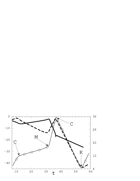
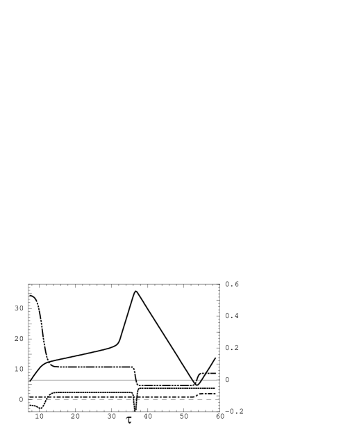
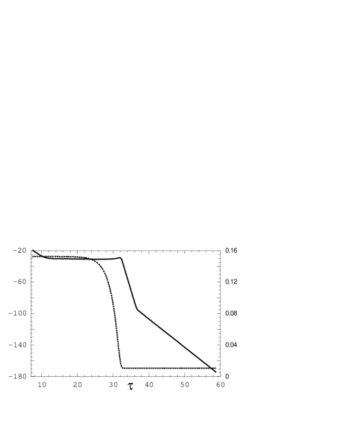
The reason $v$ is so important during a Kasner epoch in determining the next bounce is because $H_{3}/H_{1}$ is controlled by $e^{\lambda+\tau}$ and $H_{2}/H_{1}$ is controlled by $e^{P-\tau}$, and in turn $\lambda+\tau$ and $P-\tau$ are controlled by $v$. In particular, we find that during a Kasner epoch, ${d\lambda/d\tau}\approx-v^{2}$, so that ${d(\lambda+\tau)/d\tau}\approx(1-v^{2})$. Thus if $v<1$, one has $e^{\lambda+\tau}$ increasing exponentially with $\tau$ and therefore ${H_{3}/H_{1}}\to{\cal O}(1)$ in finite time; while if $v>1$, it follows that $\lambda+\tau$ decreases with $\tau$ and $H_{3}/H_{1}$ stays small. The evolution for $P$, governed by ${dP/d\tau}={\pi_{P}/2\pi_{\lambda}}$, is a bit more complicated. However, one finds $-v\leq{dP/d\tau}\leq+v$, so if $v<1$, then ${d(P-\tau)/d\tau}<0$ and $H_{2}/H_{1}$ must decrease. Hence if $v<1$, a magnetic bounce must occur. Now consider the case $v>1$. If $\pi_{P}>0$ and therefore ${dP/d\tau}>0$, then the Kasner evolution leads to ${\pi_{P}/2\pi_{\lambda}}\to v$, and hence ${d(P-\tau)/d\tau}>0$. It follows that ${H_{2}/H_{1}}\to{\cal O}(1)$ in finite time and there is a curvature bounce. If $\pi_{P}<0$ and so ${dP/d\tau}<0$, then the Kasner evolution for $P$ has a single minimum after which $\pi_{P}>0$ and the evolution proceeds to a curvature bounce as just noted. The evolution of $P$ past its minimum is called a kinetic bounce. The kinetic bounce, caused by $e^{-2P}\pi_{Q}^{2}/4\pi_{\lambda}$ in $H_{1}$, keeps $H_{2}$ from dying off in these spacetimes. (See Figs. 1-3.)

What happens after a given bounce occurs? Since, as noted above, a magnetic bounce is essentially a Rosen solution and a curvature bounce is closely approximated by a Taub solution, one can use the known features of those solutions to determine the following [8]. 1) After a magnetic bounce, induced by $v<1$ at $p$, the metric evolution at $p$ returns to a Kasner epoch, this time with $v>1$. A curvature bounce will eventually follow. 2) After a curvature bounce induced by $1<v<3$, one returns to a Kasner epoch with $v<1$, so a magnetic bounce will follow. 3) After a curvature bounce induced by $v>3$, a Kasner epoch occurs with $v>1$, so another curvature bounce will follow.

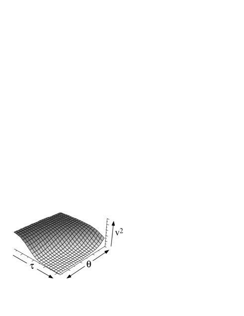
The preceding characterizes the behavior at one point in space. Since $v$, $P$, and $\lambda$ are functions of $\theta$, nearby points will in general not reach the end of a Kasner epoch at exactly the same time. (See Fig. 4.)

There are two different kinds of exceptions to the behavior just described. Neither violates assumption A, but the argument that $H_{2}$ and $H_{3}$ continue to decay and then grow again breaks down in the following ways. First, there exist non-generic spacetimes in the class we are considering which are not Mixmaster. For instance, if we set $B=0$, then $H_{3}$, which causes the magnetic bounces, is missing and these spacetimes will be AVTD.

The second type of exception happens in a generic spacetime, but only at isolated points, not on an open set in the spacetime. There are a number of field configurations that prevent bounces at a point. Some of these have been seen in studies of the Gowdy spacetimes [12]: $Q^{\prime}=0$ when a curvature bounce would normally occur prevents the curvature bounce, and $\pi_{Q}=0$ when a kinetic bounce would normally occur prevents the kinetic bounce (and hence the next curvature bounce if $v>1$). Others are new: $v=1$ during a Kasner epoch prevents both the curvature and magnetic type of bounce and the Kasner epoch persists. If $v=3$ during a Kasner epoch a curvature bounce will occur, but the subsequent Kasner epoch has $v=1$. If $\pi_{P}=0$ during a magnetic bounce the next curvature bounce is prevented. While more and more of these exceptional points occur in a given spacetime as the evolution continues, they will, for generic initial data, always be at isolated values of $\theta$ [20].

Our numerical study, combined with qualitative analysis of the evolution equations, provides strong evidence that, generically, spacetimes in this class exhibit Mixmaster behavior. While this class is spatially inhomogeneous, it is still very restricted. We predict that the particular topology (which determines the boundary conditions on functions of $\theta$) chosen is not necessary and that the generic cosmological spacetime with local 2-torus symmetry and a magnetic field perpendicular to the symmetry directions will also have Mixmaster behavior. But this is still a very restricted class. The question remains whether cosmological spacetimes in general do indeed exhibit Mixmaster behavior, which would be a surprising simplification of their evolution in the neighborhood of the initial singularity, or whether some other possibility in their evolution toward the initial singularity exists [5].

This work was supported in part by a Federal Department of Education Grant to the University of Oregon and by NSF Grants PHY-9308177 to the University of Oregon and PHY-9507313 to Oakland University.

FIG. 1.: Typical evolution at one spatial point. The thick dashed line is $\log_{10}({H_{2}\over H_{1}})$ and the thick solid line is $\log_{10}({H_{3}\over H_{1}})$ (left axis scale). The thin solid line with circles is $P$ (right axis scale). The bounces are labeled. Note that $H_{2}\approx H_{1}$ during the curvature bounces and $H_{3}\approx H_{1}$ during the magnetic bounce. ${H_{2}\over H_{1}}$ starts to grow after the kinetic bounce.

FIG. 2.: Evolution at same spatial point as in Fig. 1. The solid line is $P$ and the dotted line is $\pi_{Q}$ (left axis scale). The dash-single-dotted line is $Q$ and the dash-triple-dotted line is $\pi_{P}$ (right axis scale). Note that $P$ is essentially linear in $\tau$ except during bounces. The other functions are essentially constant for most of the evolution. This graph shows to which type of bounce each function responds.

FIG. 3.: Evolution at the same spatial point as in Figs. 1 and 2. The solid line is $\lambda$ (left axis scale). The dotted line is $\pi_{\lambda}$ (right axis scale). Note that $\lambda$ is essentially linear in $\tau$ except during bounces.

FIG. 4.: This shows $v^{2}$ during the first curvature bounce of Figs. 1-3 with neighboring $\theta$ values included. $v^{2}$ is essentially constant in time during a Kasner epoch and changes during a curvature or a magnetic bounce.

REFERENCES

- [1] E. Kasner, Am. J. Math 43, 217 (1921).
- [2] J. Isenberg and V. Moncrief, Ann. Phys. (N.Y.) 199, 84 (1990).
- [3] D. Eardley, E. Liang, and R. Sachs, J. Math. Phys. 13, 99 (1972).
- [4] The Kasner exponents are the eigenvalues of the extrinsic curvature, divided by the mean curvature. In a Kasner spacetime, the sum of the squares of the Kasner exponents equals one. In a nonvacuum Bianchi I spacetime the sum of the squares of the Kasner exponents is less than one. For examples of cosmological spacetimes which are AVTD but whose evolution toward the singularity does not approach that of a Kasner spacetime see Ref.[9] and A. D. Rendall, J. Math. Phys. 37, 438 (1996).
- [5] There may be other possiblilities. See P. Breitenlohner, G. Lavrelashvili, and D. Maison, gr-qc/9711024; E. E. Donets, D. V. Gal’tsov and M. Yu. Zotov, Phys. Rev. D 56, 3459 (1997).
- [6] V. A. Belinskii, I. M. Khalatnikov, and E. M. Lifshitz, Sov. Phys. Usp. 13, 745 (1971); Adv. Phys. 31, 639 (1982).
- [7] C. W. Misner, Phys. Rev. Lett. 22, 1071 (1969).
- [8] V. G. LeBlanc, D. Kerr, and J. Wainwright, Classical Quantum Gravity 12, 513 (1995).
- [9] J. Wainwright and L. Hsu, Classical Quantum Gravity 6, 1409 (1989).
- [10] A. D. Rendall, Classical Quantum Gravity 14, 2341 (1997); C. G. Hewitt and J. Wainwright, Classical Quantum Gravity 10, 99 (1993).
- [11] B. K. Berger, V. Moncrief, Phys. Rev. D 48, 4676 (1993).
- [12] B. K. Berger and D. Garfinkle, Phys. Rev. D, to be published, gr-qc/9710102.
- [13] B. K. Berger and V. Moncrief, gr-qc/9801078; S. Kichenassamy and A. D. Rendall, Classical Quantum Gravity, to be published; A. D. Rendall, Gen. Relativ. Gravit. 27, 213 (1995); Classical Quantum Gravity 12, 1517 (1995); J. Isenberg and S. Kichenassamy, unpublished; P. T. Chruściel, On Uniqueness in the Large of Solutions of Einstein’s Equations (“Strong Cosmic Censorship”) (Centre for Mathematics and its Applications, Australian National University, Canberra, 1991).
- [14] Relating the ratio between the Hubble time and the Planck time to the logarithm of the spatial volume in a typical Mixmaster evolution shows that, independent of the definition of time, most Mixmaster oscillations occur before the Planck time. However, the spirit of this field of inquiry is to determine the nature of the singularity in classical general relativity. One would expect that, just as in electromagnetism, it will be important to understand the behavior of classical solutions even if a quantum theory of gravity is found.
- [15] Y. Fujiwara, H. Ishihara, and H. Kodama, Classical Quantum Gravity 10, 859 (1993).
- [16] R. Gowdy, Phys. Rev. Lett. 27, 826 (1971); Ann. Phys. (N.Y.) 83, 203 (1974).
- [17] M. Suzuki, Phys. Lett. A 146, 319 (1990).
- [18] A. H. Taub, Ann. Math. 53, 472 (1951).
- [19] G. Rosen, J. Math. Phys. 3, 313 (1962).
- [20] The determination of exactly which spatial point is the exceptional one is delicate. At any given time in the evolution, the function under consideration will vanish (or equal 1) at one value of . The generic behavior is for the function to cross 0 (or 1) in a neighborhood of . The time derivative of that function is very small but nonzero, so the point at which it vanishes will move in time.