Existence theorems for hairy black holes in ${\mathfrak{su}}(N)$ Einstein-Yang-Mills theories.

N.E. Mavromatos^∗ and E. Winstanley
University of Oxford, Theoretical Physics, 1 Keble Road OX1 3NP, U.K.

Abstract
We establish the existence of hairy black holes in ${\mathfrak{su}}(N)$ Einstein-Yang-Mills theories, described by $N-1$ parameters, corresponding to the nodes of the gauge field functions.

PACS numbers: 04.40.Nr, 04.70

December 1997

I Introduction

Interest in non-Abelian Einstein-Yang-Mills theories was sparked by the discovery of particle-like [1] and non-Reissner-Nordström (“hairy”) black hole [2] solutions when the gauge group is ${\mathfrak{su}}(2)$. Since then a plethora of hairy black holes, possessing non-trivial geometry and field structure outside the event horizon, have been found (see, for example, [3]), including coloured black holes in ${\mathfrak{su}}(N)$ Einstein-Yang-Mills theories [4, 5]. Many of these objects have as a fundamental requirement for the existence of hair, a non-Abelian gauge field, often coupled to other fields, such as a Higgs field [6]. As in [6], the existence of gauge hair is not surprising in itself, since the gauge field force is long-range. However, the non-Abelian nature of the field is important for evading the no-hair theorem, for example, for scalar fields coupled to the gauge field. The vast majority of these solutions have been found only numerically, with analytic work in this area at present being limited to an extensive study of the ${\mathfrak{su}}(2)$ case [7, 8, 9], and some analysis of the field equations for general $N$ [10, 11].

In this paper we continue this analysis of the coupled Einstein-Yang-Mills equations for an ${\mathfrak{su}}(N)$ gauge field, and prove analytically the existence of “genuine” hairy black hole solutions for every $N$. By a “genuine” ${\mathfrak{su}}(N)$ black hole, we mean a solution which is not simply the result of embedding a smaller gauge group in ${\mathfrak{su}}(N)$. As in the ${\mathfrak{su}}(2)$ case, the solutions are labeled by the number of nodes of each of the $N-1$ non-zero functions required to describe the gauge field. We shall prove that for each integer $n_{1}$, there are an infinite number of sequences of integers $n_{N-1}\geq n_{N-2}\geq\ldots\geq n_{1}$ corresponding to black hole solutions. It is to be expected that in fact every such sequence corresponds to a black hole solution, but unfortunately we are unable to prove this analytically, although we shall present a numerically-based argument for ${\mathfrak{su}}(3)$ and numerical investigations (such as that done for ${\mathfrak{su}}(5)$ in [4]) for higher dimension groups which indicate that this is in fact the case. The method used to prove the main theorem of this paper is remarkably simple, drawing only on elementary topological ideas.

The structure of the paper is as follows. In section 2 we review briefly the ${\mathfrak{su}}(N)$ Einstein-Yang-Mills field equations and the ansatz and notations we shall employ in the rest of the paper. Next we state some elementary properties of these equations, including results from [11]. The remainder of the paper has a similar progression of ideas as [7], and we continue by first analyzing the behaviour of solutions to the field equations in the two asymptotic regimes, at infinity and close to the event horizon. Although these forms were discussed in [11], we present here a shorter proof. Section 5 is devoted to a discussion of the flat space solutions, which will be important for later propositions. The results here are somewhat weaker than in [7] due to the fact that for ${\mathfrak{su}}(N)$, we have $N-1$ variables and therefore have a $2(N-1)$-dimensional phase space rather than a phase plane as in the ${\mathfrak{su}}(2)$ case, so the powerful Poincaré-Bendixson theory no longer applies. We now consider integrating the field equations outward from the event horizon and consider the various possible behaviours of the resulting solutions. As in [7], there are three types of solution: the regular black holes we are seeking, singular solutions (in which the lapse function vanishes outside the event horizon), and oscillating solutions in which the geometry is not asymptotically flat. The main results of this paper are in sections 7 and 8. An inductive argument is used to prove the existence of solutions for ${\mathfrak{su}}(N)$ assuming existence for ${\mathfrak{su}}(N-1)$ (since we have rigorous theorems for ${\mathfrak{su}}(2)$ [7, 8]). The argument is presented in detail for ${\mathfrak{su}}(3)$ in section 7 and a brief outline of the extension to general $N$ in section 8. Finally, a summary and our conclusions are presented in section 9.

II Ansatz and field equations

In this section we first describe the ansatz we are using and outline the field equations.

The field equations for an ${\mathfrak{su}}(N)$ Yang-Mills gauge field coupled to gravity have been derived in [10] for a spherically symmetric geometry. We take the line element, in the usual Schwarzschild co-ordinates, to be

$$ds^{2}=-S^{2}\mu\,dt^{2}+\mu^{-1}\,dr^{2}+r^{2}\,d\theta^{2}+r^{2}\sin^{2}\theta\,d\phi^{2},$$ (1)

where the metric functions $\mu$ and $S$ are functions of $r$ alone and

$$\mu(r)=1-\frac{2m(r)}{r}.$$ (2)

A spherically symmetric ${\mathfrak{su}}(N)$ gauge potential may be written in the form [10]

$${\cal{A}}=A\,dt+B\,dr+\frac{1}{2}\left(C-C^{H}\right)\,d\theta-\frac{i}{2}\left[\left(C+C^{H}\right)\sin\theta+D\cos\theta\right]\,d\phi$$ (3)

where $D={\mbox{Diag}}\left\{k_{1},k_{2},\ldots,k_{N}\right\}$ with $k_{1}\geq k_{2}\geq\ldots\geq k_{N}$ integers whose sum is zero. In addition, $C$ is a strictly upper triangular complex matrix such that $C_{ij}\neq 0$ only if $k_{i}=k_{j}+2$ and $C^{H}$ its Hermitian conjugate, and $A$, $B$ are anti-Hermitian matrices that commute with $D$. An irreducible representation of ${\mathfrak{su}}(N)$ can be constructed by taking [10]

$$D={\mbox{Diag}}\left\{N-1,N-3,\ldots,-N+3,-N+1\right\}.$$ (4)

In this case $A$, $B$ have trace zero and can be written as

$$A_{jj}=i\left\{-\frac{1}{N}\sum_{k=1}^{j-1}k{\cal{A}}_{k}+\sum_{k=j}^{N-1}\left(1-\frac{k}{N}\right){\cal{A}}_{k}\right\}$$ (5)

for real functions ${\cal{A}}_{k}$, and similarly for $B$. The only non-vanishing entries of $C$ are

$$C_{j,j+1}=\omega_{j}e^{i\gamma_{j}}$$ (6)

where $\omega_{j}$ and $\gamma_{j}$ are real functions. All the functions in this ansatz depend only on $r$. Now we make the following simplifying assumption [10]:

$${\cal{A}}_{j}=0,\qquad{\cal{B}}_{j}+\gamma_{j}^{\prime}=0,\qquad\forall j.$$ (7)

The remaining gauge freedom can then be used to set $B=0$ [12], which implies that the $\gamma_{j}$ are constants, which we choose to be zero for simplicity.

The gauge field equations for the $\omega_{j}$ then take the form [10, 11](where we have set $\kappa=2$ in [10])

$$r^{2}\mu\omega_{j}^{\prime\prime}+\left(2m-2r^{3}p_{\theta}\right)\omega_{j}^{\prime}+\left[1-\omega_{j}^{2}+\frac{1}{2}\left(\omega_{j-1}^{2}+\omega_{j+1}^{2}\right)\right]\omega_{j}=0,$$ (8)

where

$$p_{\theta}=\frac{1}{4r^{4}}\sum_{j=1}^{N}\left[\omega_{j}^{2}-\omega_{j-1}^{2}-N-1+2j\right]^{2}$$ (9)

and the Einstein equations can be simplified to

$$m^{\prime}=\mu G+r^{2}p_{\theta},\qquad\frac{S^{\prime}}{S}=\frac{2G}{r}$$ (10)

where

$$G=\sum_{j=1}^{N-1}\omega_{j}^{{}^{\prime}2}.$$ (11)

Note that $\omega_{0}\equiv 0\equiv\omega_{N}$, so that these are the usual equations [2] in the ${\mathfrak{su}}(2)$ case, and have a very similar, but slightly coupled, structure for general $N$. The equations (8–11) possess two symmetries [11]. Firstly, the substitution $\omega_{j}\rightarrow-\omega_{j}$ for any fixed $j$ leaves the equations invariant, exactly as in the ${\mathfrak{su}}(2)$ case. Secondly, there is an additional symmetry under the transformation $j\rightarrow N-j$ for all $j$. We will not assume that this symmetry is respected by the solutions of the field equations, so that the ${\mathfrak{su}}(3)$ case is not necessarily trivial.

We are concerned in this paper with black holes, which will have a regular event horizon at $r=r_{h}$, where $\mu=0$. The equations in their present form are singular at $r_{h}$, so in order to produce a set of equations which are regular as $\mu\rightarrow 0$, we define a new independent variable $\tau$ by [7]

$$\frac{dr}{d\tau}=r{\sqrt{\mu}},$$ (12)

denote $d/d\tau$ by ${\dot{}}$, and define new dependent variables $\kappa$, $U_{j}$ and $\Psi$ as follows [7]:

$$\Psi={\sqrt{\mu}},\qquad U_{j}=\Psi\omega_{j}^{\prime},\qquad\kappa=\frac{1}{2\Psi}\left(1+\Psi^{2}+2\mu G-2r^{2}p_{\theta}\right).$$ (13)

Then the field equations take the form [7]:

$${\dot{r}} = r\Psi$$ (14)

$${\dot{\omega}}_{j} = rU_{j}$$ (15)

$${\dot{\Psi}} = \left(\kappa-\Psi\right)\Psi-2\mu G$$ (16)

$$\left(S\Psi\right){\dot{}} = S\left(\kappa-\Psi\right)\Psi$$ (17)

$${\dot{U}}_{j} = -\left(\kappa-\Psi\right)U_{j}-\frac{1}{r}\left[1-\omega_{j}^{2}+\frac{1}{2}\left(\omega_{j+1}^{2}+\omega_{j-1}^{2}\right)\right]\omega_{j}$$ (18)

$${\dot{\kappa}} = -\kappa^{2}+1+2\mu G.$$ (19)

The main thrust of this article is to prove the existence of regular, black hole, solutions of the field equations for general $N$ with $N-1$ degrees of freedom. In other words, we begin with a regular event horizon at $r=r_{h}$, where $\mu=0$, and integrate outwards with increasing $r$. Later we shall classify the possible behaviour of the solutions as $r$ increases. We are interested primarily in those solutions which possess the physical properties of a black hole geometry, namely for which $\mu>0$ for all $r>r_{h}$, the $\omega_{j}$ and their derivatives are finite for all $r>r_{h}$ and the spacetime becomes flat in the limit $r\rightarrow\infty$. We shall refer to such solutions as regular black hole solutions.

III Elementary results

In this this section we state a few elementary results, which will prove useful in later analysis. Firstly, two lemmas which are proved in the ${\mathfrak{su}}(N)$ case exactly as in the ${\mathfrak{su}}(2)$ case, see [7].

Lemma III.1

If $\mu(r_{0})<1$ for some $r_{0}$ then $\mu(r)<1$ for all $r\geq r_{0}$.

Lemma III.2

As long as $0<\mu<1$ all field variables are regular functions of $r$.

These two lemmas show that for a regular event horizon at $r=r_{h}$, where $\mu=0$, then $\mu<1$ for all $r>r_{h}$ and the field variables are regular functions as long as $\mu>0$. The black hole solutions we seek approach the Schwarzschild geometry as $r\rightarrow\infty$, so we may assume that all $\omega_{j}$ are bounded for all $r$ (from lemma III.2 each $\omega_{j}$ is bounded on every closed interval $[r_{h},r_{1}]$, so we are simply assuming that $\omega_{j}$ remains bounded as $r\rightarrow\infty$). It will be proved in section VI that this assumption is in fact valid for solutions having $\mu>0$ for all $r$. Define a quantity $M_{j}$ for each $j$ to be the lowest upper bound on $\omega_{j}^{2}$, i.e.

$$\omega_{j}^{2}\leq M_{j},\qquad\forall j=1,2,\ldots,N-1.$$ (20)

It has been shown in [8] that the following result is true for $N=2$, and proved in general with the assumption that all $\omega_{j}$ are bounded via an elegant method in [11].

Theorem III.3

$M_{j}\leq j(N-j)$.

Part of the proof of this theorem in [11] involves a knowledge of where $\omega_{j}$ may have maxima or minima. The result following is less powerful than in the ${\mathfrak{su}}(2)$ case due to the coupling in the gauge field equation (8).

Proposition III.4

As long as $\mu(r)>0$, the function $\omega_{j}(r)$ cannot have maxima in the regions

$$\omega_{j}>{\sqrt{1+\frac{1}{2}\left(\omega_{j+1}^{2}+\omega_{j-1}^{2}\right)}}\qquad{\mbox{and}}\qquad 0>\omega_{j}>-{\sqrt{1+\frac{1}{2}\left(\omega_{j+1}^{2}+\omega_{j-1}^{2}\right)}}$$ (21)

or minima in the regions

$$\omega_{j}<-{\sqrt{1+\frac{1}{2}\left(\omega_{j+1}^{2}+\omega_{j-1}^{2}\right)}}\qquad{\mbox{and}}\qquad 0<\omega_{j}<{\sqrt{1+\frac{1}{2}\left(\omega_{j+1}^{2}+\omega_{j-1}^{2}\right)}}.$$ (22)

Proof
When $\omega_{j}^{\prime}=0$, from (8),

$$\mu\omega_{j}^{\prime\prime}=-\frac{1}{r^{2}}\left[1-\omega_{j}^{2}+\frac{1}{2}\left(\omega_{j+1}^{2}+\omega_{j-1}^{2}\right)\right]\omega_{j},$$ (23)

so that $\omega_{j}$ will have a maximum if

$$\omega_{j}>0\qquad{\mbox{and}}\qquad\omega_{j}^{2}<1+\frac{1}{2}\left(\omega_{j+1}^{2}+\omega_{j-1}^{2}\right)$$ (24)

or

$$\omega_{j}<0\qquad{\mbox{and}}\qquad\omega_{j}^{2}>1+\frac{1}{2}\left(\omega_{j+1}^{2}+\omega_{j-1}^{2}\right).$$ (25)

Similarly, $\omega_{j}$ will have a minimum if

$$\omega_{j}>0\qquad{\mbox{and}}\qquad\omega_{j}^{2}>1+\frac{1}{2}\left(\omega_{j+1}^{2}+\omega_{j-1}^{2}\right)$$ (26)

or

$$\omega_{j}<0\qquad{\mbox{and}}\qquad\omega_{j}^{2}<1+\frac{1}{2}\left(\omega_{j+1}^{2}+\omega_{j-1}^{2}\right).$$ (27)

$\square$

IV Asymptotic behaviour of solutions

We seek solutions to the above field equations representing black holes with a regular event horizon at $r=r_{h}$ and finite total energy density. In order to prove the local existence of solutions of the field equations with the desired asymptotic behaviour, we shall apply the following theorem [7].

Theorem IV.1

Consider a system of differential equations for $n+m$ functions ${\mbox{\boldmath{$a$}}}=(a_{1},a_{2},\ldots,a_{n})$ and ${\mbox{\boldmath{$b$}}}=(b_{1},b_{2},\ldots,b_{m})$ of the form

$$x\frac{da_{i}}{dx} = x^{p_{i}}f_{i}(x,{\mbox{\boldmath{$a$}}},{\mbox{\boldmath{$b$}}}),$$

$$x\frac{db_{i}}{dx} = -\lambda_{i}b_{i}+x^{q_{i}}g_{i}(x,{\mbox{\boldmath{$a$}}},{\mbox{\boldmath{$b$}}}),$$ (28)

with constants $\lambda_{i}>0$ and integers $p_{i},q_{i}\geq 1$ and let ${\cal{C}}$ be an open subset of ${\mathbb{R}}^{n}$ such that the functions $f_{i}$ and $g_{i}$ are analytic in a neighbourhood of $x=0$, ${\mbox{\boldmath{$a$}}}={\mbox{\boldmath{$c$}}}$, ${\mbox{\boldmath{$b$}}}={\mbox{\boldmath{$0$}}}$, for all ${\mbox{\boldmath{$c$}}}\in{\cal{C}}$. Then there exists an $n$-parameter family of solutions of the system (28) such that

$$a_{i}(x)=c_{i}+O(x^{p_{i}}),\qquad b_{i}(x)=O(x^{q_{i}}),$$ (29)

where $a_{i}(x)$ and $b_{i}(x)$ are defined for ${\mbox{\boldmath{$c$}}}\in{\cal{C}}$, and $|x|<x_{0}({\mbox{\boldmath{$c$}}})$ and are analytic in $x$ and $c$.

In this section we consider only the equations for $\mu$ and the $\omega_{j}$. The equation for $S$ (10) is independent of the others and hence can be integrated immediately once we have the other field variables, with an additional parameter. This procedure gives a finite answer on any closed, bounded interval on which the remaining variables are finite. Results similar to propositions IV.2 and IV.3 were proved in [11], but here we are using a more straightforward approach.

A Behaviour at infinity

As $r\rightarrow\infty$, in order to have finite total energy density, the geometry must approach the Schwarzschild solution, that is

$$m\rightarrow M={\mbox{constant}},\qquad G\rightarrow 0,\qquad p_{\theta}\rightarrow 0.$$ (30)

Hence each $\omega_{j}$ must approach a constant value, which is fixed by (30) to be

$$\omega_{j}^{2}\rightarrow j(N-j).$$ (31)

The equations for the $\omega_{j}$ are then automatically satisfied in the limit as $r\rightarrow\infty$.

Proposition IV.2

There exists an $N$-parameter family of local solutions of (8–11) near $r=\infty$ analytic in $c_{j}$, $M$ and $r^{-1}$ such that

$$\mu(r) = 1-\frac{2M}{r}+O\left(\frac{1}{r^{4}}\right)$$

$$\omega_{j}(r) = {\sqrt{j(N-j)}}-\frac{c_{j}}{r}+O\left(\frac{1}{r^{2}}\right).$$ (32)

Proof
Introduce new variables

$$x=\frac{1}{r},\qquad\psi_{j}=r\left({\sqrt{j(N-j)}}-\omega_{j}\right),\qquad\xi_{j}=r^{2}\mu\omega_{j}^{\prime}\qquad\lambda=r\left(1-\mu\right).$$ (33)

Then

$$x\frac{d\lambda}{dx}=-\frac{2}{x}\left(\mu G+r^{2}p_{\theta}\right)$$ (34)

where

$$G=x^{4}\sum_{j=1}^{N-1}\frac{\xi_{j}^{2}}{\mu^{2}}$$ (35)

and

$$p_{\theta} = \frac{x^{4}}{4}\sum_{j=1}^{N}\left[x^{2}\psi_{j}^{2}-x^{2}\psi_{j-1}^{2}-2x\psi_{j}{\sqrt{j(N-j)}}\right.$$ (36)

$$\left.+2x\psi_{j-1}{\sqrt{(j-1)(N-j+1)}}\right]^{2},$$

that is,

$$x\frac{d\lambda}{dx}=-x^{3}f_{\lambda}$$ (37)

where $f_{\lambda}$ is a polynomial in $x$, $\mu^{-1}$, $\xi$’s and $\psi$’s. Similarly,

$$x\frac{d\psi_{j}}{dx}=-\psi_{j}+\frac{1}{\mu}\xi_{j}=-\psi_{j}+\xi_{j}+xf_{\psi_{j}}$$ (38)

where $f_{\psi_{j}}$ is analytic in $x$, $\lambda$, $\psi$’s and $\xi$’s in a neighbourhood of $x=0$. Using the field equations we also have

$$x\frac{d\xi_{j}}{dx} = -2\xi_{j}+2\psi_{j}\left[j(N-j)\right]-\psi_{j-1}{\sqrt{j(j-1)(N-j)(N-j+1)}}$$ (39)

$$-\psi_{j+1}{\sqrt{j(j+1)(N-j)(N-j-1)}}+xf_{\xi_{j}}$$

where $f_{\xi_{j}}$ is a polynomial in $x$, $\mu^{-1}$, $\psi$’s and $\xi$’s. The algebra simplifies if we define new functions $\alpha_{j}$, $\beta_{j}$ such that

$$\psi_{j} = \alpha_{j}+\beta_{j}$$

$$\xi_{j} = \alpha_{j}+\Lambda\beta_{j}$$ (40)

where $\Lambda$ is a real constant not equal to unity. The equations for $\alpha_{j}$ and $\beta_{j}$ then read

$$(\Lambda-1)x\frac{d\alpha_{j}}{dx} = 2\alpha_{j}-2[j(N-j)]\alpha_{j}+{\sqrt{j(j-1)(N-j)(N-j+1)}}\alpha_{j-1}$$

$$+{\sqrt{j(j+1)(N-j)(N-j-1)}}\alpha_{j+1}+(\Lambda^{2}+\Lambda)\beta_{j}$$

$$-2[j(N-j)]\beta_{j}+{\sqrt{j(j-1)(N-j)(N-j+1)}}\beta_{j-1}$$

$$+{\sqrt{j(j+1)(N-j)(N-j-1)}}\beta_{j+1}+xf_{\alpha_{j}}$$

$$(\Lambda-1)x\frac{d\beta_{j}}{dx} = -2\alpha_{j}+2[j(N-j)]\alpha_{j}-{\sqrt{j(j-1)(N-j)(N-j+1)}}\alpha_{j-1}$$ (41)

$$-{\sqrt{j(j+1)(N-j)(N-j-1)}}\alpha_{j+1}+(1-3\Lambda)\beta_{j}$$

$$+2[j(N-j)]\beta_{j}-{\sqrt{j(j-1)(N-j)(N-j+1)}}\beta_{j-1}$$

$$-{\sqrt{j(j+1)(N-j)(N-j-1)}}\beta_{j+1}+xf_{\beta_{j}},$$

where the $f_{\alpha_{j}}$ and $f_{\beta_{j}}$ are analytic functions of $x$, $\mu^{-1}$, $\alpha$’s and $\beta$’s. Consider the matrix ${\cal{M}}_{N-1}$ whose entries are

$$\left(\begin{array}[]{ccc}2(N-1)&-{\sqrt{(N-1)2(N-2)}}&\ldots\\ -{\sqrt{(N-1)2(N-2)}}&2.2(N-2)&\ldots\\ 0&-{\sqrt{2(N-2)3(N-3)}}&\ldots\\ \vdots&\vdots&\vdots\\ \end{array}\right).$$ (42)

For a vector ${\mbox{\boldmath{$q$}}}=\left(q_{1},\ldots,q_{N-1}\right)$, let $p_{j}={\sqrt{j(N-j)}}q_{j}$ for $j=1,\ldots,N-1$. Then

$${\mbox{\boldmath{$q$}}}^{T}{\cal{M}}_{N-1}{\mbox{\boldmath{$q$}}}=p_{1}^{2}+p_{N-1}^{2}+\left(p_{1}-p_{2}\right)^{2}+\ldots\left(p_{N-2}-p_{N-1}\right)^{2}.$$ (43)

Hence the matrix ${\cal{M}}_{N-1}$ is real, symmetric and positive definite, and will have positive real eigenvalues ${\cal{E}}_{i}$, and corresponding eigenvectors ${\mbox{\boldmath{$v$}}}_{i}$. We may expand our variable vectors in terms of eigenvectors of ${\cal{M}}_{N-1}$ as follows:

$${\mbox{\boldmath{$\alpha$}}}=\sum_{i=1}^{N-1}A_{i}(x){\mbox{\boldmath{$v$}}}_{i}\qquad{\mbox{\boldmath{$\beta$}}}=\sum_{i=1}^{N-1}B_{i}(x){\mbox{\boldmath{$v$}}}_{i}$$ (44)

$${\mbox{\boldmath{$f$}}}_{\alpha}=\sum_{i=1}^{N-1}F_{i}(x){\mbox{\boldmath{$v$}}}_{i}\qquad{\mbox{\boldmath{$f$}}}_{\beta}=\sum_{i=1}^{N-1}G_{i}(x){\mbox{\boldmath{$v$}}}_{i},$$ (45)

in terms of which the equations (41) now become:

$$(\Lambda-1)x\frac{dA_{i}}{dx} = (2-{\cal{E}}_{i})A_{i}+(\Lambda^{2}+\Lambda-{\cal{E}}_{i})B_{i}+xF_{i}$$

$$(\Lambda-1)x\frac{dB_{i}}{dx} = ({\cal{E}}_{i}-2)A_{i}+(1-3\Lambda+{\cal{E}}_{i})B_{i}+xG_{i}.$$ (46)

This transformation has removed the coupling between the $j$’s but the $A$’s and $B$’s are still coupled. Repeating the procedure with the matrix ${\cal{P}}_{i}$ will decouple these equations, where

$${\cal{P}}_{i}=\left(\begin{array}[]{cc}2-{\cal{E}}_{i}&\Lambda^{2}+\Lambda-{\cal{E}}_{i}\\ -2+{\cal{E}}_{i}&1-3\Lambda+{\cal{E}}_{i}\end{array}\right).$$ (47)

This matrix has eigenvalues

$$\mu_{\pm}=\frac{1}{2}(1-\Lambda)\left(3\pm{\sqrt{1+4{\cal{E}}_{i}}}\right)$$ (48)

and corresponding eigenvectors ${\mbox{\boldmath{$V$}}}_{\pm}$. Writing

$$\left(\begin{array}[]{c}A_{i}\\ B_{i}\end{array}\right)=C_{+}(x){\mbox{\boldmath{$V$}}}_{+}+C_{-}(x){\mbox{\boldmath{$V$}}}_{-},\qquad\left(\begin{array}[]{c}F_{i}\\ G_{i}\end{array}\right)=D_{+}(x){\mbox{\boldmath{$V$}}}_{+}+D_{-}(x){\mbox{\boldmath{$V$}}}_{-},$$ (49)

the equations are now

$$(\Lambda-1)x\frac{dC_{\pm}}{dx}=\mu_{\pm}C_{\pm}+xD_{\pm}.$$ (50)

In the case where $\mu_{-}<0$, theorem IV.1 applies directly and we have

$$C_{-}=O(x);$$ (51)

when $\mu_{-}=0$ (corresponding to ${\cal{E}}_{i}=2$),

$$C_{-}=K_{-}+O(x)$$ (52)

for some constant $K_{-}$. The other eigenvalue $\mu_{+}$ is always strictly positive, and in this situation theorem IV.1 does not apply. However, equation (50) can be integrated using the standard Picard method (see, for example, [13]) to give an analytic solution

$$C_{+}=K_{+}+O(x).$$ (53)

Both $C_{\pm}$ will be analytic in $K_{\pm}$ and $x$ in some neighbourhood of $x=0$ and substituting back through equations (44,49) gives solutions of the form (32) as required. $\square$

B Behaviour at the event horizon

We assume that at $r=r_{h}$ there is a non-degenerate event horizon, namely $\mu(r_{h})=0$, but $\mu^{\prime}(r_{h})>0$ is finite.

Proposition IV.3

There exists an $N$-parameter family of local solutions of (8–11) near $r=r_{h}$, analytic in $r_{h}$, $\omega_{j,h}$ and $r$ such that

$$\mu(r_{h}+\rho) = \mu^{\prime}(r_{h})+O(\rho),$$

$$\omega_{j}(r_{h}+\rho) = \omega_{j,h}+\omega_{j}^{\prime}(r_{h})+O(\rho^{2})$$ (54)

where $\mu^{\prime}(r_{h})$ and $\omega_{j}^{\prime}(r_{h})$ are functions of the $\omega_{j,h}$.

Proof
Let $\rho=r-r_{h}$ be the new independent variable, and define

$$x=r,\qquad\lambda=\frac{\mu}{\rho},\qquad\psi_{j}=\omega_{j},\qquad\xi_{j}=\frac{\mu\omega_{j}^{\prime}}{\rho}.$$ (55)

Then the field equations take the form

$$\rho\frac{dx}{d\rho} = \rho,$$ (56)

$$\rho\frac{d\lambda}{d\rho} = -\lambda+\left[\frac{1}{x}-2xp_{\theta}\right]+\rho\frac{\lambda}{x}\left[1-2G\right]$$ (57)

$$= -\lambda+\rho H_{\lambda}+F_{\lambda}$$

$$\rho\frac{d\psi_{j}}{d\rho} = \frac{\rho\xi_{j}}{\lambda}$$ (58)

$$\rho\frac{d\xi_{j}}{d\rho} = -\xi_{j}+\rho H_{j}+F_{j},$$ (59)

where the $F$’s and $H$’s are polynomials in $x^{-1}$, $\lambda^{-1}$, and the other variables, and the $F$’s depend only on $x$ and $\psi_{j}$’s. Next define

$${\tilde{\xi}}_{j}=\xi_{j}-F_{j},\qquad{\tilde{\lambda}}=\lambda-F_{\lambda},$$ (60)

whose derivatives are given by

$$\rho\frac{d{\tilde{\xi}}_{j}}{d\rho} = -{\tilde{\xi}}_{j}+\rho G_{j}$$ (61)

$$\rho\frac{d{\tilde{\lambda}}}{d\rho} = -{\tilde{\lambda}}+\rho G_{\lambda}.$$ (62)

Here the $G$’s are analytic in $x^{-1}$, $\lambda^{-1}$, $\lambda$, $x$, ${\tilde{\lambda}}$, $\psi_{j}$, ${\tilde{\xi}}_{j}$. Applying theorem IV.1, there exist solutions of the form

$$x=r_{h}+\rho,\qquad\psi_{j}=\omega_{j,h}+O(\rho),\qquad{\tilde{\lambda}},{\tilde{\xi}}_{j}=O(\rho),$$ (63)

which gives the behaviour (54), together with the required analyticity. From the field equations (8–11), setting $\mu(r_{h})=0$ gives the following relations:

$$\mu^{\prime}(r_{h}) = \frac{1}{2}r_{h}^{2}p_{\theta}(r_{h})$$ (64)

$$\omega_{j}^{\prime}(r_{h}) = -\frac{\left[1-\omega_{j,h}^{2}+\frac{1}{2}\left(\omega_{j-1,h}^{2}+\omega_{j+1,h}^{2}\right)\omega_{j,h}\right]}{r_{h}-r_{h}^{3}p_{\theta}(r_{h})}$$ (65)

where

$$p_{\theta}(r_{h})=\frac{1}{4r_{h}^{4}}\sum_{j=1}^{N}\left[\omega_{j,h}^{2}-\omega_{j-1,h}^{2}-N-1+2j\right]^{2}.$$ (66)

$\square$

V Flat space solutions

The behaviour of the gauge field equations in the flat space limit will be useful later in section VI when we come to examine the properties of regular solutions. We are not concerned here with the global existence of flat space solutions but only the local properties pertinent to the curved space problem.

The analysis here is similar to that in [7], but note that for general $N$ there will be $N-1$ coupled gauge field equations. The powerful Poincaré-Bendixson theory of autonomous systems is not applicable when $N>2$, and so we will be able to derive only correspondingly weaker results, and cannot draw a phase portrait. Fortunately the theorems later require only a knowledge of the nature of the critical points and the local behaviour close to these points, which is the subject of this section.

In flat space the gauge field equations reduce to:

$$r^{2}\omega_{j}^{\prime\prime}+\left[1-\omega_{j}^{2}+\frac{1}{2}\left(\omega_{j+1}^{2}+\omega_{j-1}^{2}\right)\right]\omega_{j}=0.$$ (67)

These equations can be made autonomous by changing variables to $\tau=\log r$, and denoting $d/d\tau$ by ${\dot{}}$:

$${\ddot{\omega}}_{j}-{\dot{\omega}}_{j}+\left[1-\omega_{j}^{2}+\frac{1}{2}\left(\omega_{j+1}^{2}+\omega_{j-1}^{2}\right)\right]\omega_{j}=0.$$ (68)

This system of $N-1$ coupled equations has critical points when

$$\left[1-\omega_{j}^{2}+\frac{1}{2}\left(\omega_{j+1}^{2}+\omega_{j-1}^{2}\right)\right]\omega_{j}=0.\qquad\forall j=1,2,\ldots,N-1.$$ (69)

If $\omega_{j}\neq 0$ for all $j$ then

$$\omega_{j}={\sqrt{j(N-j)}}.$$ (70)

There is also a critical point when $\omega_{j}=0$ for all $j$.

The other critical points can be described as follows. Suppose that $\omega_{i}=0$ and $\omega_{i+k}=0$ but that $\omega_{i+m}\neq 0$ for $m=1,\ldots,k-1$ (where $k\geq 2$). The critical point is then described by the equations

$$0 = \omega_{i}$$

$$0 = 1-\omega_{i+1}^{2}+\frac{1}{2}\left(\omega_{i}^{2}+\omega_{i+2}^{2}\right)$$

$$\vdots$$

$$0 = 1-\omega_{i+k-1}^{2}+\frac{1}{2}\left(\omega_{i+k-2}^{2}+\omega_{i+k}^{2}\right)$$

$$0 = \omega_{i+k}$$ (71)

which have the solution

$$\omega_{i+m}={\sqrt{m(k-m)}}\qquad{\mbox{for $m=1,\ldots,k-1$}}.$$ (72)

In other words, if we have a run of $k$ non-zero $\omega$’s with zero $\omega_{i}$ at each end, then the solution for the non-zero $\omega$’s is the same as the $N=k$ case with no zero $\omega$’s. We can also put together a run of as many zero $\omega$’s as we like in the critical point.

In order to classify the critical points, we linearize the field equations. Let

$$\omega_{j}(\tau)=\omega_{j}^{(0)}+\epsilon_{j}(\tau)$$ (73)

where $\omega_{j}^{(0)}$ is the value of $\omega_{j}$ at the critical point and $\epsilon_{j}$ is a small perturbation. The equation for $\epsilon_{j}$ is, to first order,

$$0 = {\ddot{\epsilon}}_{j}-{\dot{\epsilon}}_{j}+\epsilon_{j}\left[1-\omega_{j}^{(0)2}+\frac{1}{2}\left(\omega_{j+1}^{(0)2}+\omega_{j-1}^{(0)2}\right)\right]$$ (74)

$$+\omega_{j}^{(0)}\left[-2\epsilon_{j}\omega_{j}^{(0)}+\epsilon_{j+1}\omega_{j+1}^{(0)}+\epsilon_{j-1}\omega_{j-1}^{(0)}\right].$$

We shall take the two cases we need to consider in turn.

Firstly, the case where $\omega_{j}^{(0)}=0$, when the equation for $\epsilon_{j}$ reduces to

$${\ddot{\epsilon}}_{j}-{\dot{\epsilon}}_{j}+\epsilon_{j}\left[1+\frac{1}{2}\left(\omega_{j+1}^{(0)2}+\omega_{j-1}^{(0)2}\right)\right]=0.$$ (75)

In order to find the nature of the critical point, let

$$\epsilon_{j}=e^{\lambda\tau},$$ (76)

then $\lambda$ satisfies the equation

$$\lambda^{2}-\lambda+\left[1+\frac{1}{2}\left(\omega_{j+1}^{(0)2}+\omega_{j-1}^{(0)2}\right)\right]=0.$$ (77)

This implies that

$$\lambda=\frac{1}{2}\pm\frac{1}{2}i\alpha,$$ (78)

where $\alpha$ is the positive real number given by

$$\alpha^{2}=3+2\omega_{j+1}^{(0)2}+2\omega_{j-1}^{(0)2}.$$ (79)

We conclude that, in the $(\epsilon_{j},{\dot{\epsilon}}_{j})$ plane, we have an unstable focal point, as found in the ${\mathfrak{su}}(2)$ case in [7].

Secondly, we consider the situation in which there is at least one $\omega_{j}^{(0)}$ which is non-zero. Suppose that $\omega_{i}^{(0)}=0$, and $\omega_{i+k}^{(0)}=0$, but $\omega_{i+m}^{(0)}\neq 0$ for $m=1,\ldots,k-1$, where we include the case that $i=0$ and $k=N$. Then we have a series of coupled perturbation equations:

$$0 = {\ddot{\epsilon}}_{i+1}-{\dot{\epsilon}}_{i+1}-2\epsilon_{i+1}\omega_{i+1}^{(0)2}+\epsilon_{i+2}\omega_{i+2}^{(0)}\omega_{i+1}^{(0)}$$

$$0 = {\ddot{\epsilon}}_{i+2}-{\dot{\epsilon}}_{i+2}-2\epsilon_{i+2}\omega_{i+2}^{(0)2}+\epsilon_{i+3}\omega_{i+3}^{(0)}\omega_{i+2}^{(0)}+\epsilon_{i+1}\omega_{i+1}^{(0)}\omega_{i+2}^{(0)}$$

$$\vdots$$

$$0 = {\ddot{\epsilon}}_{i+k-1}-{\dot{\epsilon}}_{i+k-1}-2\epsilon_{i+k-1}\omega_{i+k-1}^{(0)2}+\epsilon_{i+k-2}\omega_{i+k-2}^{(0)}\omega_{i+k-1}^{(0)}.$$ (80)

Define a vector $\epsilon$ by

$${\mbox{\boldmath{$\epsilon$}}}=\left(\epsilon_{i+1},\ldots,\epsilon_{i+k-1}\right)^{T}$$ (81)

and consider solutions of the form

$${\mbox{\boldmath{$\epsilon$}}}=e^{\lambda\tau}{\mbox{\boldmath{$q$}}}$$ (82)

where $q$ is a constant vector. Then $\lambda^{2}-\lambda$ are eigenvalues of the matrix ${\cal{M}}_{k-1}$ given by (42). As discussed in section IV, the matrix ${\cal{M}}_{k-1}$ has positive real eigenvalues ${\cal{E}}_{j}$. Then

$$\lambda=\frac{1\pm{\sqrt{1+4{\cal{E}}_{j}}}}{2}=j+1,-j$$ (83)

will have positive and negative real values and there is a saddle point. Again this is in direct analogy with the ${\mathfrak{su}}(2)$ case [7].

VI Global behaviour of the solutions

In this section we investigate the behaviour of solutions of the regular field equations (14–19) as functions of $\tau$. From section IV, we know that, given any starting values $\omega_{j,h}$ for the gauge field functions, then there is a local solution of the field equations in a neighbourhood of the regular event horizon at $r=r_{h}$, $\tau=0$, which is analytic in $\tau$ and the initial parameters. Furthermore, from lemma III.2 as long as $0<\Psi<1$ the solutions remain regular. Therefore, as we integrate out in $\tau$ from the event horizon there are only three possibilities:

1. There is a $\tau_{0}>0$ such that $\Psi(\tau_{0})=0$.

2. For all $\tau>0$, we have $\Psi(\tau)>0$ and $r(\tau)$ remains bounded as $\tau\rightarrow\infty$.

3. For all $\tau>0$, we have $\Psi(\tau)>0$ and $r(\tau)\rightarrow\infty$ as $\tau\rightarrow\infty$.

We refer to solutions of the first type as singular solutions. Those of type 2 are known as oscillating solutions in [7] and we retain their terminology. It will be shown below (proposition VI.4), that there is a maximum value $r_{max}$ of $r$ for oscillating solutions. Finally, we denote by $S_{\infty}$ solutions of the first type for which $r(\tau_{0})<r_{max}$. Our first task is to show that solutions of type 3 are precisely the black hole solutions we are seeking. We begin by proving the assumption made at the end of section II, namely that for solutions of type 3, each $\omega_{j}$ is bounded for all $r$.

Lemma VI.1

If $\Psi(\tau)>0$ for all $\tau$ and $\lim_{\tau\rightarrow\infty}r(\tau)=\infty$ then all the $\omega_{j}$ remain bounded as $r\rightarrow\infty$.

Proof
From the local existence propositions IV.3 and IV.2 and lemma III.2, each $\omega_{j}$ is an analytic function of $r$ as long as $\mu>0$. Introduce a new variable $x=r^{-1}$, then each $\omega_{j}$ is an analytic function of $x$ in a neighbourhood of $x=0$, except possibly at $x=0$, and can be written as a Laurent series:

$$\omega_{j}(x)=\sum_{n=-\infty}^{\infty}a_{n}^{j}x^{n}.$$ (84)

In order for $\mu>0$ for all $r$, it must be the case that $2mr^{-1}=2mx<1$, although $m$ itself need not necessarily remain bounded. Hence $2mx$ is bounded in a neighbourhood of $x=0$, and in particular is analytic at $x=0$. Therefore we can write

$$2mx=\sum_{n=0}^{\infty}b_{n}x^{n}.$$ (85)

Thus

$$m=\frac{1}{2}\sum_{n=0}^{\infty}b_{n}x^{n-1},\qquad\frac{dm}{dr}=-x^{2}\frac{dm}{dx}=-\frac{1}{2}\sum_{n=0}^{\infty}b_{n}(n-1)x^{n},$$ (86)

so that $dm/dr$ is analytic in a neighbourhood of $x=0$. From the field equations,

$$\frac{dm}{dr}=\mu G+r^{2}p_{\theta}$$ (87)

where

$$G=\sum_{j=1}^{N-1}\left(\frac{d\omega_{j}}{dr}\right)^{2}\qquad r^{2}p_{\theta}=\frac{x^{2}}{4}\sum_{j=1}^{N}\left[\omega_{j}^{2}-\omega_{j-1}^{2}-N-1+2j\right]^{2}.$$ (88)

Since both $G$ and $r^{2}p_{\theta}$ are positive, they must each be analytic in a neighbourhood of $x=0$. Consider $G$ first, using

$$\frac{d\omega_{j}}{dr}=-x^{2}\frac{d\omega_{j}}{dx}=-\sum_{n=-\infty}^{\infty}a_{n}^{j}nx^{n+1}$$ (89)

and since $\left(\frac{d\omega_{j}}{dr}\right)^{2}$ must be analytic near $x=0$, it must be the case that

$$a_{n}^{j}=0\qquad\forall n<-1.$$ (90)

Then

$$\omega_{j}^{2}=\frac{a_{-1}^{j2}}{x^{2}}+\sum_{n=-1}^{\infty}c_{n}^{j}x^{n}$$ (91)

for constants $c_{n}^{j}$ and hence

$$\omega_{j}^{2}-\omega_{j-1}^{2}-N-1+2j=\frac{1}{x^{2}}\left[a_{-1}^{j2}-a_{-1}^{(j-1)2}\right]+\sum_{n=-1}^{\infty}d_{n}^{j}x^{n}.$$ (92)

Since $r^{2}p_{\theta}$ is analytic,

$$a_{-1}^{j}=\pm a_{-1}^{j-1}\qquad\forall j.$$ (93)

But $\omega_{0}\equiv 0$, so $a_{-1}^{0}=0$ and thus $a_{-1}^{j}=0$ for all $j$. We conclude that $\omega_{j}$ is analytic at $x=0$, and therefore finite as $x=0$. Therefore $\omega_{j}$ is bounded for all $r\in[r_{h},\infty)$. $\square$

Proposition VI.2

If $\Psi(\tau)>0$ for all $\tau$ and $\lim_{\tau\rightarrow\infty}r(\tau)=\infty$ then the solution tends to one of the flat space critical points, with the exception of the origin.

The proof of this proposition closely follows Proposition 14 of Ref. 7, the main thrust of which is the following lemma.

Lemma VI.3

If $\Psi(\tau)>0$ for all $\tau$ and $\lim_{\tau\rightarrow\infty}r(\tau)=\infty$ then

$$\lim_{\tau\rightarrow\infty}\Psi(\tau)=1.$$ (94)

Proof
There are two cases to consider.

1. There is at least one $\omega_{j}$ which has zeros for arbitrarily large $r$.

2. All $\omega_{j}$ have only a finite number of zeros.

Case 1

The proof in this situation follows exactly that of Proposition 14 of Ref. 7 (equations (74–76)) since all the $\omega_{j}$’s are bounded (lemma VI.1).

Case 2

In this case there is a $T_{1}>0$ such that for all $\tau>T_{1}$ no $\omega_{j}$ has a zero. However, since the equations governing the $\omega_{j}$ are coupled, the $\omega_{j}$ do not necessarily have to be monotonic, provided proposition III.4 is satisfied.

Suppose, initially, that there is a $T_{2}>T_{1}$ such that for all $\tau>T_{2}$ every $\omega_{j}$ is monotonic. In this situation each $\omega_{j}$ has a limit and so $\lim_{\tau\rightarrow\infty}U_{j}=0$ for all $j$. Then the proof of Proposition 14 of Ref. 7 carries over directly to show that $m(\tau)$ is bounded and $\lim_{\tau\rightarrow\infty}\Psi(\tau)=1$. The proof proceeds as follows. Firstly, in analogy to equation (74) of Ref. 7, integrating the field equations (14–19) gives, for each $j$,

$$|\Psi U_{j}(\tau_{2})-\Psi U_{j}(\tau_{1})|\leq\frac{c_{j}}{r(\tau_{1})}$$ (95)

for all $\tau_{2}>\tau_{1}>T_{2}$, and some constant $c_{j}$, since all the $\omega_{j}$ are bounded. Fix $\tau_{1}$ for the moment, then for all $\tau_{3}>\tau_{1}$,

$$\int_{\tau_{1}}^{\tau_{3}}r\Psi U_{j}^{2}\,d\tau^{\prime}\leq c_{j}^{\prime}\int_{\tau_{1}}^{\tau_{3}}{\dot{\omega}}_{j}\,d\tau^{\prime}\leq c_{j}^{\prime\prime}$$ (96)

for constants $c_{j}^{\prime}$ and $c_{j}^{\prime\prime}$, since $\omega_{j}$ has a limit. Hence

$$m(\tau_{3})-m(\tau_{1})\leq\frac{1}{2}\sum_{j=1}^{N-1}c_{j}^{\prime\prime}$$ (97)

which is bounded.

Next turn to the other extreme situation, where $\omega_{j}^{2}$ has minima for arbitrarily large $r$, for every $j$. If $\omega_{j}^{2}$ has a minimum at $r=r_{0}$, then by proposition III.4,

$$\omega_{j}^{2}(r_{0})\geq 1+\frac{1}{2}\left(\omega_{j+1}^{2}(r_{0})+\omega_{j-1}^{2}(r_{0})\right).$$ (98)

Define $N_{j}$ to be the greatest lower bound of the set of minimum values of $\omega_{j}^{2}$ for $\tau>T_{1}$, where $N_{j}$ can be zero (although $\omega_{j}^{2}$ cannot). Then we have

$$N_{j}\geq 1+\frac{1}{2}\left(N_{j+1}+N_{j-1}\right).$$ (99)

These inequalities may be solved to give

$$N_{j}\geq j(N-j)\qquad\forall j.$$ (100)

However, since $\omega_{j}^{2}\leq j(N-j)$ for all $j$ from theorem III.3, it follows that $\omega_{j}^{2}(\tau)=j(N-j)$ for sufficiently large $\tau$ and all $j$. Therefore $U_{j}(\tau)$ is zero for sufficiently large $\tau$, hence $m(\tau)$ is bounded as $\tau\rightarrow\infty$ and $\lim_{\tau\rightarrow\infty}\Psi(\tau)=1$.

The remaining intermediate case is where $\omega_{j}$ and $\omega_{j+l}$, where $l>1$, are monotonic for all sufficiently large $\tau$, whilst $\omega_{j+i}^{2}$, $i=1,\ldots,l-1$ have minima for arbitrarily large $\tau$. We include the possibility that $j=0$, to cover the case where there is only one $\omega_{i}$ which has a limit. Define $L_{1}$ and $L_{2}$ by

$$\omega_{j}^{2}\rightarrow L_{1},\qquad\omega_{j+l}^{2}\rightarrow L_{2}$$ (101)

as $\tau\rightarrow\infty$. Given $\epsilon>0$, there is a $T_{1}$ such that

$$\left|\omega_{j}^{2}-L_{1}\right|<\epsilon,\qquad\left|\omega_{j+l}^{2}-L_{2}\right|<\epsilon\qquad\forall\tau>T_{1}.$$ (102)

If $\omega_{j+1}^{2}$ has a minimum at $\tau_{0}>T_{1}$, then

$$\omega_{j+1}^{2}(\tau_{0}) \geq 1+\frac{1}{2}\left(\omega_{j+2}^{2}(\tau_{0})+\omega_{j}^{2}(\tau_{0})\right)$$ (103)

$$\geq 1+\frac{1}{2}\left(\omega_{j+2}^{2}(\tau_{0})+L_{1}-\epsilon\right).$$

With $N_{j+1}$ as before, then

$$N_{j+1}\geq 1+\frac{1}{2}N_{j+2}+K_{1}$$ (104)

where $K_{1}=\frac{1}{2}\left(L_{1}-\epsilon\right)$. Similarly,

$$N_{j+l-1}\geq 1+\frac{1}{2}N_{j+l-2}+K_{2}$$ (105)

where $K_{2}=\frac{1}{2}\left(L_{2}-\epsilon\right)$. The remaining inequalities for $N_{j+2},\ldots,N_{j+l-2}$ are exactly as before (99). The previous method can be repeated to give

$$N_{j+i}\geq i(l-i)+K_{1}+K_{2}\qquad i=1,\ldots,l-1.$$ (106)

Now define ${\tilde{N}}_{i}$ to be the lowest upper bound of the set of maximum values of $\omega_{i}^{2}$ (which exists since $\omega_{i}^{2}$ is bounded). If $\omega_{j+1}^{2}$ has a maximum at $\tau_{0}>T_{1}$, then

$$\omega_{j+1}^{2}(\tau_{0}) \geq 1+\frac{1}{2}\left(\omega_{j+2}^{2}(\tau_{0})+\omega_{j}^{2}(\tau_{0})\right)$$ (107)

$$\geq 1+\frac{1}{2}\left(\omega_{j+2}^{2}+L_{1}+\epsilon\right).$$

The analysis now proceeds exactly as in the previous paragraph and yields

$${\tilde{N}}_{j+i}\leq i(l-i)+{\tilde{K}}_{1}+{\tilde{K}}_{2}\qquad i=1,\ldots,l-1$$ (108)

where ${\tilde{K}}_{i}=\frac{1}{2}\left(L_{i}+\epsilon\right)$ for $i=1,2$. In addition, by definition it must be the case that

$${\tilde{N}}_{j+i}\geq N_{j+i}$$ (109)

which means that

$$i(l-i)+\frac{1}{2}\left(L_{1}+L_{2}\right)-\epsilon\leq N_{j+i}\leq{\tilde{N}}_{j+i}\leq i(l-i)+\frac{1}{2}\left(L_{1}+L_{2}\right)+\epsilon$$ (110)

for all $\epsilon>0$, whence ${\tilde{N}}_{j+i}=N_{j+i}$ for all $i$ and

$$\omega_{j+i}^{2}=i(l-i)+\frac{1}{2}\left(L_{1}+L_{2}\right)$$ (111)

for sufficiently large $\tau$.

In conclusion, then, we have shown that the intermediate case has some $\omega_{j}$’s which are monotonic for sufficiently large $\tau$, with the remaining $\omega_{j}$’s being constant for sufficiently large $\tau$. Hence in this case also $m$ is bounded as $\tau\rightarrow\infty$ and $\lim_{\tau\rightarrow\infty}\Psi(\tau)=1$. $\square$

Proof of Proposition VI.2
In order to show that the geometry becomes flat as $\tau\rightarrow\infty$, it remains to show that $S\rightarrow 1$ as $\tau\rightarrow\infty$. From the proof of lemma VI.3, for $\omega_{j}$ having a limit as $\tau\rightarrow\infty$, we have

$$rU_{i}={\dot{\omega}}_{i}\rightarrow 0$$ (112)

as $\tau\rightarrow\infty$. In case 1 of the proof of lemma VI.3, the proof of [7] carries straight over to show that $U_{i}\rightarrow 0$ as $\tau\rightarrow\infty$ also in this situation. Now

$$\frac{{\dot{S}}}{S}=\Psi G=\frac{1}{\Psi}\sum_{i=1}^{N-1}U_{i}^{2}\leq\frac{C}{\Psi r^{2}}$$ (113)

for some constant $C$ and sufficiently large $\tau$. Therefore

$$\frac{S^{\prime}}{S}=\frac{{\dot{S}}}{S}\frac{1}{r\Psi}\leq\frac{C}{\mu r^{3}}\leq\frac{{\tilde{C}}}{r^{3}}$$ (114)

for some constant ${\tilde{C}}$ and sufficiently large $\tau$, as $\mu\rightarrow 1$ as $\tau\rightarrow\infty$. This means that $S$ has a finite limit as $\tau\rightarrow\infty$.

The field equations only involve $\frac{S^{\prime}}{S}$ rather than just $S$ itself. Therefore $S$ is defined only up to a multiplicative constant, and without loss of generality we may therefore take the finite limit of $S$ as $\tau\rightarrow\infty$ to be 1, so that the spacetime is asymptotically flat.

Let $\delta(\tau)=2\Psi-\kappa-1$ be a small perturbation, then the equation for $\omega_{j}$ reads

$${\ddot{\omega}}_{j}+\left[1-\omega_{j}^{2}+\frac{1}{2}\left(\omega_{j+1}^{2}+\omega_{j-1}^{2}\right)\right]\omega_{j}=\left(1+\delta(\tau)\right){\dot{\omega}}_{j}$$ (115)

as $\tau\rightarrow\infty$. Since $\delta$ is small, it does not alter the position or nature of the critical points as compared with the exactly flat space case. Lemma VI.3 showed that each ${\dot{\omega}}_{j},{\ddot{\omega}}_{j}\rightarrow 0$ as $\tau\rightarrow\infty$. Hence $\omega_{j}$ must approach one of the critical points whose nature was elucidated in section V. The flat space analysis showed that, if $\omega_{j}=0$, then there is an unstable focal point in the $(\omega_{j},{\dot{\omega}}_{j})$ plane. Hence our solution cannot approach this value, unless $\omega_{j}\equiv 0$. The solution has to tend to one of the saddle points along a stable direction, and, in direct analogy with the ${\mathfrak{su}}(2)$ case [14], there are no solutions where $\omega_{j}\rightarrow 0$ as $\tau\rightarrow\infty$. The solution must therefore be a member of the family found in the local existence theorem IV.2. $\square$

The power of proposition VI.2 lies in that, if we can prove the existence of solutions for which $\Psi>0$ for all $\tau>0$ and $r\rightarrow\infty$, then these solutions are automatically the regular black holes (and, if $r_{h}\rightarrow 0$, soliton solutions [1]) we seek. We close this section by determining the asymptotic behaviour of solutions of type 2.

Proposition VI.4

If $\Psi(\tau)>0$ for all $\tau>0$ and $r(\tau)$ remains bounded, then $\Psi\rightarrow 0$ and $\kappa\rightarrow 1$ as $\tau\rightarrow\infty$. In addition, there is at least one $j$ for which $\omega_{j}\rightarrow 0$ as $\tau\rightarrow\infty$, and this $\omega_{j}$ has infinitely many zeros.

Proof
Since $r$ is monotonic increasing and bounded, it has a limit $r_{0}$. In addition, $m$ is monotonic increasing and bounded since the positivity of $\mu$ implies that

$$m<\frac{r}{2}\leq\frac{r_{0}}{2}.$$ (116)

As $\tau\rightarrow\infty$, ${\dot{r}}\rightarrow 0$ and hence $\Psi\rightarrow 0$ from (14). Consider the quantity

$$E=-\frac{r^{2}}{4}\left(1+\Psi^{2}-2\kappa\Psi\right)=-\frac{r^{2}}{2}\left(-\mu G+r^{2}p_{\theta}\right).$$ (117)

Then

$${\dot{E}} = 2r^{2}\mu G\Psi-r^{2}\kappa\mu G$$ (118)

$$< r^{2}\mu G(1-\kappa)$$

$$< 0,$$

for sufficiently large $\tau$ for which $\Psi<1/2$, and since $\kappa>1$ [7, Lemma 10]. Hence

$$E\rightarrow-\frac{r_{0}^{2}}{4}$$ (119)

as $\tau\rightarrow\infty$, since $E$ is monotonically decreasing for sufficiently large $\tau$. Then, following [7, Proposition 15], we have $\kappa\rightarrow 1$ as $\tau\rightarrow\infty$.

Let $\delta(\tau)=\kappa-2\Psi-1$ be small, then the equation for $\omega_{j}$ reads

$${\ddot{\omega}}_{j}={\dot{\omega}}_{j}\left(-1-\delta\right)-\omega_{j}\left[1-\omega_{j}^{2}+\frac{1}{2}\left(\omega_{j+1}^{2}+\omega_{j-1}^{2}\right)\right].$$ (120)

Replacing $\tau$ by $-\tau$ yields the equation

$${\ddot{\omega}}_{j}={\dot{\omega}}_{j}\left(1+\delta\right)-\omega_{j}\left[1-\omega_{j}^{2}+\frac{1}{2}\left(\omega_{j+1}^{2}+\omega_{j-1}^{2}\right)\right].$$ (121)

which is the equation for flat space solutions, so that $\omega_{j}$ must approach one of the critical points. The fact that $E\neq 0$ means that $p_{\theta}$ cannot tend to zero as $\tau\rightarrow\infty$ because $\mu G$ does vanish in the limit. Hence at least one of the $\omega_{j}$’s must be zero as $\tau\rightarrow\infty$. Since $\delta$ is small it alters neither the position nor the characteristics of the critical points, and hence this $\omega_{j}$ will go into the focus at zero. Therefore it oscillates infinitely many times before it hits zero. $\square$

We may determine the value of $r_{0}$ as follows. Since $\kappa$ is finite and we have (119), it follows that $r^{2}p_{\theta}\rightarrow 1/2$ as $\tau\rightarrow\infty$. Hence

$$r_{0}^{2}=\frac{1}{2}\lim_{\tau\rightarrow\infty}\sum_{j=1}^{N}\left(\omega_{j}^{2}-\omega_{j-1}^{2}-N-1+2j\right)^{2}.$$ (122)

The maximum possible value of $r_{0}^{2}$ is when all $\omega_{j}\rightarrow 0$ as $\tau\rightarrow\infty$. In this case:

$$r_{0,max}^{2}=\frac{1}{2}\sum_{j=1}^{N}\left(-N-1+2j\right)^{2}=\frac{1}{6}N(N-1)(N+1).$$ (123)

The minimum possible value of $r_{0}^{2}$ is when only one $\omega_{j}\rightarrow 0$ as $\tau\rightarrow\infty$, when

$$r_{0}^{2}=j^{2}(N-j)^{2}$$ (124)

which has a minimum when $j=1$ or $N-1$, and

$$r_{0}^{2}=(N-1)^{2}.$$ (125)

With this value of $r_{0}$, we follow [7] and denote by $S_{\infty}$ singular solutions for which $\mu$ vanishes outside the event horizon when $r<r_{0,max}$.

VII ${\mathfrak{su}}(3)$ black holes

We are now in a position to prove the existence of regular black holes. We begin in this section with ${\mathfrak{su}}(3)$, which we shall study in some detail, before proceeding to the general case in the next section. The method in general is exactly the same as in this section, but it is hoped that by doing the simplest specific case, where we have just two gauge field degrees of freedom, explicitly, the proof will be more transparent.

Genuine ${\mathfrak{su}}(3)$ solutions (as opposed to embedded ${\mathfrak{su}}(2)$ solutions which are discussed below) have been found numerically in [11]. There it was conjectured that, analogous to the ${\mathfrak{su}}(2)$ case, black hole solutions exist for an infinite, but discrete, set of points in the parameter space given by the values at the event horizon of the functions describing the gauge degrees of freedom.

Firstly, we review briefly the way in which ${\mathfrak{su}}(2)$ solutions may be embedded in ${\mathfrak{su}}(3)$. For neutral black holes, numerical solutions are discussed in [5], where both ${\mathfrak{su}}(2)$ and ${\mathfrak{so}}(3)$ embeddings are discussed. The ${\mathfrak{so}}(3)$ embedding contains scaled ${\mathfrak{su}}(2)$ black holes as well as genuine ${\mathfrak{so}}(3)$ solutions possessing two degrees of freedom, which are indexed by the number of nodes of each of the gauge field functions. The method for embedding charged black holes can be found in [4], where the various possible embeddings are described in detail and numerical solutions presented for the various embeddings in ${\mathfrak{su}}(5)$. Such solutions possess Coulomb charge arising from one or more of the gauge degrees of freedom. The remaining gauge field functions do not contribute to the charge and have structures similar to the neutral solutions. The black holes are once again indexed by the number of nodes of the gauge functions.

Neutral black holes

Let $\omega_{1}(r)={\sqrt{2}}\omega(r)$ and $\omega_{2}(r)={\sqrt{2}}\omega(r)$. Then the field equations (8–11) become:

$$r^{2}\mu\omega^{\prime\prime} = -\left(2m-2r^{3}p_{\theta}\right)\omega^{\prime}-\left(1-\omega^{2}\right)\omega,$$ (126)

$$m^{\prime} = \left(\mu G+r^{2}p_{\theta}\right),$$ (127)

$$\frac{S^{\prime}}{S} = \frac{2G}{r},$$ (128)

where

$$\mu=1-\frac{2m}{r},\qquad G=4\omega^{{}^{\prime}2},\qquad p_{\theta}=\frac{2}{r^{4}}\left(\omega^{2}-1\right)^{2}.$$ (129)

In order to extract the precise form of the ${\mathfrak{su}}(2)$ equations, define a new independent variable $R$ and a new dependent variable $M$ by

$$R=\frac{1}{2}r,\qquad M=\frac{1}{2}m,$$ (130)

with the other field variables remaining unchanged. Then the equations are

$$R^{2}\mu\frac{d^{2}\omega}{dR^{2}} = -\left[2M-\frac{(\omega^{2}-1)^{2}}{2R}\right]\frac{d\omega}{dR}-\left(1-\omega^{2}\right)\omega,$$ (131)

$$\frac{dM}{dR} = \left[\mu\left(\frac{d\omega}{dR}\right)^{2}+\frac{1}{2R^{2}}\left(\omega^{2}-1\right)^{2}\right]$$ (132)

$$\frac{1}{S}\frac{dS}{dR} = \frac{2}{R}\left(\frac{d\omega}{dR}\right)^{2}.$$ (133)

These are now exactly the ${\mathfrak{su}}(2)$ field equations, and the existence of regular black hole solutions has been proved in [7, 9].

Charged black holes

Suppose $\omega_{2}(r)\equiv 0$ (the case $\omega_{1}(r)\equiv 0$ is identical). Then

$$r^{2}\mu\omega_{1}^{\prime\prime} = -\left(2m-2r^{3}p_{\theta}\right)\omega_{1}^{\prime}-\left(1-\omega_{1}^{2}\right)\omega_{1},$$ (134)

$$m^{\prime} = \left[\omega_{1}^{{}^{\prime}2}+\frac{1}{2r^{2}}\left(\omega_{1}^{2}-1\right)^{2}+\frac{3}{2r^{2}}\right],$$ (135)

$$\frac{S^{\prime}}{S} = \frac{2\omega_{1}^{{}^{\prime}2}}{r}.$$ (136)

While these equations are not the same as those for ${\mathfrak{su}}(2)$ neutral black holes, the equations for $\kappa$, $\Psi$, $U$, $\omega_{1}$, $r$ and $S$ as functions of $\tau$ are identical. Hence the analysis of [7] carries over immediately to prove the existence of black hole solutions of this form.

Our first existence proposition states the existence of genuine ${\mathfrak{su}}(3)$ black holes, that is, black holes which do not belong to one of the two families outlined above. The proof is remarkably simple once we have set up our notation suitably.

Proposition VII.1

There exist regular black hole solutions of the ${\mathfrak{su}}(3)$ Einstein-Yang-Mills equations which do not correspond to embedded ${\mathfrak{su}}(2)$ charged or neutral black holes.

The strategy in proving this proposition is very similar to that used in [7]. Generic values of the starting parameters $(\omega_{1,h},\omega_{2,h})$ lead to a singular solution, but we will prove that there must be some values of the starting parameters which do not lead to a singular solution. Firstly, we rule out the possibility of solutions of type 2. From section VI, any solution for which $\mu(\tau)>0$ for all $\tau$ and $r(\tau)$ remains bounded as $\tau\rightarrow\infty$, has $r\rightarrow r_{0}$ as $\tau\rightarrow\infty$, where

$$(N-1)^{2}\leq r_{0}^{2}\leq\frac{1}{6}N(N+1)(N-1).$$ (137)

For $N=3$, therefore, $r_{0}=2$. Fixing $r_{h}>2$ will therefore rule out the possibility of such solutions. This is analogous to the value $r_{h}>1$ which rules out such solutions in the ${\mathfrak{su}}(2)$ case. At the end of this section we shall return to the existence proof for $r_{h}\leq 2$.

For every pair of starting values $(\omega_{1,h},\omega_{2,h})$ there are then just two possibilities:

1. $\mu(\tau)>0$ for all $\tau$ and we have a regular black hole solution;

2. there is a $\tau_{0}>0$ such that $\mu(\tau_{0})=0$ and we have a singular solution.

Define a new variable $R$ by

$$R=\frac{r-r_{h}}{r}$$ (138)

and $R_{m}$ by the maximum value of $R$ for each solution, that is, in case one $R_{m}=1$ (corresponding to $r\rightarrow\infty$), and in case two $R_{m}=R(\tau_{0})$. For each solution we define $n_{i}$ to be the number of zeros of the function $\omega_{i}$ between $\tau=0$ and $\tau=\infty$ in case 1 and $\tau=\tau_{0}$ in case 2, where $n_{i}$ can be infinite. Defining new variables $N_{i}$ by

$$N_{i}=\frac{n_{i}}{1+n_{i}}$$ (139)

we allow the possibility that $N_{i}=1$.

Each pair of non-zero starting values $(\omega_{1,h},\omega_{2,h})$ can then be mapped to the three quantities $(R_{m},N_{1},N_{2})$ for the corresponding solution, giving rise to a map from ${\mathbb{R}}^{2}$ ($(\omega_{1,h},\omega_{2,h})$ space) to ${\mathbb{B}}^{2}\times[0,1]$ ($(R_{m},N_{1},N_{2})$ space), where ${\mathbb{B}}$ is the discrete set $\{0,1/2,2/3,3/4,\ldots,1\}$. Call this map $f$. Figures 1–3 sketch the nature of $(\omega_{1,h},\omega_{2,h})$ space, ${\mathbb{B}}\times[0,1]$ and ${\mathbb{B}}^{2}$ respectively. Note that this map will not be 1-1 for $N=3$, although it was conjectured in [7] that for $N=2$ the map is 1-1.

Note that since we know the nature of the solution space when one of the $\omega_{i,h}$ vanishes (since in this case $\omega_{i}\equiv 0$), we do not need to extend the map $f$ to the co-ordinate axes in $(\omega_{1,h},\omega_{2,h})$ space. With this notation, we are ready to prove proposition VII.1, once we have the following lemma.

Lemma VII.2

Suppose that for starting values $({\bar{\omega}}_{1,h},{\bar{\omega}}_{2,h})$ there is a singular solution with $\mu({\bar{\tau}}_{0})=0$ and the gauge field functions having node structure $({\bar{n}}_{1},{\bar{n}}_{2})$. Then the map $f$ is continuous at $({\bar{\omega}}_{1,h},{\bar{\omega}}_{2,h})$.

Proof
From proposition IV.3, the field variables are continuous in $\tau$ and the starting parameters. Thus all starting values $(\omega_{1,h},\omega_{2,h})$ in a sufficiently small neighbourhood of $({\bar{\omega}}_{1,h},{\bar{\omega}}_{2,h})$ will give rise to a singular solution with $\mu(\tau_{0})=0$ where $\tau_{0}$ is close to ${\bar{\tau}}_{0}$, the values of the field variables at $\tau_{0}$ will be close to those at ${\bar{\tau}}_{0}$ in the original solution and the node structure will be $({\bar{n}}_{1},{\bar{n}}_{2})$ since the gauge field functions cannot have double zeros (proposition III.4). In other words, $f$ is continuous at $({\bar{\omega}}_{1,h},{\bar{\omega}}_{2,h})$. $\square$

Proof of Proposition VII.1
Consider the open subset of the $(\omega_{1,h},\omega_{2,h})$ plane given by

$$D=\{(\omega_{1,h},\omega_{2,h}):0<\omega_{1,h}<\omega_{2,h}\}.$$ (140)

The subset $D^{\prime}=\{(\omega_{1,h},\omega_{2,h}):0<\omega_{2,h}<\omega_{1,h}\}$ can be treated similarly. The symmetries of the field equations (8–11) mean that it is sufficient to consider only the first quadrant of the $(\omega_{1,h},\omega_{2,h})$ plane. From [7] we know that along the line $\omega_{1,h}=\omega_{2,h}$ there are singular solutions with node structure $(n_{1},n_{1})$ for all $n_{1}=1,2,\ldots$. Therefore there are neighbourhoods of $D$ corresponding to singular solutions with node structure $(n_{1},n_{1})$ for all $n_{1}=1,2,\ldots$. Hence $f(D)$ contains points corresponding to $(R_{m},N_{1},N_{1})$ for all $N_{1}\in{\mathbb{B}}$. Therefore $f(D)$ is not a connected set. Therefore $f$ cannot be continuous everywhere on $D$ because $D$ is connected. Hence we conclude that there exists at least one $(\omega_{1,h},\omega_{2,h})\in D$ corresponding to a black hole solution because $f$ is continuous for all $(\omega_{1,h},\omega_{2,h})$ corresponding to singular solutions. $\square$

This approach allows us to see quite simply how the transversality property conjectured in [7] arises in the ${\mathfrak{su}}(2)$ case. Along the line of values of $\omega_{h}$, singular solutions having different numbers of nodes must be separated by at least one regular solution. For ${\mathfrak{su}}(2)$, it is known that values of $\omega_{h}$ sufficiently close to $1$ correspond to singular solutions with $\omega$ having one node, whilst sufficiently small $\omega_{h}$ correspond to solutions having as many nodes as we like. In addition, if we have a regular solution with $n$ nodes, then all singular solutions with $\omega_{h}$ sufficiently close have either $n$ or $n+1$ nodes. Starting with the singular solutions with one node, and decreasing $\omega_{h}$, we first hit a regular solution with one node (there being only the trivial solution with no nodes). Then there may be more singular solutions with one node, or two nodes. In the former case there must be another regular solution with one node, in the latter case there will next be a regular solution with two nodes. Either way, there must be a regular solution with two nodes before we can move on to singular solutions with $n>2$ nodes. The process continues for all $n$.

Having shown that there exist genuine ${\mathfrak{su}}(3)$ black holes, the main result of this section is the following theorem, which we prove at the moment for the case $r_{h}>2$, returning to the case $r_{h}\leq 2$ at the end of the section.

Theorem VII.3

Given ${\bar{n}}_{1}=0,1,\ldots$, then there exist regular black hole solutions of the ${\mathfrak{su}}(3)$ Einstein-Yang-Mills equations with $\omega_{1}(r)$ having ${\bar{n}}_{1}$ nodes and $\omega_{2}(r)$ having $n_{2}$ nodes, for infinitely many $n_{2}\geq{\bar{n}}_{1}$.

A similar result holds with the roles of $\omega_{1}$ and $\omega_{2}$ reversed. Note that this result is slightly weaker than the corresponding theorem for ${\mathfrak{su}}(2)$, since we cannot guarantee that every combination of $(n_{1},n_{2})$ is the node structure of the gauge fields for some black hole solution, only that an infinite number of such combinations does occur for each $n_{1}$. At the end of this section we shall give an argument, based on a numerical analysis, that in fact black holes exist for all $(n_{1},n_{2})$, although we are not able to prove this analytically. The proof of theorem VII.3 will proceed via a series of lemmas.

Lemma VII.4

Suppose that the starting parameters $(0,{\bar{\omega}}_{2,h})$ correspond to a charged regular black hole solution in which $\omega_{2}(r)$ has ${\bar{n}}_{2}$ zeros. Then, given $n_{0}$, for all sufficiently small $\omega_{1,h}$ and $\omega_{2,h}$ sufficiently close to ${\bar{\omega}}_{2,h}$, the solutions are regular or singular solutions with $n_{1}\geq n_{0}$ and $n_{2}\geq{\bar{n}}_{2}$.

Proof
By continuity, all field variables will remain close to the original charged solution until $r\gg 1$ and the geometry is approximately flat. At this point $\omega_{1}$ will be very small and $\omega_{2}$ will be close to $1$. The equations for $\epsilon_{1}=\omega_{1}$ and $\epsilon_{2}=\omega_{2}-1$ as functions of $\tau$ are, in this regime, to first order,

$$0 = {\ddot{\epsilon}}_{1}-{\dot{\epsilon}}_{1}+\frac{3}{2}\epsilon_{1}$$

$$0 = {\ddot{\epsilon}}_{2}-{\dot{\epsilon}}_{2}-2\epsilon_{2}.$$ (141)

This corresponds to a focus in the $(\omega_{1},{\dot{\omega}}_{1})$ plane, and hence with $\omega_{1,h}$ sufficiently small, $\epsilon_{1}$ will have at least $n_{0}$ zeros. $\square$

Lemma VII.5

If $({\bar{\omega}}_{1,h},{\bar{\omega}}_{2,h})$ leads to a regular black hole solution with $\omega_{1}$ having ${\bar{n}}_{1}$ nodes and $\omega_{2}$ having ${\bar{n}}_{2}$ nodes, then all $(\omega_{1,h},\omega_{2,h})$ sufficiently close to $({\bar{\omega}}_{1,h},{\bar{\omega}}_{2,h})$ lead to regular or singular solutions with $\omega_{1}$ having at least ${\bar{n}}_{1}$ zeros and $\omega_{2}$ having at least ${\bar{n}}_{2}$ zeros.

Proof
Since the solutions are continuous in the starting parameters and $r$, for $(\omega_{1,h},\omega_{2,h})$ sufficiently close to $({\bar{\omega}}_{1,h},{\bar{\omega}}_{2,h})$, the gauge function $\omega_{1}$ will have ${\bar{n}}_{1}$ zeros and $\omega_{2}$ will have ${\bar{n}}_{2}$ zeros for $r<r_{1}$ for some $r_{1}$ and $\omega_{i}(r_{1})$ will be close to their asymptotic values. $\square$

From the proof of proposition VII.1, it is expected that the $(\omega_{1,h},\omega_{2,h})$ plane will be partitioned into open sets containing singular solutions with $(n_{1},n_{2})$ nodes by lines of regular solutions. These lines of regular solutions will occur as the horizon radius, $r_{h}$ is varied. Numerical investigations [4, 5, 11] indicate that for fixed $r_{h}$ regular solutions exist at discrete points in the $(\omega_{1,h},\omega_{2,h})$ plane, the positions of these discrete points varying as $r_{h}$ is varied. Lemma VII.5 shows that lines corresponding to regular solutions with different numbers of nodes must be disjoint, and furthermore that the region corresponding to singular solutions with $({\bar{n}}_{1},{\bar{n}}_{2})$ nodes will be bounded by lines of regular solutions having $(n_{1},n_{2})$ nodes, where $n_{1}\leq{\bar{n}}_{1}$ and $n_{2}\leq{\bar{n}}_{2}$. Lemma VII.5 is somewhat weaker than the corresponding result for ${\mathfrak{su}}(2)$ [7, Proposition 22], since the coupling between the $\omega$’s means that we cannot bound from above the number of zeros of the gauge field functions by analytic arguments. Below we shall address this question further by numerical investigations. This leads directly to our existence theorem VII.3 being slightly weaker than for $N=2$.

Lemma VII.6

Suppose $(0,{\bar{\omega}}_{2,h})$ corresponds to a charged regular solution, where $\omega_{2}$ has ${\bar{n}}_{2}$ nodes. Given $n_{0}$, let $D_{0}$ be the largest neighbourhood of $(0,{\bar{\omega}}_{2,h})$ for which $(\omega_{1,h},\omega_{2,h})$ correspond to regular or singular solutions with $n_{1}\geq n_{0}$ and $n_{2}\geq{\bar{n}}_{2}$. Suppose, in addition, that there is $({\hat{\omega}}_{1,h},{\hat{\omega}}_{2,h})\in D_{0}$ corresponding to a singular solution with $n_{1}=n_{0}$ and $n_{2}={\bar{n}}_{2}$. Then there is $(\omega_{1,h}^{R},\omega_{2,h}^{R})\in D_{0}$ corresponding to a regular solution with $n_{1}=n_{0}$ and $n_{2}={\bar{n}}_{2}$.

Proof
Let ${\tilde{n}}_{0}>n_{0}$. Then there is a neighbourhood ${\tilde{D}}_{0}\subset D_{0},{\tilde{D}}_{0}\neq D_{0}$ for which all solutions are regular or singular solutions with $n_{1}\geq{\tilde{n}}_{0}$ and $n_{2}\geq{\bar{n}}_{2}$. In ${\tilde{D}}_{0}$ there must be at least one singular solution having $n_{1}\geq{\tilde{n}}_{0}$ and $n_{2}\geq{\bar{n}}_{2}$, by lemma VII.5, corresponding to starting values $({\tilde{\omega}}_{1,h},{\tilde{\omega}}_{2,h})$. Consider a curve joining $({\tilde{\omega}}_{1,h},{\tilde{\omega}}_{2,h})$ and $({\hat{\omega}}_{1,h},{\hat{\omega}}_{2,h})$ and lying in $D_{0}$. Then there must be at least one regular solution along this curve. Let $(\omega_{1,h}^{R},\omega_{2,h}^{R})$ be the regular solution closest to $({\hat{\omega}}_{1,h},{\hat{\omega}}_{2,h})$, having $n_{1}=n_{1}^{R}$ and $n_{2}=n_{2}^{R}$. Since $(\omega_{1,h}^{R},\omega_{2,h}^{R})\in D_{0}$, it follows that $n_{1}^{R}\geq n_{0}$ and $n_{2}^{R}\geq{\bar{n}}_{2}$. Also, from lemma VII.5, $n_{1}^{R}\leq n_{0}$ and $n_{2}^{R}\leq{\bar{n}}_{2}$, since sufficiently close to $(\omega_{1,h}^{R},\omega_{2,h}^{R})$ there are singular solutions having $n_{1}=n_{0}$ and $n_{2}={\bar{n}}_{2}$. Therefore $n_{1}^{R}=n_{0}$ and $n_{2}^{R}={\bar{n}}_{2}$. $\square$

Lemma VII.7

Given ${\bar{n}}_{2}$ and $n_{0}>{\bar{n}}_{2}$, then there exist regular and singular solutions with $n_{2}={\bar{n}}_{2}$ and $n_{1}\geq n_{0}$.

Proof
Consider the point $(0,{\bar{\omega}}_{2,h})$ which corresponds to the charged regular solution with $n_{2}={\bar{n}}_{2}$. Then all $(\omega_{1,h},\omega_{2,h})$ sufficiently close to $(0,{\bar{\omega}}_{2,h})$ are regular or singular solutions with $n_{1}\geq n_{0}$ and $n_{2}\geq{\bar{n}}_{2}$. Let all such $(\omega_{1,h},\omega_{2,h})$ form a neighbourhood $D_{0}$ of $(0,{\bar{\omega}}_{2,h})$. From [7], there exist $(0,{\hat{\omega}}_{2,h})\in D_{0}$ corresponding to singular solutions having $\omega_{1}\equiv 0$ and $n_{2}={\bar{n}}_{2}$. By continuity, all $(\omega_{1,h},\omega_{2,h})$ sufficiently close to $(0,{\hat{\omega}}_{2,h})$ correspond to singular solutions having $n_{1}\geq n_{0}$ and $n_{2}={\bar{n}}_{2}$. Hence, by lemma VII.6, there are also in this neighbourhood regular black hole solutions having $n_{1}\geq n_{0}$ and $n_{2}={\bar{n}}_{2}$. $\square$

Proof of Theorem VII.3
Fix ${\bar{n}}_{2}$. Then we have regular solutions with node structure $({\bar{n}}_{2},{\bar{n}}_{2})$. Now let $n_{0}={\bar{n}}_{2}+1$, then from lemma VII.7 there are regular solutions having $n_{2}={\bar{n}}_{2}$ and $n_{1}\geq n_{0}$. Let $n_{0}^{\prime}$ be the smallest such $n_{1}$. Now set $n_{0}=n_{0}^{\prime}+1$ and repeat the process. $\square$

In order to guarantee the existence of black hole solutions having node structure $({\bar{n}}_{1},{\bar{n}}_{2})$ for every pair of integers $({\bar{n}}_{1},{\bar{n}}_{2})$, we would require the following lemma in addition to lemma VII.7.

Lemma VII.8

Suppose $({\bar{\omega}}_{1,h},{\bar{\omega}}_{2,h})$ corresponds to a regular black hole solution in which $\omega_{1}$ has ${\bar{n}}_{1}$ nodes and $\omega_{2}$ has ${\bar{n}}_{2}$ nodes. Then, for $(\omega_{1,h},\omega_{2,h})$ sufficiently close to $({\bar{\omega}}_{1,h},{\bar{\omega}}_{2,h})$, solutions for which $\omega_{2}$ still has ${\bar{n}}_{2}$ nodes are such that $\omega_{1}$ has either ${\bar{n}}_{1}$ or ${\bar{n}}_{1}+1$ nodes.

The argument we now give for lemma VII.8 is not an analytic proof because we require a numerical analysis.

Proof
By continuity, we know that for $(\omega_{1,h},\omega_{2,h})$ sufficiently close to $({\bar{\omega}}_{1,h},{\bar{\omega}}_{2,h})$, the gauge function $\omega_{1}$ has ${\bar{n}}_{1}$ zeros and $\omega_{2}$ has ${\bar{n}}_{2}$ zeros for $r<r_{1}$ for some $r_{1}$ and $\omega_{i}(r_{1})$ will be close to their asymptotic values. Since we are considering only solutions for which $\omega_{2}$ has ${\bar{n}}_{2}$ nodes, for $r>r_{1}$, then, $\omega_{2}$ will be of one sign. Therefore we may consider the new dependent variable

$$\psi=\frac{\omega_{1}}{\omega_{2}}$$ (142)

which will have the same number of zeros as $\omega_{1}(r)$ for $r>r_{1}$. Then the equation satisfied by $\psi$ is

$$r^{2}\mu\psi^{\prime\prime}+\left(2m-2r^{3}p_{\theta}\right)\psi^{\prime}+2r^{2}\mu\frac{\omega_{2}^{\prime}}{\omega_{2}}\psi^{\prime}+\frac{3}{2}\omega_{2}^{2}\psi\left(1-\psi^{2}\right)=0.$$ (143)

On some interval, $r_{1}<r<r_{2}$, the geometry will be very nearly flat, and it will remain flat until one of $\omega_{1}$, $\omega_{2}$ or their derivatives approach $O({\sqrt{r}})$. Next consider the flat space equations for $\psi$ and $\omega_{2}$, which have the autonomous form (where $\tau=\log r$):

$$0 = {\ddot{\omega}}_{2}-{\dot{\omega}}_{2}+\left(1-\omega_{2}^{2}+\frac{1}{2}\psi^{2}\omega_{2}^{2}\right)\omega_{2}$$

$$0 = {\ddot{\psi}}-{\dot{\psi}}+\frac{2{\dot{\omega}}_{2}}{\omega_{2}}{\dot{\psi}}+\frac{3}{2}\omega_{2}^{2}\psi\left(1-\psi^{2}\right).$$ (144)

Without loss of generality, we may assume that we are close to the critical point where $\psi=1$ and $\omega_{2}={\sqrt{2}}$. Using the substitution

$$\psi=1+\epsilon_{1},\qquad\omega_{2}={\sqrt{2}}(1+\epsilon_{2}),$$ (145)

the linearized equations close to this critical point are:

$$0 = {\ddot{\epsilon}}_{1}-{\dot{\epsilon}}_{1}-6\epsilon_{1}$$

$$0 = {\ddot{\epsilon}}_{2}-{\dot{\epsilon}}_{2}+2\epsilon_{1}-2\epsilon_{2}.$$ (146)

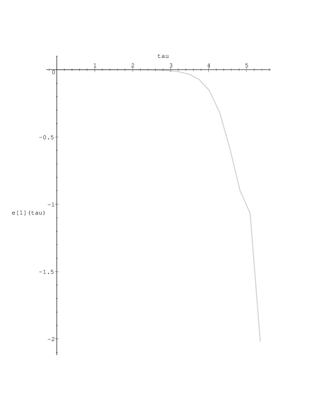
Figure 4: The ${\mathfrak{su}}(3)$ perturbation $\epsilon_{1}(\tau)$ along the unstable manifold. The value $\tau=0$ corresponds to the critical point. Note that $\psi=1+\epsilon_{1}$ monotonically decreases through $0$ and $-1$, from which point it will continue to monotonically decrease.

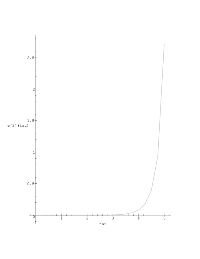
Figure 5: The ${\mathfrak{su}}(3)$ perturbation $\epsilon_{2}$ along the unstable manifold. Note that this is a monotonically increasing function, which is in accordance with the gauge function $\omega_{2}$ having no further zeros.

The analysis of section V has already shown that we have a saddle point here; this notation is convenient merely because the perturbation in $\psi$ decouples from that of $\omega_{2}$ in the linear approximation. From the form of the equation (143), it is clear that $|\psi|$ will be monotonic increasing for $|\psi|>1$. In other words, for $\epsilon_{1}>0$ initially, $\epsilon_{1}>0$ always and $\omega_{1}$ will have no additional zeros for $r>r_{1}$. Hence we need only consider the case where $\epsilon_{1}<0$ initially. Unfortunately the non-linear perturbation equations cannot be integrated analytically and so we present a numerical argument. For initial $\epsilon_{1},\epsilon_{2}$ sufficiently small, the values of $\epsilon_{1}$ and $\epsilon_{2}$ will remain close to those on the unstable manifold for all $\tau<\tau_{1}$ for some $\tau_{1}$, where $\tau_{1}$ can be taken to be as large as we like by making the initial perturbations sufficiently small. Numerical integration of the non-linear equations with the initial point on the unstable manifold and $\epsilon_{1}<0$, shows that $\epsilon_{2}$ increases monotonically and $\epsilon_{1}$ decreases monotonically with just one zero, and cuts through $\epsilon_{1}=-2$ (corresponding to $\psi=-1$), from whence $\psi$ must be monotonically decreasing (see figures 4 and 5). Hence in this case $\omega_{1}$ has ${\bar{n}}_{1}+1$ zeros. $\square$

Lemma VII.8 allows us to prove that every combination of integers $(n_{1},n_{2})$ must correspond to a black hole solution. In the proof of theorem VII.3, we begin with regular solutions with node structure $({\bar{n}}_{2},{\bar{n}}_{2})$ and then from lemma VII.8 there are either regular or singular solutions with node structure $({\bar{n}}_{2}+1,{\bar{n}}_{2})$. Using lemma VII.6, there are then regular solutions having this node structure and the proof of theorem VII.3 follows as before.

So far we have proved the existence of infinitely many ${\mathfrak{su}}(3)$ black holes only for $r_{h}>2$. The remainder of this section will be spent proving the result for $r_{h}\leq 2$. In this case, the points at which the map $f$ is not continuous (which must still exist by the argument used in proving proposition VII.1) do not necessarily correspond to regular black hole solutions: they could also be oscillating solutions. A couple of lemmas concerning oscillating solutions are required before the proofs of proposition VII.1 and theorem VII.3 can be extended.

Lemma VII.9

If $({\bar{\omega}}_{1,h},{\bar{\omega}}_{2,h})$ leads to an oscillating solution with $\omega_{1}(\tau)\rightarrow 0$ and $\omega_{2}(\tau)\rightarrow 1$ as $\tau\rightarrow\infty$, and $\omega_{2}$ has ${\bar{n}}_{2}$ zeros, then all $(\omega_{1,h},\omega_{2,h})$ sufficiently close to $({\bar{\omega}}_{1,h},{\bar{\omega}}_{2,h})$ lead to one of the following types of solution:

1. an oscillating solution in which $\omega_{1}(\tau)\rightarrow 0$ and $\omega_{2}(\tau)\rightarrow 1$ as $\tau\rightarrow\infty$, with $\omega_{2}$ having at least ${\bar{n}}_{2}$ zeros;

2. given $n_{0}$, either a regular or a singular solution with $n_{1}\geq n_{0}$ and $n_{2}\geq{\bar{n}}_{2}$.

3. an $S_{\infty}$ solution.

Proof
Since in the original solution $\omega_{1}$ has infinitely many zeros and the solutions are analytic in $\tau$ and the starting values, there is some $\tau_{1}$ such that all solutions with $(\omega_{1,h},\omega_{2,h})$ sufficiently close to $({\bar{\omega}}_{1,h},{\bar{\omega}}_{2,h})$ must have at least $n_{0}$ zeros of $\omega_{1}$ and ${\bar{n}}_{2}$ zeros of $\omega_{2}$ for $\tau<\tau_{1}$, and all variables will be close to their asymptotic values. $\square$

Lemma VII.10

There exists $({\bar{\omega}}_{1,h},{\bar{\omega}}_{2,h})\in D$ corresponding to an oscillating solution.

Proof
From [7], we know that there are points on the line $\omega_{1,h}=\omega_{2,h}$ corresponding to $S_{\infty}$ solutions. By continuity, there is a neighbourhood $D_{0}$ of the line $\omega_{1,h}=\omega_{2,h}$ corresponding to $S_{\infty}$ solutions. However, lemma VII.5 still applies in this case, so that the regular solutions on the line $\omega_{1,h}=\omega_{2,h}$ will have singular solutions in $D$ sufficiently close to them for which $r(\tau_{0})>2$. Therefore, by lemma VII.9, there must be points in $D$ which correspond to oscillating solutions. $\square$

The proofs of proposition VII.1 and theorem VII.3 are now exactly the same as for $r_{h}>2$. Since oscillating solutions have an infinite number of zeros for at least one of the gauge field functions, and using lemma VII.9, regular solutions are still needed to separate singular solutions having different node structures.

VIII ${\mathfrak{su}}(N)$ black holes

The detailed discussion of the previous section now enables us to proceed quite swiftly to the analogues of proposition VII.1 and theorem VII.3 for general $N$. The method of proof will be by induction, which was the basic idea used in the previous section, where we proved existence for ${\mathfrak{su}}(3)$ exploiting known results about ${\mathfrak{su}}(2)$.

The first step is to illustrate how solutions which are from ${\mathfrak{su}}(n)$, where $n<N$ may be embedded in the ${\mathfrak{su}}(N)$ framework. Firstly, exactly as in the $N=3$ case, we may embed neutral ${\mathfrak{su}}(2)$ solutions [11]. We set $\omega_{j}(r)={\sqrt{j(N-j)}}\omega(r)$ and introduce a scaled variable $R=\lambda_{N}r$, where

$$\lambda_{N}=\left(\frac{1}{6}N(N+1)(N-1)\right)^{\frac{1}{2}}.$$ (147)

Then the field equations are exactly the same as the ${\mathfrak{su}}(2)$ ones, and the existence of solutions follows directly [11]. Secondly, charged, effectively ${\mathfrak{su}}(N-1)$ solutions can be generated by setting $\omega_{1}\equiv 0$ (or $\omega_{N-1}\equiv 0$) [4]. Although the equation for $m^{\prime}$ in this situation is not the same as for neutral ${\mathfrak{su}}(N-1)$ black holes, due to the charge, the regular equations discussed in section II are unchanged, so the proof of existence of neutral ${\mathfrak{su}}(N-1)$ black holes extends naturally to this case.

For $N>3$, there are additional embeddings which arise from setting at least one of $\omega_{2},\ldots,\omega_{N-2}\equiv 0$, so that the gauge field equations decouple into two or more sets of coupled components, the sets being coupled to each other only through the metric. Solutions of this form have been found numerically in [4]. We illustrate how the existence of black holes of this type may be proved by considering the simplest case, which arises when $N=4$. In this case, we have three non-zero gauge field functions, $\omega_{1},\omega_{2},\omega_{3}$. If we set $\omega_{2}\equiv 0$, then the field equations take the form

$$r^{2}\mu\omega_{1}^{\prime\prime} = -\left(2m-2r^{3}p_{\theta}\right)\omega_{1}^{\prime}-\left(1-\omega_{1}^{2}\right)\omega_{1}$$ (148)

$$r^{2}\mu\omega_{3}^{\prime\prime} = -\left(2m-2r^{3}p_{\theta}\right)\omega_{3}^{\prime}-\left(1-\omega_{3}^{2}\right)\omega_{3}$$ (149)

$$m^{\prime} = \left(\mu G+r^{2}p_{\theta}\right)$$ (150)

$$\frac{S^{\prime}}{S} = \frac{2G}{r}$$ (151)

where

$$G=\omega_{1}^{{}^{\prime}2}+\omega_{3}^{{}^{\prime}2},\qquad p_{\theta}=\frac{1}{2r^{4}}\left(\left[\omega_{1}^{2}-1\right]^{2}+\left[\omega_{3}^{2}-1\right]^{2}+8\right).$$ (152)

These equations look very much like two uncoupled ${\mathfrak{su}}(2)$ degrees of freedom, however, the two $\omega$’s are (albeit weakly) coupled. The fact that we have two gauge field functions here means that we can use the methods of section VII to prove the existence of regular black hole solutions. In fact, all the results of that section carry directly over to this situation on replacing $\omega_{2}$ there by $\omega_{3}$ here. There is one exception. The equations (148,149) are slightly different from those in section VII and this enables us to strengthen lemma VII.5.

Lemma VIII.1

If $({\bar{\omega}}_{1,h},{\bar{\omega}}_{3,h})$ leads to a regular black hole solution with $\omega_{1}$ having ${\bar{n}}_{1}$ nodes and $\omega_{3}$ having ${\bar{n}}_{3}$ nodes, then all $(\omega_{1,h},\omega_{3,h})$ sufficiently close to $({\bar{\omega}}_{1,h},{\bar{\omega}}_{3,h})$ lead to regular or singular solutions with $\omega_{1}$ having either ${\bar{n}}_{1}$ or ${\bar{n}}_{1}+1$ zeros and $\omega_{3}$ having either ${\bar{n}}_{3}$ or ${\bar{n}}_{3}+1$ zeros.

Proof
Since the solutions are continuous in the starting parameters and $r$, for $(\omega_{1,h},\omega_{3,h})$ sufficiently close to $({\bar{\omega}}_{1,h},{\bar{\omega}}_{3,h})$, there is some $r_{1}$ such that $\omega_{1}$ will have ${\bar{n}}_{1}$ zeros and $\omega_{3}$ will have ${\bar{n}}_{3}$ zeros for $r<r_{1}$. There will also be an $r_{2}>r_{1}$ such that all field variables are close to their asymptotic values for $r\in[r_{1},r_{2}]$. The flat space field equations (see section V) decouple completely since $\omega_{2}\equiv 0$, and so the phase plane analysis of [7] is valid in this case. The phase plane analysis enables us to be more precise about the number of zeros of the perturbed gauge field functions, unlike the more general case where the phase space had more than two coupled dimensions. Therefore the conclusions of [7, proposition 22] can be applied directly here and each gauge field function can have at most one zero for $r>r_{2}$. $\square$

With this more powerful lemma, the analysis of section VII reaches the conclusion that there are regular black hole solutions of the required form for each $r_{h}$ and node structure $(n_{1},n_{3})$.

For general $N$, similar embeddings of the form of two or more ${\mathfrak{su}}(n)$ ($n<N$) type solutions separated by at least one $\omega_{j}\equiv 0$ are possible, and the existence proof follows the lines outlined above for ${\mathfrak{su}}(4)$, using the existence of solutions for the various ${\mathfrak{su}}(n)$. The allowed node structures will be exactly the same as those for the constituent ${\mathfrak{su}}(n)$ components. We refer the reader to [4] for further details of the construction of solutions of this form.

The remainder of this section will be spent outlining briefly the proof of the following theorem. By ‘types’ in the statement of the theorem we mean the node structures of the gauge field functions.

Theorem VIII.2

There exist infinitely many types of regular black hole solutions of the ${\mathfrak{su}}(N)$ Einstein-Yang-Mills equations including genuine ${\mathfrak{su}}(N)$ solutions and embedded solutions.

All that remains to prove this theorem is to show the existence of genuine ${\mathfrak{su}}(N)$ solutions in which the node structures of the gauge field functions are not all the same. We assume for an inductive hypothesis that the theorem holds for all $n<N$. The situation is slightly complicated by the fact that our parameter space consisting of the $\omega_{j,h}$’s is now $N-1$-dimensional. We consider the $\omega_{1,h}=0$ hyperplane, on which we know the solution space by the inductive hypothesis. The map $f$ (see section VII) now takes ${\mathbb{R}}^{N-1}$ to ${\mathbb{B}}^{N-1}\times[0,1]$. Again, we need only consider the action of $f$ on those parts of ${\mathbb{R}}^{N-1}$ in which no $\omega_{j,h}$ vanishes. We restrict attention to one of the disjoint spaces so generated without loss of generality. Lemma VII.2 and the proof of the ${\mathfrak{su}}(N)$ equivalent of proposition VII.1 now carry over to prove the existence of genuine ${\mathfrak{su}}(N)$ black holes. Lemmas VII.4, VII.6 and VII.7 now hold for a point $(0,{\bar{\omega}}_{2,h},\ldots,{\bar{\omega}}_{N-1,h})$ corresponding to a charged solution, and lemmas VII.5 and VII.9 carry straight over to a point $({\bar{\omega}}_{1,h},{\bar{\omega}}_{2,h},\ldots,{\bar{\omega}}_{N-1,h})$ which leads to a regular black hole solution or oscillating solution respectively. These are the ingredients necessary for the simple argument which leads to the proof of theorem VII.3 and hence theorem VIII.2 for both $r_{h}^{2}>\frac{1}{6}N(N+1)(N-1)$ (in which case no oscillating solutions exist), and $r_{h}^{2}\leq\frac{1}{6}N(N+1)(N-1)$. Note that, as in the ${\mathfrak{su}}(3)$ case, we are not able to prove analytically that every sequence of integers $(n_{1},n_{2},\ldots,n_{N-1})$ corresponds to a black hole solution whose gauge functions have this node structure, although it might reasonably be expected that this is indeed the case.

IX Results and conclusions

In this paper we have proved the existence of a vast number of hairy black holes in ${\mathfrak{su}}(N)$ Einstein-Yang-Mills theories. The solutions are described by N-1 parameters, corresponding to the number of nodes of the gauge field functions. The result of [12] tells us that each of these solutions will have a topological instability, similar to the flat-space “sphaleron”, as was the case for ${\mathfrak{su}}(2)$ black holes. This instability does not necessarily diminish the physical importance of these objects, as they may have an important role in processes such as cosmological particle creation [15].

We now briefly mention another important reason for studying ${\mathfrak{su}}(N)$ black holes, namely the behaviour of the solutions as $N\rightarrow\infty$. Black holes in ${\mathfrak{su}}(\infty)$ Einstein-Yang-Mills theory would possess an infinite amount of hair, requiring an infinite number of parameters to describe their geometry. This might be analogous to the “W-hair” found in non-critical string theory [16], and have drastic consequences for the Hawking radiation, information loss and quantum decoherence processes associated with black holes. The existence of infinite amounts of hair might also render such objects stable. It is already known that the ${\mathfrak{su}}(\infty)$ Lie algebra is simply that of the diffeomorphisms of the sphere [17]. This means that the limit as $N\rightarrow\infty$ cannot be taken smoothly, in particular the results of the present paper are only valid when $N$ is finite. We hope to return to this matter in a subsequent publication.

Figure 1: The $(\omega_{1,h},\omega_{2,h})$ plane, with a schematic representation of the lines representing regular black hole solutions, which are also denoted by crosses.

Figure 2: Schematic representation of the set ${\mathbb{B}}\times[0,1]$, corresponding to the space of parameters of the ${\mathfrak{su}}(3)$ solutions in section VII. The horizontal axis represents $N_{1}$, the number of nodes of the gauge function $\omega_{1}$, and the vertical axis $R_{m}$, which characterizes the maximum value of the radial co-ordinate $r$ for each solution.

Figure 3: The projection of the parameter space of solutions on to the set ${\mathbb{B}}\times{\mathbb{B}}$. The axes are $N_{1}$ and $N_{2}$, the number of nodes of the respective gauge functions $\omega_{1}$ and $\omega_{2}$. The crosses indicate schematically the points in this set.

References

• [1] R. Bartnik and J. McKinnon, Phys. Rev. Lett. 61, 141 (1988)
• [2] P. Bizon, Phys. Rev. Lett. 64, 2844 (1990)
• [3] B. R. Greene, S. D. Mathur and C. M. O’Neill, Phys. Rev. D47, 2242 (1993)
P. Kanti, N. E. Mavromatos, J. Rizos, K. Tamvakis and E. Winstanley, Phys. Rev. D54, 5049 (1996)
T. Torii, K-I Maeda and T. Tachizawa, Phys. Rev. D52, 4272 (1995)
S. Droz, M. Heusler and N. Straumann, Phys. Lett. B268, 371 (1991)
G. Lavrelashvili and D. Maison, Nucl. Phys. B410, 407 (1993)
• [4] B. Kleihaus, J. Kunz and A. Sood, Preprint hep-th/9705179
• [5] B. Kleihaus, J. Kunz and A. Sood, Phys. Lett. 354B, 240 (1995)
• [6] N. E. Mavromatos and E. Winstanley, Phys. Rev. D53, 3190 (1996)
• [7] P. Breitenlohner, P. Forgács and D. Maison, Comm. Math. Phys. 163, 141 (1994)
• [8] J. A. Smoller and A. G. Wasserman, J. Math. Phys. 36, 4301 (1995)
• [9] J. Smoller, A. Wasserman and S.-T. Yau, Comm. Math. Phys. 154, 377 (1993)
• [10] H. P. Künzle, Class. Quant. Grav. 8, 2283 (1991)
• [11] H. P. Künzle, Comm. Math. Phys. 162, 371 (1994)
• [12] O. Brodbeck and N. Straumann, Zürich University Preprint, ZU-TH 38/94, gr-qc/9411058.
• [13] E. A. Coddington and N. Levinson, “The Theory of Ordinary Differential Equations”, McGraw-Hill, New York (1955)
• [14] A. A. Ershov and D. V. Gal’tsov, Phys. Lett. 150A, 159 (1990)
• [15] G. W. Gibbons and A. R. Steif, Phys. Lett. B320, 245 (1994)
• [16] See, for example, J. Ellis, N. E. Mavromatos and D. V. Nanopoulos, “A non-critical string approach to black holes, time and quantum dynamics”, Lectures presented at the International School of Sub-Nuclear Physics, Erice, published in the proceedings, Sub-Nuclear Series 31, 1 (1994) (World Scientific)
• [17] E. G. Floratos, J. Iliopoulos and G. Tiktopoulos, Phys. Lett. B217, 285 (1989)
$\omega_{2,h}$ $\omega_{1,h}$ $\omega_{1,h}=\omega_{2,h}$ $\times$ $\times$ $\times$ $\times$ $\times$ $\times$ $\times$ $\times$ $\times$