New Orthogonal Body–Fitting Coordinates for Colliding Black Hole Spacetimes

Abstract

We describe a grid generation procedure designed to construct new classes of orthogonal coordinate systems for binary black hole spacetimes. The computed coordinates offer an alternative approach to current methods, in addition to providing a framework for potentially more stable and accurate evolutions of colliding black holes. As a particular example, we apply our procedure to generate appropriate numerical grids to evolve Misner’s axisymmetric initial data set representing two equal mass black holes colliding head–on. These new results are compared with previously published calculations, and we find generally good agreement in both the waveform profiles and total radiated energies over the allowable range of separation parameters. Furthermore, because no specialized treatment of the coordinate singularities is required, these new grids are more easily extendible to unequal mass and spinning black hole collisions.

I Introduction

After the first attempt in 1964 by Hahn and Lindquist [1] to solve the problem of colliding black holes, a long–term and relatively successful program was initiated in the late 1960s by DeWitt et. al. (see DeWitt, Čadež, Smarr, and Eppley [2, 3, 4, 5], which we henceforth collectively refer to as DCSE). Their efforts were concentrated on simulating the axisymmetric head–on collision of two equal mass black holes using the time symmetric Misner data [6] for initial conditions. This data set possesses the “double Einstein–Rosen bridge” [7] topology in which two asymptotically flat sheets are joined by two throats representing non-rotating black holes. The throats are two–spheres that are invariant under an isometry operation identifying both sheets and, from a numerical standpoint, serve as a boundary across which a particular form of Neumann boundary condition must be imposed on the evolved quantities to preserve the isometry.

DCSE developed the 2D Čadež [2] coordinate system to numerically integrate and evolve the axisymmetric Einstein equations. The Čadež coordinates are curvilinear body–fitting coordinates that conform to the two black hole throats and become spherical at asymptotic infinity. The advantages of this coordinate system (and any other appropriate body–fitting system) include: (1) simplified boundary conditions at the black hole throats, (2) natural spherical–like grids which mimic the background Schwarzschild geometry that the solutions approach at late times, (3) simplification of waveform extraction calculations in the wave zone, and (4) exponential stretching of the grid in the radial direction which covers enough of the spacetime that asymptotic flatness can be applied to the conformal metric components at the outer grid edges. However, these conveniences are offset somewhat by the singular saddle point introduced by the coordinate transformation at the origin midway between the two black holes. DCSE attempted to deal with the saddle point by evolving the cylindrical (not Čadež) metric components everywhere on the Čadež grid and performing discretizations using chain rule derivatives. Also, because black hole spacetimes can generate pathologically steep delta–function–like peaks in the metric components (assuming singularity avoiding time slices), numerical evolutions can quickly become unstable even if the inherent symmetries are exploited in choosing the appropriate numerical grid and the evolved variables. Additionally, it is well known [3, 4] that an axis instability can be triggered in numerical evolutions of axisymmetric spacetimes. For all of these reasons, the computations of DCSE remained uncertain with error bars of order 100% [8].

Recently, Anninos, Hobill, Seidel, Smarr and Suen [9, 10, 11] (henceforth referred to as Papers I, II and III respectively) improved upon the DCSE calculations by introducing a shift vector to diagonalize the Čadež metric and to evolve these components on the Čadež grid, thus suppressing the axis instability which is especially sensitive to the off–diagonal elements. The problem with the coordinate singularity at the origin was treated by constructing a cylindrical coordinate “patch” to cover regions near the saddle point. The results of Anninos et al. are accurate to a few percent in the dominant wave signal for black holes which are initially placed at close to moderate separation distances. For larger initial separations (greater than about $10M$, where $M$ is the single black hole mass), the evolutions become increasingly more inaccurate due in part to the fact that the saddle point remains within the causally connected regions of spacetime for longer periods of time as the black holes take longer to collide at the origin. If the black holes are initially separated by even greater distances (more than about $20M$), the evolutions become unstable and break down altogether.

In short, the goal of long–term stable and accurate computations of highly separated colliding black holes has yet to be achieved. Here we propose two new classes of orthogonal body–fitting coordinate systems that are well–suited to the axisymmetric geometry of two colliding black holes, and that appear promising to improve upon current calculations. The new coordinates remove the singular saddle point from its obtrusive position at the origin and thus offer a potentially cleaner and more stable method of solution. Because we require spherical coordinate lines at the throats and in the far field, singular points are unavoidable. However, the saddle point singularities can be relocated along the $z$–axis to either the south or north pole of the top hole (and thus the north or south pole of the bottom hole, respectively), assuming the two holes are aligned vertically along the $z$–axis. We refer to the former system where the singularities face the opposite black hole as the class I system: class II refers to the latter case with the singularities facing away from the opposing throats.

We are thus able to construct two new classes of coordinate systems, replacing the single singularity at the origin with a pair of saddle singularities on the throats. An advantage of transplanting the coordinate singularities to the throats prevents the black holes from “crashing” into a saddle point during the numerical evolutions. Instead, we implement a singularity avoiding lapse function that is zero on the throat, so that the evolution along the throat freezes in time. In addition, the (maximal) time slicing used in the evolutions will rapidly absorb coordinate lines into the event horizon and the saddle points will fall further inside the causally disconnected portion of the evolved spacetime where the lapse collapses exponentially to zero, providing an additional stabilizing element.

The following sections describe our hybrid analytic/numerical procedure to generate discrete grids for axisymmetric binary black hole systems. Sec. II introduces grid generating techniques in general and describes the particular analytic prescriptions that we developed for specifying one of the coordinates. Sec. III describes the numerical calculation of the second coordinate orthogonal to the first, as well as the techniques used to compute the Jacobian matrix required for the coordinate transformations, and the tests which can be used to monitor the accuracy in which the coordinate systems and Jacobians are constructed. Results from actual numerical evolutions are presented in Sec. IV and compared with previously published calculations. We summarize our results in Sec. V.

II Generating Body–fitting coordinates: The Specified Coordinate

A general and common method of constructing body–fitting coordinates is to let the curvilinear coordinates ($\eta$, $\xi$) satisfy the following elliptic partial differential equations [12]

$$\partial_{xx}\xi+\partial_{yy}\xi = P(\eta,~{}\xi)~{},$$ (2)

$$\partial_{xx}\eta+\partial_{yy}\eta = Q(\eta,~{}\xi)~{},$$ (3)

where $P(\xi,\eta)$ and $Q(\xi,\eta)$ are generating functions that can be used to adjust the behavior of the curvilinear coordinates in the physical domain. Because the boundaries are typically irregular in Cartesian coordinates (or cylindrical coordinates in our black hole work), and the ($\eta$, $\xi$) coordinates are uniform in the transformed plane, it is desirable to carry out the computations in the transformed plane, switching the dependent and independent variables. Equations (II) can be inverted to yield

$$\alpha\partial_{\xi\xi}x-2\beta\partial_{\eta\xi}x+\gamma\partial_{\eta\eta}x+J^{2}\left(P\partial_{\xi}x+Q\partial_{\eta}x\right) = 0~{},$$ (5)

$$\alpha\partial_{\xi\xi}y-2\beta\partial_{\eta\xi}y+\gamma\partial_{\eta\eta}y+J^{2}\left(P\partial_{\xi}y+Q\partial_{\eta}y\right) = 0~{},$$ (6)

where $\alpha=\partial_{\eta}x^{2}+\partial_{\eta}y^{2}$, $\beta=\partial_{\xi}x\partial_{\eta}x+\partial_{\eta}y\partial_{\xi}y$, $\gamma=\partial_{\xi}x^{2}+\partial_{\xi}y^{2}$, and $J=\partial_{\xi}x\partial_{\eta}y-\partial_{\eta}x\partial_{\xi}y$. The problem of grid generation then reduces to solving a coupled set of nonlinear elliptic partial differential equations subject to the appropriate boundary conditions, which can themselves be intrinsically coupled in a complicated manner. Although the elliptic solution approach is a general and straight–forward one, other methods such as conformal mapping, algebraic transformations, and hyperbolic solutions of partial differential equations have also been developed (see [12] for a review of grid generation techniques).

In this paper, we present an altogether different and much simplified procedure that does not require one to solve coupled nonlinear elliptic equations. The idea rests on the notion that the grid generation process is greatly simplified if one of the coordinates can be specified analytically. Taking this coordinate as the one aligned asymptotically with either the radial or the angular direction, we show in this section how to construct a natural “specified” coordinate for three different classes of grids as characterized by the location of the singularity: class I (II) with two singular saddle points, one on each of the throats on the axis closest to (furthest from) the origin; and class III which are Čadež–like coordinates with a single singular point at the origin $\rho=z=0$. We note that the function one chooses for the specified coordinate must solve the necessary boundary conditions, but is not restricted to satisfy any particular elliptic equation.

Before we continue, a few notational comments are in order. Four axisymmetric coordinate systems are utilized in this paper: the combination $(\rho,z)$ refers to standard cylindrical coordinates, ($r$, $\theta$) denotes standard polar coordinates, ($\zeta$, $\xi$) are the radial– and angular–like body fitting coordinates, and ($\eta$, $\xi$) represent the logarithmic radial– and angular–like body fitting coordinates (note the two $\xi$ coordinates are identical). Finally we characterize the location of the two black holes by their radius $a_{1}$ ($a_{2}$) and vertical distance from the origin along the $z$–axis $z_{1}$ ($z_{2}$), where $z_{1}$ ($z_{2}$) represents the absolute distance of the throat center from the origin, and the upper (lower) black hole is denoted by the subscript 1 (2).

A The Class I System

The class I coordinate system has a coordinate (saddle–type) singularity where each of the throats meet the axis closest to the origin (see Fig. II A). A singularity is generated at these points by requiring that a radial–like coordinate $\zeta$ be zero on both of the throats and the entire section of the axis connecting the throats. Lines of constant $\zeta$ will then transform from “peanut”–like surfaces near the throats to radial circles at infinity. The two throats and the axis between the throats in this case make up the line $\eta=0$. The axis above (below) the top (bottom) hole is the angular coordinate value $\xi=0$ ($\pi$). In the equal mass case, the equator is the line $\xi=\theta=\pi/2$. The boundary conditions are shown in Fig. II A and Fig. II A in the ($\rho,z$) and ($\zeta,\xi$) planes respectively.

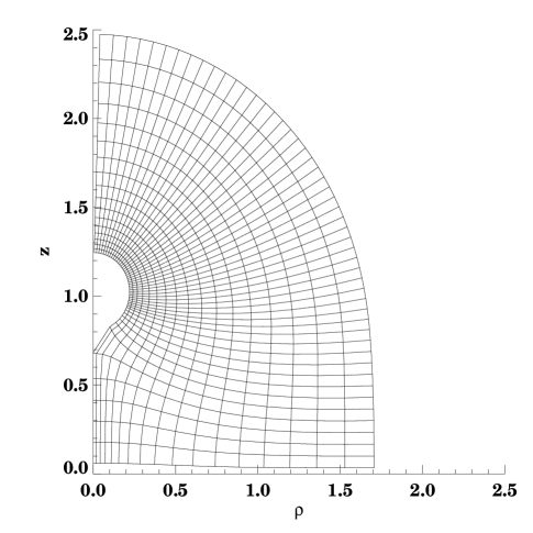
FIG. 1.: Class I coordinates for the $\mu=2.2$ Misner data.
 

An exponentially stretched radial coordinate satisfying the appropriate boundary conditions can be generated by first defining two radial distances from the two throats

$$d_{1} = \sqrt{\rho^{2}+(z-z_{1})^{2}}-a_{1},$$ (7)

$$d_{2} = \sqrt{\rho^{2}+(z+z_{2})^{2}}-a_{2},$$ (8)

and a third distance measure

$$d_{3} = \frac{1}{2}\left[\sqrt{\rho^{2}+(z-z_{1}+a_{1})^{2}}+\right.$$ (10)

$$\left.\sqrt{\rho^{2}+(z+z_{2}-a_{2})^{2}}-(z_{1}+z_{2}-a_{1}-a_{2})\right],$$

defining an “elliptic” radial coordinate that is zero on the segment along the $z$–axis extending from $z=z_{1}$ to $z=-z_{2}$. (We note that the square root radicals implicitly refer to the absolute or positive root.) The actual curvilinear “radial” coordinates, $\zeta$ and $\eta$, are then constructed from these distance components by

$$\zeta=\frac{(2\kappa_{1}+1)d_{1}d_{2}d_{3}}{d_{1}d_{2}+\kappa_{1}(d_{1}d_{3}+d_{2}d_{3})},$$ (11)

and

$$\eta=\sinh^{-1}\left(\frac{\zeta}{\kappa_{2}}\right).$$ (12)

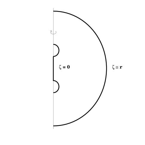
FIG. 2.: The “radial” ($\zeta$) boundary conditions for the class I coordinate system.
 

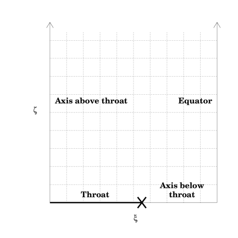
FIG. 3.: The class I schematic mapping of the rectangular $(\zeta,\xi)$ domain in relation to the throat, axis, and equator. The cross indicates the location of the coordinate singularity at the intersection of the throat and axis closest to the equator.
 

Both are zero on the “spectacle” boundary of Fig. II A by construction. Equations (11) and (12) also have the proper behavior in the asymptotic limit where both $\rho$ and $z$ tend to infinity, ie., $\zeta\rightarrow r$ and $\eta\rightarrow\log(r/\kappa_{2})$. The parameters $\kappa_{1}$ and $\kappa_{2}$ are introduced so the coordinate systems can be “tuned” to improve the stability of evolutions. In particular, $\kappa_{1}$ controls the relative importance between the “elliptic” radius ($d_{3}$) and the two distance–from–throat radii ($d_{1}$ and $d_{2}$), and affects the shape of the grid close to the axis between the holes. By adjusting $\kappa_{1}$, the grid can be pushed away from or drawn closer to the axis in this region, effectively increasing or decreasing the resolution between the holes in the $\rho$ direction. $\kappa_{2}$ controls the asymptotic behavior of the coordinates in the far zone. Typical values for evolutions depend on the geometry of the system, and range from ($\kappa_{1}$, $\kappa_{2}$) = (1, 2) for the $\mu=1.2$ case, to (0.7, 2) for the $\mu=2.7$ case, where $\mu$ is the Misner parameter defined in Sec. IV A.

B The Class II System

The class II coordinate system has a saddle point where each of the throats meet the axis furthest from the origin (see Fig. II B). A singularity is generated at these points by requiring that an angular–like coordinate $\xi$ be zero ($\pi$) along the throat of the top (bottom) black hole and along the axis above (below) the top (bottom) throat. The coordinate $\xi$ also asymptotes to the polar angular coordinate $\theta$. The north (south) throat in this case is a line of constant $\xi=0$ ($\pi$) between $\zeta=0$ and some finite $\zeta$ value. The axis above (below) the north (south) throat is on the same constant $\xi$ line as the corresponding throats. The axis between the two throats is the line $\zeta=0$. In the equal mass case, the equator is the line $\xi=\pi/2$. The boundary conditions and mapping are shown in Fig. II B and Fig. II B in the ($\rho$, $z$) and ($\zeta$, $\xi$) planes respectively.

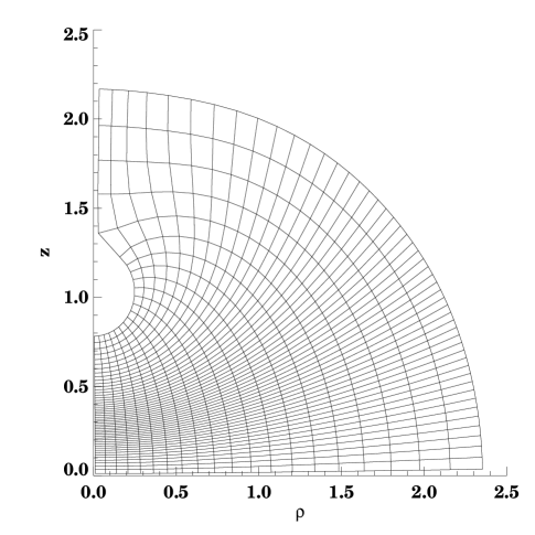
FIG. 4.: Class II coordinates for the $\mu=2.2$ Misner data.
 

FIG. 5.: The “angular” ($\xi$) boundary conditions for the class II coordinates.
 

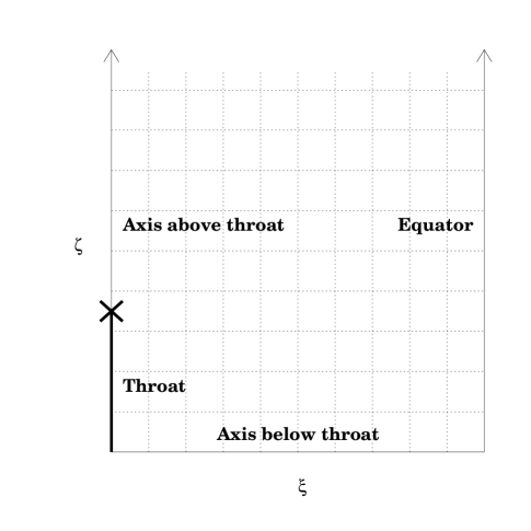
FIG. 6.: The class II schematic mapping of the rectangular $(\zeta,\xi)$ domain in relation to the throat, axis, and equator. The cross indicates the location of the coordinate singularity at the intersection of the throat and axis furthest from the equator.
 

The class II system can be generated by first defining two radial distances similar to the class I case

$$d_{1a} = \rho^{2}+(z-z_{1})^{2}-a_{1}^{2},$$ (13)

$$d_{2a} = \rho^{2}+(z+z_{2})^{2}-a_{2}^{2},$$ (14)

and two “hyperbolic” radial coordinates

$$d_{1b} = -\sqrt{\rho^{2}+(z+z_{2}+a_{2})^{2}}$$ (15)

$$+ \sqrt{\rho^{2}+(z-z_{1}-a_{1})^{2}}+(z_{1}+z_{2}+a_{1}+a_{2}),$$ (16)

$$d_{2b} = +\sqrt{\rho^{2}+(z+z_{2}+a_{2})^{2}}$$ (17)

$$- \sqrt{\rho^{2}+(z-z_{1}-a_{1})^{2}}+(z_{1}+z_{2}+a_{1}+a_{2}),$$ (18)

which go to zero along the axis above and below the holes respectively. These coordinates can be combined to construct a function that is zero on the top hole’s throat and along the axis above it ($d_{1}$), and a function that is zero on the bottom hole’s throat and along the axis below it ($d_{2}$)

$$d_{1} = \frac{d_{1a}d_{1b}}{\rho^{2}+(z-z_{1})^{2}},$$ (19)

$$d_{2} = \frac{d_{2a}d_{2b}}{\rho^{2}+(z+z_{2})^{2}}.$$ (20)

The two functions $d_{1}$ and $d_{2}$ are in turn combined to create a common function $f$ that approaches $+\infty$ as $d_{1}\rightarrow 0$, and $-\infty$ as $d_{2}\rightarrow 0$

$$f=(a_{1}+a_{2}+z_{1}+z_{2})\left(\frac{1}{d_{1}}-\frac{1}{d_{2}}\right).$$ (21)

Finally, the function $f$ is converted to an angular–like coordinate by

$$\xi={\rm ArcCot}\left(\frac{{\rm sign}(f)}{\sqrt{2}}\sqrt{-1+\sqrt{1+f^{2}}}\right).$$ (22)

The angular coordinate in Eqn. (22) has the desired properties of being zero on the throat of the top hole and along the axis above it, $\pi$ on the bottom hole and along the axis below it, and approaches the normal spherical coordinate $\theta$ in the asymptotic limit $r\rightarrow\infty$.

In the class I system, the value of the second coordinate $\xi$ is specified on the outer grid edge to be the angular polar coordinate $\theta$. There is slightly more freedom in class II for specifying the second coordinate $\eta$ at small $r$, since we only require that $r=e^{\eta}$ near the outer edge of the grid. We therefore define

$$r=2\sinh\eta+k_{1}\eta$$ (23)

to be the radial coordinate. Because the throat is described by the first several $\eta$ zones (see Fig. II B), $k_{1}$ effectively controls the resolution along and near the throat boundary.

C The Class III System: Čadež–like Coordinates

Čadež coordinates (see Fig. II C) are related to cylindrical coordinates through the following semi–analytic complex transformation

$$\eta + i\xi=\frac{1}{2}\left[\ln\left(z+z_{0}+i\rho\right)+\ln\left(z-z_{0}+i\rho\right)\right]$$ (25)

$$+\sum_{n=1}^{\infty}C_{n}\left[\frac{1}{(z+z_{0}+i\rho)^{n}}+\frac{1}{(z_{0}-z-i\rho)^{n}}\right]~{},$$

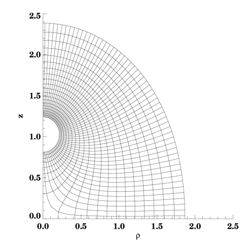
where $z=\pm z_{0}$ are the locations of the throat centers. The constant radial and angular lines lie along the field and equipotential lines of two equally charged metallic cylinders located at the centers of the two throats. Hence the lines of constant $\eta$ are spherical along the throats and in the asymptotic far field, and a singular saddle point is introduced midway between the two black holes at the origin $\rho=z=0$. The coefficients $C_{n}$ are determined numerically by a least squares procedure to set the throats (defined by $\rho_{th}^{2}+(z_{th}\pm z_{0})^{2}=a^{2}$, where $a=a_{1}=a_{2}$ is the throat radius) to lie on an $\eta=\eta_{0}=$ constant coordinate line. FIG. 7.: Čadež coordinates for the Misner data with separation parameter $\mu=2.2$.
 

It is relatively easy to generate a Čadež–like system using our grid generation prescription. A radial coordinate is required which vanishes on the throats (and only on the throats) and asymptotes to $r$ as $\rho$ and $z$ tend to infinity. Clearly, this can be satisfied with

$$\zeta=\frac{d_{1}d_{2}}{d_{1}+d_{2}}\left(1-k_{1}\exp\left(-k_{2}\rho^{2}-k_{3}z^{2}\right)\right),$$ (26)

where

$$d_{1} = \sqrt{\rho^{2}+(z-z_{1})^{2}}-a_{1},$$ (27)

$$d_{2} = \sqrt{\rho^{2}+(z+z_{2})^{2}}-a_{2},$$ (28)

and the parameters $k_{1}$, $k_{2}$ and $k_{3}$ are introduced to control the behavior and resolution of the coordinates near the saddle point at the origin. In contrast with the Čadež coordinates, we note that the Cauchy-Riemann relations are not satisfied for this coordinate system.

III Generating the Second Coordinate and Other Numerical Issues

We have developed two different methods for computing the second (unspecified) coordinate and to establish the positions of the $(\eta,\xi)$ grid points in the cylindrical coordinate $(\rho,z)$ space. In addition to evaluating the grid node positions, it is also necessary to compute the Jacobian matrix elements (ie., the coordinate derivatives) accurately. The Jacobian matrix and its inverse are needed to transform metric functions between the ($\rho$, $z$) and ($\eta$, $\xi$) spaces and to perform chain rule differentiations of the cylindrical metric functions on the curvilinear grids in the coordinate “patch” regions described in Sec. IV. We turn first to the computation of the Jacobian, and then to the generation of the second coordinate.

A Computing the Jacobian

In order to effectively use the curvilinear grids in numerical evolutions, it is important to generate the Jacobian matrix and its inverse as accurately as possible, since the gravitational waves emitted from the collisions are expected to be very weak in relation to the background geometry. Knowing the matrix components amounts to knowing, at each point on the grids, the coordinate derivatives $\partial\rho/\partial\eta$, $\partial\rho/\partial\xi$, $\partial z/\partial\eta$ and $\partial z/\partial\xi$. A naive approach would be to simply evaluate these derivatives numerically at each point, after the grid has been calculated, using a second or higher order discretization stencil. Instead, we adopt a more accurate procedure and take advantage of the fact that the derivatives of the specified coordinate are known analytically. In this way, only two of the elements need to be computed numerically.

The Jacobian matrix and its inverse can be written as

$$\left[\begin{array}[]{cc}\partial_{\eta}\rho&\partial_{\eta}z\\ \partial_{\xi}\rho&\partial_{\xi}z\end{array}\right]=\frac{1}{J}\left[\begin{array}[]{cc}\partial_{z}\xi&-\partial_{\rho}\xi\\ -\partial_{z}\eta&\partial_{\rho}\eta\end{array}\right],$$ (29)

where $J=\partial_{\rho}\eta\,\partial_{z}\xi-\partial_{z}\eta\,\partial_{\rho}\xi$ is the Jacobian determinant. One can show from the orthogonality of the $(\rho,z)$ and $(\eta,\xi)$ coordinates that the first derivatives obey the Cauchy–Riemann–like conditions

$$\partial_{z}\eta = \sigma\partial_{\rho}\xi,$$ (31)

$$\partial_{\rho}\eta = -\sigma\partial_{z}\xi,$$ (32)

where $\sigma=\sqrt{g_{\xi\xi}/g_{\eta\eta}}$, and $g_{ij}$ is the metric in curvilinear coordinates. In the class I case, two components of the inverse Jacobian, $\partial_{\rho}\eta$ and $\partial_{z}\eta$, are known analytically. Thus, using the relationships (29) and (29), the following class I elements are determined exactly from the analytic expressions

$$\partial_{\eta}z = \frac{\partial_{z}\eta}{(\partial_{\rho}\eta)^{2}+(\partial_{z}\eta)^{2}},$$ (34)

$$\partial_{\eta}\rho = \frac{\partial_{\rho}\eta}{(\partial_{\rho}\eta)^{2}+(\partial_{z}\eta)^{2}}.$$ (35)

The remaining two elements, $\partial_{\xi}z$ and $\partial_{\xi}\rho$, are approximated by finite differencing the grid data using a centered fourth order stencil. In the class II case, the corresponding derivatives of the coordinate $\xi$ are known, and the expressions analogous to Eqs. (III A) are derived simply by replacing $\eta$ with $\xi$. Additionally, in order to carry out the coordinate patch evolutions described in Sec. IV A, it is also necessary to know the second derivatives of the coordinates. These are computed in the same manner as the Jacobian: the specified coordinate derivatives are evaluated analytically, and derivatives of the second coordinate are approximated numerically using fourth order stencils.

We note that the orthogonality condition of the angular and radial coordinates

$$\frac{\partial z}{\partial\eta}\frac{\partial z}{\partial\xi}+\frac{\partial\rho}{\partial\eta}\frac{\partial\rho}{\partial\xi}=0,$$ (36)

can be imposed here to eliminate a third unknown derivative component from the Jacobian matrix, and reduce the number of numerical discretization operations to one. However, rather than taking this approach, we defer the use of the orthogonality relationship to test the accuracy in computing the coordinate systems and the Jacobian, and we have confirmed that Eqn. (36) converges to zero with the order of the integration method.

B Line Integration in the $(\rho,z)$ Plane

One method to generate the second coordinate is to treat the lines of constant values as field lines of the known or specified coordinate. These field lines are computed by integrating along the normals to the iso–lines, e.g. along the gradient of the specified coordinate function. In other words, given a functional form for one of the coordinates, the second orthogonal coordinate, $\xi$ in the class I case, is determined by integrating the following equations

$$\left.\frac{d\rho}{d\lambda}\right|_{\xi} = \frac{\partial_{\rho}\eta}{|\nabla\eta|},$$ (38)

$$\left.\frac{dz}{d\lambda}\right|_{\xi} = \frac{\partial_{z}\eta}{|\nabla\eta|},$$ (39)

along lines of constant $\xi$. Here $\lambda$ is an arbitrary integration parameter, and the normalization factor $|\nabla\eta|$ is introduced to keep the step sizes regular at points where $\eta$ has large gradients. This procedure also follows for the class II coordinates, except that the integrated (differentiated) coordinate is $\eta$ ($\xi$). These lines (the second coordinate) are thus guaranteed to be orthogonal to the specified coordinate lines.

Because the first coordinate is known exactly, we can form the spatial gradients analytically, and the problem reduces conveniently to a straight–forward ODE integration. In practice, Eqs. (III B) are solved using a 4th order Runge–Kutta integration with a small fixed step size. The only difficulty with this method comes with finding the $(\rho,z)$ values at a particular $(\eta,\xi)$ position, since the ODE integrations may overshoot the destination grid nodes. However, the step size is chosen small enough (typically about 1% of the width of a single grid zone) that we can interpolate linearly between the staggered points without sacrificing accuracy. Once these integrations are completed, the coordinate derivatives are evaluated using the techniques described in Sec. III A.

C Line Integration in the $(\eta,\xi)$ Plane

An alternate, and far more efficient, approach to constructing the numerical grids involves integrating the grid equations (III A), or their class II equivalents

$$\partial_{\xi}z = \frac{\partial_{z}\xi}{(\partial_{\rho}\xi)^{2}+(\partial_{z}\xi)^{2}},$$ (41)

$$\partial_{\xi}\rho = \frac{\partial_{\rho}\xi}{(\partial_{\rho}\xi)^{2}+(\partial_{z}\xi)^{2}},$$ (42)

in the ($\eta$, $\xi$) plane. That is, rather than supplying a starting $(\rho,z)$ value, evaluating $\eta$ (or $\xi$) and its gradients, and then tracing $\xi$ (or $\eta$) along orthogonal lines in the ($\rho$, $z$) plane, we pre–suppose a regular ($\eta$, $\xi$) grid. For class I coordinates, we supply the $(\rho,z)$ values along the outer boundary $\eta=\eta_{max}$ which are consistent with a constant $r$ surface in spherical coordinates, i.e.,

$$\rho = {\rm exp}(\eta_{max})\sin\theta,$$ (44)

$$z = {\rm exp}(\eta_{max})\cos\theta,$$ (45)

and $\xi=\theta$ which is evenly discretized along $\eta=\eta_{max}$. Eqs.(III A) are then integrated inwards towards the throats. For the class II coordinates with equal mass black holes, we supply the $(\rho,z)$ values along the equator and integrate Eqs. (III C) towards the axis and throats. In this case, we use

$$\rho = 2\sinh\eta+k_{1}\eta,$$ (47)

$$z = 0,$$ (48)

where $\eta$ is evenly discretized from $\eta=0$ to $\eta_{max}$. Because the derivatives of the specified coordinates are known analytically, this integration scheme reduces to a set of ODEs that we solve using a second order Runge–Kutta scheme with a step size smaller or equal in size to the ($\eta$, $\xi$) grid spacing used in the evolutions. As a check on the accuracy of solutions, the resulting cylindrical coordinate values can be substituted into the analytic expression for $\eta(\rho,z)$ (class I) or $\xi(\rho,z)$ (class II) to evaluate the accuracy of the numerical integrations. We find that they converge to the truncation order of the integration method.

IV Applications

In this final section we apply the class I grids to numerically solve the Einstein equations for the axisymmetric collision of two equal mass black holes, using the conformal Misner solution for initial data. Although we have shown how to construct three different grid classes, we focus here only on the class I type: the class II evolutions have proven to be less stable than class I, and class III is similar to the Čadež case. To demonstrate the applicability and accuracy of the new class I grids to actual evolutions, we repeat the different parameter evolutions in Papers I–III and compare our results with the published calculations.

A Initial Data and Evolutions

The Misner data set is an axisymmetric and time–symmetric, single parameter family of solutions with the conformally flat spatial 3–metric

$$dl^{2}=\Psi^{4}\left[d\rho^{2}+dz^{2}+\rho^{2}d\phi^{2}\right],$$ (49)

where $\rho$ and $z$ are the cylindrical coordinates, and

$$\Psi=1+\sum_{n=1}^{\infty}\frac{1}{\sinh(n\mu)}\left[\frac{1}{\sqrt{\rho^{2}+\left(z+\coth n\mu\right)^{2}}}+\frac{1}{\sqrt{\rho^{2}+\left(z-\coth n\mu\right)^{2}}}\right]~{}.$$ (50)

The conformal factor $\Psi$ solves the Hamiltonian constraint with the proper isometry imposed between the upper and lower sheets and represents two equal mass, non-rotating black holes aligned along the axis of symmetry (the $z$–axis), and centered at $z=\pm\coth\mu$ with radius $a=1/\sinh\mu$. The free parameter $\mu$ defines the total or ADM mass of the spacetime and the proper distance along the spacelike geodesic connecting the two throats. Increasing $\mu$ decreases the total mass of the system and sets the two holes further away from one another.

For general axisymmetric transformed coordinates, the 3–metric (49) can be written as

$$dl^{2}={\Psi_{C}^{4}}\left[{\cal J}\left(\rho_{\eta}^{2}+z_{\eta}^{2}\right)~{}d\eta^{2}+{\cal J}\left(\rho_{\xi}^{2}+z_{\xi}^{2}\right)~{}d\xi^{2}+\left(\frac{\rho^{2}}{\sin^{2}\xi}\right){\cal J}~{}\sin^{2}\xi~{}d\phi^{2}\right],$$ (51)

where $\Psi_{C}=\Psi/{\cal J}^{1/4}$, ${\cal J}$ is a regularization variable that can be used to simplify the metric components and to provide a stabilizing element in the numerical evolutions, ($\eta$, $\xi$) are the logarithmic radial–like and angular–like curvilinear coordinates, and the $\sin^{2}\xi$ term is explicitly factored out of the $g_{\phi\phi}$ component partly for historical conventions and partly to help regularize the numerical evolutions: We evolve the conformal metric and extrinsic curvature components as described in Paper II. However, there ${\cal J}$ was defined to be the Jacobian determinant of the coordinate transformation (${\cal J}=J$) so that $g_{\eta\eta}=g_{\xi\xi}=1$ initially. Here we simply set ${\cal J}=1$ since there is no obvious advantage to renormalize one of the components when the Cauchy–Riemann conditions are not satisfied. The partial coordinate derivatives in (51) are computed as described in Sec. III A, completing the initial data. The data is then evolved according to the same procedures described in Paper II, ie., using the maximal slicing condition for the lapse function with antisymmetric boundary conditions at the throat surfaces, and an elliptic condition for the shift vector to preserve the metric in curvilinear coordinates to be diagonal throughout the evolution.

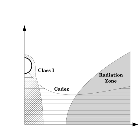
To provide more stable evolutions, especially for the widely separated black hole cases, we utilize a coordinate “patch” as described in Paper II. Evolutions in this patched domain, which covers the saddle points and portions of the axis, are performed using the cylindrical coordinate based metric components and chain rule derivatives to compute spatial gradients across the curvilinear grid nodes. The solutions are then transformed using the general tensor relations to reconstruct the curvilinear metric and extrinsic curvature components, and then linearly blending the results into the rest of the spacetime, which is evolved in a normal manner using the curvilinear metric components on the curvilinear grid. The coordinate patch used in Papers I–III, although only several zones deep in the angular direction, extends from the throat all the way out to the outer boundary in the radial direction. For comparison (see Fig. IV A), the domain in the class I coordinates which requires a patch is localized to just the first few zones in the radial direction. As a result, when the black holes merge to form a common event horizon, the patched coordinates and the associated numerical evolutions become irrelevant as the lapse collapses to zero over this region before the metric shear grows enough to disrupt the solutions. The evolutions with class I coordinates are therefore more robust and less sensitive to patch parameters then previous calculations. FIG. 8.: Locations, shapes and sizes of the coordinate patches used in the Misner $\mu=2.7$ grids for the Čadež (horizontally hatched domain) and class I (diagonally hatched domain) cases. The shaded region labeled “radiation zone” represents the domain into which most of the gravitational radiation is emitted. That this zone is concentrated along the equator is attributed to the axisymmetric nature of the collision. Despite the representative shape of the radiation zone, the actual radiation extraction is performed on 2–spheres starting at a radius of 30$M$ (= 15$M_{ADM}$) from the origin.
 

B Results

FIG. 9.: Gravitational waveforms emitted from the head–on collision of two black holes evolved with the Čadež and class I grids for the $\mu=$ 1.6, 2.2 and 3.0 Misner data. The waveforms are extracted at a radius of 30$M$ from the origin, where $M=M_{ADM}/2$ is the approximate single black hole mass. The evolutions in each case are performed at a grid resolution of 200$\times$35 (radial$\times$angular) cells.
 

We first consider three different cases with Misner parameters $\mu=$ 1.6, 2.2, and 3.0, and compare the class I gravitational waveforms with previous results using the Čadež grid. Each calculation is performed at the same grid resolution using 200$\times$35 radial$\times$angular zones. The Misner parameters are chosen so that the smaller value represents a data set in which the two black holes are already merged within a single event horizon, and the subsequent evolution is that of a single distorted black hole ringing down to the Schwarzschild solution as it emits gravitational waves. The data from the larger Misner parameter cases correspond to two distinct black holes separated by proper distances of $L=8.92M$ ($\mu=2.2$) and $L=15.8M$ ($\mu=3.0$) between the two throats, where $M$ is half the ADM mass of the spacetime (or approximately the mass of a single black hole). Comparison plots of the dominant $\ell=2$ Zerilli waveforms, extracted at a distance of 30$M$ from the origin, are shown in Fig. IV B for the three different Misner cases. We find maximum relative differences less than about 10% in amplitude and 4% in phase for the $\mu=$ 1.6 and 2.2 cases (with absolute deviations $<10^{-2}$ in amplitude), and up to about 200% and 4% differences in amplitude and phase for the more difficult $\mu=$ 3.0 case in which the black holes are initially highly separated.

To emphasize the (in)stability of the solutions at late times when the signal crossing the detector becomes weaker, we plot in Fig. IV B the logarithm of the absolute value of the Zerilli function for the relatively uncertain $\mu=3.0$ case. Notice the class I grid solution maintains a more regular oscillatory behavior and consistent damping rate throughout the wave signal and for longer periods of time than the Čadež case, which begins to break down at about 70$M_{ADM}$.

FIG. 10.: The absolute value of the Zerilli function is shown for the $\mu=3.0$ case using the class I and Čadež grids. The logarithmic scale highlights the oscillations in the waveform and the exponential damping of the wave amplitude. Although the waveforms compare favorably at smaller values of $\mu$, there is a significant difference and improvement in the regularity of oscillations in the class I system compared with the less stable Čadež case for this large initial separation data.
 

Next, we reproduce in Fig. IV B the equivalent of Fig. 14 in Paper III. The total $\ell=2$ radiated energy (in units of the ADM mass, $M_{ADM}=2M$) emitted during the black hole collisions is plotted as a function of the initial separation distance (in units of $M$) between the two throats. Also included in the figure are results from Paper III, the Davies et al. [13] (DRPP) point particle calculation ($E=0.0104m^{2}/M$, plotted for $m=M=M_{ADM}/2$), and its reduced mass correction ($m\rightarrow mM/(m+M)$). Results from the class I and Čadež grid evolutions match extremely well, better than 3%, for separation parameters $\mu\leq 2.2$ corresponding to initial physical separations of $L\leq 8.92M$, and improve significantly at smaller $\mu$ values. However, deviations between the class I and Čadež results become greater for black holes with further initial separations, reflecting the difficulty in evolving highly separated black holes for long periods of time.

To assert a measure of uncertainty in our results, we perform several different calculations of the $\mu=2.7$ and 3.0 data, varying the grid resolution, patch width, and coordinate parameters as defined in Sec. II A to manipulate the shape of the coordinate lines. For the more problematic Čadež evolutions, additional parameters include the patch length, duration and diffusion, as well as varied treatments of the coordinate singularity (for example, shift vector specifications, discretization stencils, and regularization of certain metric and curvature components). The symbols in Fig. IV B represent the median results and the error bars indicate the variance with computational parameters. The variances are similar to the differences observed between the Čadež and class I results: roughly 30% and 100% in the $\mu=2.7$ and 3.0 cases respectively, with a trend for better agreement with increased resolution (though the resolution studies are limited by the axis instability). For the $\mu\leq 2.2$ cases the variances are too small to plot, but are consistent with the observed agreement in the evolutions. Considering the sensitivity of the results to grid and patch parameters, and the difficulties in evolving these systems using maximal slicing conditions and in axisymmetry, the overall results agree fairly well. Furthermore, the numerical calculations are in reasonable agreement with the reduced mass approximation and the semi–analytical calculation of Araújo and Oliveira [14] in the large separation limit.

FIG. 11.: Total gravitational wave energy (in units of the ADM mass) emitted from the head–on collision of two equal mass black holes as a function of the separation distance between the two throats (in units of $M=M_{ADM}/2$). The class I and Čadež grid results are plotted together for comparison, along with the DRPP [13] calculation of a particle falling into a more massive black hole, and its reduced mass correction. The error bars represent the uncertainties estimated by performing the evolutions for different computational parameters as described in the text. The uncertainties in both the class I and Čadež evolutions are comparable to differences between the two different grid results, ranging from $<3$% for separations $L<10M$, 30% for $L\sim 13M$, and 100% for $L\sim 16M$.
 

Fig. IV B also demonstrates an added advantage of the new grid generation procedure to construct numerical grids in the very low Misner parameter cases. Due to convergence problems in the Newton–Raphson iterative inversion of Eqn. (25) when the black hole throats are placed too close to the saddle point, previous calculations were limited to $\mu\geq 0.7$ [15]. The closest separation data shown in Fig. IV B corresponds to $\mu=0.5$ (or $L=2.51M$), although grids for even smaller values of $\mu$ can be easily generated.

An additional benefit from these new coordinates is their regularity at the origin, which makes calculations of the event horizon and null generators more accurate as the black holes merge. In Fig. IV B we show the evolution of the embedding of the event horizon found in the $\mu=2.2$ case evolved with the class I coordinates. The embedding of the horizon is smooth (except at the cusps on the $z$–axis), as were previous embeddings of the horizon in this spacetime [16]. However, the null surfaces on the class I grid contain not only the horizon (in the domain $\eta>0$), but also naturally contain the locus of generators waiting to find the horizon, as discussed in [17]. More precisely, to generate Fig. 11 of [17] a coordinate transformation from Čadež to $(\rho,z)$ coordinates was required. This coordinate transformation is not needed to evolve the locus in class I coordinates. This is more than a convenience, however. Since the null surface consisting of the horizon plus locus is naturally represented as a smooth continuous surface in Class I coordinates, the entire null surface can be unambiguously embedded in 3–space, which was not possible with the Čadež grid. This allows us to determine the separation between the horizons in embedded space using some relevant physical measure. While in Čadež coordinates the horizon separation was determined to keep the outer surface of the “pair of pants” figure smooth, here we determine the separation by embedding the entire null surface. This gives a natural separation between the horizons from the embedding of the locus and determines the geometry by the horizon. We use this separation to place the holes in the “wristwatch” (or “pair of pants from above”) Fig. IV B. The class I coordinates also allow for more detailed examinations of the caustic line at the coalescence point, which will be discussed elsewhere.

FIG. 12.: Embedding of the event horizon for the $\mu=2.2$ Misner data with the class I evolution. The geometry of the class I coordinates allows the separation between the holes in this figure to be physical, not artificial as in previous two black hole collision embedding diagrams derived from Cadez coordinates. Also, the regularity of the class I grid at the origin allows for more accurate examinations of the caustic line at the coalescence point.
 

V Conclusions

In many ways the axisymmetric evolution of two colliding black holes has been stalled due to the lack of a coordinate system without pathological instabilities or grid singularities. By developing new techniques to generate alternative grids, and by creating body–fitting grid geometries with singularities on the throats of the two black holes, we are able to achieve more stable long time evolutions of two black hole systems. We have demonstrated the applicability of these new grids in actual numerical evolutions of Misner’s initial data set for the head–on collision of two equal mass black holes. The calculations presented here confirm the existing results to fairly good accuracy in the restricted stable parameter range, with maximum relative deviations less than 3% in the radiated energies for the $\mu\leq 2.2$ cases corresponding to initial proper separation distances of $L\leq 8.92M$ (with significantly smaller deviations for the lower $\mu$ cases). The differences increase to about 30% for $\mu=2.7$ ($L=12.7M$) and 100% for $\mu=3.0$ ($L=15.8M$), which are comparable to the uncertainties in the evolutions as defined in Sec. IV B for both the Čadež and class I systems. These differences reflect the difficulty in evolving black holes for long periods of time with maximal slicing conditions, and the sensitivity of the evolutions to treatments of the axis instability and coordinate singularities.

Basically the Čadež and class I evolutions yield consistent results, even at the high $\mu$ values, especially when considering the changes observed in waveforms and energies by varying the computational parameters. In addition to confirming previous results, and because no specialized treatment of the coordinate singularities is required, it seems promising that we can evolve physical systems with these new coordinates which were not as easily addressable with previous codes using either the Čadež or cylindrical coordinate systems. For example, we are currently extending this work to evolve spinning black hole and unequal mass black hole collisions.

To conclude, we emphasize the following advantages of these new coordinates: (1) they achieve better zone coverage in the strong field interaction region near the origin – caustics, photon generators and embeddings of the event horizon are better resolved; (2) the coordinate patch extends over a much smaller domain in the class I system – just a few zones radially, and localized to the $z$–axis – so it is not an unstabilizing element at late times; (3) the resulting gravitational waveforms from evolutions are not as sensitive to the patch parameters, such as its width, length, duration and diffusion parameters; (4) due to its robustness and lack of a need for specialized treatments of the saddle points, the new code is more simplified and easily generalizable to include non-equal mass black holes and spinning black hole collisions; and (5) the new coordinates allow a larger range of initial data in the Misner parameter to be evolved, including evolutions of black holes that are further separated (though the accuracy is questionable for $\mu\geq 3.0$), and more closely spaced (for smaller order perturbations) than in previous calculations. In addition, the new coordinates offer all the same advantages as the Čadež coordinates: They are logarithmic in the radial direction, and spherical on the throat and in the asymptotic wave zone, thus allowing for the same simplified treatment of boundary conditions and waveform extraction.

- [1] S. G. Hahn and R. W. Lindquist, Ann. Phys. (N.Y.), 29, 304 (1964).
- [2] A. Čadež, Ph.D. thesis, University of North Carolina at Chapel Hill, (1971).
- [3] L. Smarr, Ph.D. thesis, University of Texas, Austin, (1975).
- [4] K. Eppley, Ph.D. thesis, Princeton University, (1975).
- [5] L. Smarr, A. Čadež, B. DeWitt and K. Eppley, Phys. Rev. D 14, 2443, (1976).
- [6] C. Misner, Phys. Rev. D. 118, 1110 (1960).
- [7] A. Einstein and N. Rosen, Phys. Rev. 48, 73 (1935).
- [8] L. Smarr, in Sources of Gravitational Radiation, edited by L. Smarr (Cambridge University Press, Cambridge, 1979), p. 245.
- [9] P. Anninos, D. Hobill, E. Seidel, L. Smarr, and W.–M. Suen, Phys. Rev. Lett. 71, 2851 (1993, Paper I).
- [10] P. Anninos, D. Hobill, E. Seidel, L. Smarr, and W.–M. Suen, Technical Report 024, National Center for Supercomputing Applications, (1994, Paper II).
- [11] P. Anninos, D. Hobill, E. Seidel, L. Smarr, and W.–M. Suen, Phys. Rev. D 52, 2044 (1995, Paper III).
- [12] J. F. Thompson, Z. U. A. Warsi and C. W. Mastin, J. Comp. Phys. 47, 1 (1982).
- [13] M. Davis, R. Ruffini, H. Press, and R. H. Price, Phys. Rev. Lett. 27, 1466 (1971).
- [14] M.E. Araújo and S.R. Oliveira, Phys. Rev. D 52, 816 (1995).
- [15] P. Anninos, R.H. Price, J. Pullin, E. Seidel, W.M. Suen, Phys. Rev. D 52, 4462 (1995).
- [16] R. Matzner, H. E. Seidel, S. L. Shapiro, L. Smarr, W.-M. Suen, S. A. Teukolsky, J. Winicour, Science 270, 941 (1995).
- [17] J. Libson, J. Massó, E. Seidel, W.-M. Suen and P. Walker, Phys. Rev. D 53, 4335 (1996).