Phenomenology of the Gowdy Universe on ††thanks: e-mail: berger@oakland.edu, garfinkl@oakland.edu
Abstract
Numerical studies of the plane symmetric, vacuum Gowdy universe on yield strong support for the conjectured asymptotically velocity term dominated (AVTD) behavior of its evolution toward the singularity except, perhaps, at isolated spatial points. A generic solution is characterized by spiky features and apparent “discontinuities” in the wave amplitudes. It is shown that the nonlinear terms in the wave equations drive the system generically to the “small velocity” AVTD regime and that the spiky features are caused by the absence of these terms at isolated spatial points.
98.80.Dr, 04.20.J
I Introduction
Spatially inhomogeneous cosmologies constitute almost a “terra incognita” for general relativity. In particular, the nature of the singularity in generic cosmologies is unknown although Belinskii, Khalatnikov, and Lifshitz (BKL) have conjectured that it is locally Mixmaster-like [1]. Spatially homogeneous universes’ approach to the singularity can be either asymptotically velocity term dominated (AVTD) [2, 3] or Mixmaster-like [1, 4]. In general, AVTD singularities occur when the influence of spatial derivatives can be neglected. This means that the solution to the full Einstein equations eventually comes arbitrarily close to the solution to the truncated equations one obtains by eliminating the terms containing spatial derivatives [3]. In spatially homogeneous models, spatial derivatives in the metric create the spatial scalar curvature which appears as a potential in minisuperspace [4, 5]. An AVTD homogeneous cosmology eventually evolves toward the singularity as a Kasner solution. (The Kasner universe is an exact solution of the vacuum Einstein equations characterized by different expansion rates in different directions with flat spacelike hypersurfaces [6].) Mixmaster dynamics describes the evolution (of non-flat space-like hypersurfaces) toward the singularity as an infinite sequence of (approximately) Kasner epochs. The Kasner indices (which determine the anisotropic expansion rates) change whenever the influence of the spatial scalar curvature reappears. Its recurring influence means that the Mixmaster singularity is not AVTD. BKL claimed to prove that the generic singularity in Einstein’s equations and, in particular, in spatially inhomogeneous cosmologies is Mixmaster-like. While this result remains controversial [7], it provides a conjecture which can be tested by evolving spatially inhomogeneous collapsing universes numerically.
As part of such a study of this issue [8, 9, 10], we have considered the Gowdy universes on as a test case. These models are one of the classes discovered by Gowdy [11, 12, 13] as a reinterpretation of Einstein-Rosen waves [14]. While their plane symmetry precludes local Mixmaster behavior, their nonlinear gravitational wave interactions lead to an interesting phenomenology which forms the subject of this paper. The Gowdy singularity has been conjectured to be asymptotically velocity term dominated (AVTD) [15] and has been shown rigorously to be so for the polarized case [3]. In addition, it has been shown that for the polarized case, cosmic censorship holds: There exists a natural foliation labeled by such that regular initial data evolve without singularity for all where (in the collapse direction) a curvature singularity occurs at [16]. Here we shall use numerical studies to provide support for the extension of the polarized Gowdy results to generic Gowdy models.
Gowdy cosmologies represent the simplest spatially inhomogeneous cosmological solutions to Einstein’s equations. The vacuum case may be interpreted as the two polarizations of gravitational waves propagating in an inhomogeneous background spacetime [8, 12]. The model is plane symmetric with the propagation direction of the waves orthogonal to the symmetry plane. Near the singularity, the metric may be rewritten as locally Kasner with spatially dependent Kasner indices [12]. (This is a non-rigorous statement of AVTD behavior.). Matter fields compatible with the Gowdy metric have been discussed by Carmeli, Charach, and Malin [17, 18], and Ryan [19]. Here we shall consider only vacuum solutions.
The main phenomena of interest in the Gowdy universe are the growth of small scale spatial structure and the approach to the AVTD regime. We shall demonstrate that both result from the nonlinear terms in the wave equation for , the polarization of the gravitational waves. These act as space and time dependent potentials whose effect is to drive the system to velocity dominance. As the AVTD regime is reached, the potentials approach zero. Their spatial dependence means that wave amplitudes grow at some spatial points and decrease at others, eventually producing small scale spatial dependence in the waveforms. Non-generic behavior occurs at points where the coefficients of the potentials (separately) vanish identically. We note that this analysis in terms of potentials explains the observed episodic evolution of the system to the AVTD regime and the fact that the conditions for AVTD are reached at some spatial points before others. This should be considered together with the asymptotic expansion developed by Grubis̆ić and Moncrief (GM) [15] which displays an exponential decay to the AVTD limit, applicable in the last episode.
The primary advantage of the Gowdy models as a test case for the study of inhomogeneous cosmologies is the existence of variables in which the dynamical equations for the wave amplitudes decouple from the constraints. Initial data for the wave equations may be freely specified (restricted only in that the total momentum along the direction of propagation must vanish) while the constraints appear as prescriptions for the construction of the background metric from the known solution to the dynamical equations. Thus the two principal difficulties of numerical relativity—solving the initial value problem and preserving the constraints during the evolution—become trivial. This decoupling between dynamical and constraint equations disappears in more complicated inhomogeneous models. However, studies of symmetric cosmologies (with only one Killing field) indicate that many features of the Gowdy phenomenology such as spiky small scale spatial structure persist in these more complicated models [8, 20, 10] and, presumably, would be important in the dynamics of generic cosmologies.
In Section 2, the Gowdy model on will be reviewed. Section 3 will contain a brief description of the numerical method. In Section 4, the phenomenology will be described. Section 5 will contain a unified explanation for the phenomenology. Discussion will be given in Section 6.
II The Model
The Gowdy model on is described by the metric [11, 8]
| (2) | |||||
where , , are functions of , . The sign of differs from that in [8] as required for consistency with the form given there for the equations for . The arguments in [8] did not depend on this error. We impose spatial topology by requiring and the metric functions to be periodic in . If we assume and to be small, we find them to be respectively the amplitudes of the and polarizations of the gravitational waves with describing the background in which they propagate. The time variable measures the area in the symmetry plane with a curvature singularity. Einstein’s equations split into two groups. The first is nonlinearly coupled wave equations for and (where ):
| (3) |
| (4) |
The second contains the Hamiltonian and -momentum constraints which can be expressed as first order equations for in terms of and :
| (5) |
| (6) |
This split into dynamical and constraint equations removes two of the most problematical areas of numerical relativity from this model: (1) The normally difficult initial value problem becomes trivial since , and their first time derivatives may be specified arbitrarily. The only restriction, that the total momentum in the waves vanishes, is a consequence of the requirement that metric variables be periodic in . (2) The constraints, while guaranteed to be preserved in an analytic evolution by the Bianchi identities, are not automatically preserved in a numerical evolution with Einstein’s equations in differenced form. However, in the Gowdy model, the constraints are trivial since may be constructed from the numerically determined and . For the special case of the polarized Gowdy model (), satisfies a linear wave equation whose exact solution is well-known [12]. For this case, it has been proven that the approach to the singularity is AVTD [3]. This has also been conjectured to be true for generic Gowdy models [15]. We shall show in Section 5 how a numerical study of this model provides strong support for this conjecture.
The wave equations (3) and (4) can be obtained by variation of the Hamiltonian [13]
| (7) | |||||
| (8) |
The variation of the kinetic energy term, , yields equations of motion for the AVTD solution which arises when spatial derivatives are neglected. These equations are exactly solvable with the solution
| (9) | |||||
| (10) | |||||
| (11) | |||||
| (12) |
given in terms of four functions of : , , , and . Here . The large limits given above are for . The special case will be discussed later. While (9) may be solved for all these functions, it is convenient to note that [15]
| (13) |
is the geodesic velocity in the target space (with metric ) of the wavemap [13, 15, 8]. If, as the singularity is approached, the behavior is AVTD, the true solution will approach the AVTD one. The exponential prefactor in of (7) makes plausible the conjectured AVTD singularity. However, (for ) as . If , the term in can grow rather than decay as . In fact, if one assumes the AVTD behavior as in (9), the wave equations become [15]
| (14) | |||||
| (15) |
where . These equations are inconsistent if unless , which does not occur in a generic (unpolarized) Gowdy model. However, in generic Gowdy models, one also expects isolated points (a set of measure zero) with but . In Section 5, we shall see that can persist at such isolated values of where the AVTD conditions may not be satisfied. GM thus conjecture that the AVTD limit as requires everywhere except, perhaps, at a set of measure zero (isolated values of ) [15]. We note that the polarized Gowdy model () has the AVTD solution , with unrestricted in sign or magnitude [12, 3]. The fact that this behavior is not a limit of the generic AVTD solution (9) illustrates further the qualitative distinction between the polarized case and but arbitrarily small.
III Numerical Methods
The numerical method is discussed in detail elsewhere [8]. However, we shall summarize it here. The work reported here was performed by using a symplectic PDE solver[21, 22]. Consider a system with one degree of freedom described by and its canonically conjugate momentum with a Hamiltonian
| (16) |
Note that the subhamiltonians and separately yield equations of motion which are exactly solvable no matter the form of . Variation of yields , with solution
| (17) |
Variation of yields , with solution
| (18) |
Note that the absence of momenta in makes (18) exact for any . One can then demonstrate that to evolve from to an evolution operator can be constructed from the evolution sub-operators and obtained from (17) and (18). One can show that [21]
| (19) |
reproduces the true evolution operator through order . Suzuki has developed a prescription to represent the full evolution operator to arbitrary order [23]. For example
| (20) |
where . The advantage of Suzuki’s approach is that one only needs to construct explicitly. is then constructed from appropriate combinations of .
The generalization of this method to degrees of freedom and to fields is straightforward. In the latter case, so that becomes the functional derivative . On the computational spatial lattice, the derivatives that are obtained in the expression for the functional derivative must be represented in differenced form. We note that, to preserve th order accuracy in time, th order accurate spatial differencing is required. Some discussion of this has been given elsewhere [8].
Convergence studies have been performed to test the algorithm. We have already shown [8] that at any fixed value of , there exists a spatial resolution at which every spiky feature is resolved. Any finer resolution will yield identical results. However, as we shall see, generic spiky features grow narrower as the singularity is approached. This means (see [8]) that a spatial resolution which was adequate at some will fail to resolve all features at some . This type of “resolution dependence” is well understood to be a consequence of the physical behavior of the model. If the physical system has features which become arbitrarily narrow as , no resolution will be adequate everywhere for all time.
IV Gowdy Phenomenology
Here we report the results of a numerical study of the evolution of generic Gowdy models toward the singularity (). Rather than perform simulations for hundreds of Gowdy models, we consider a single class of models and argue that the observed behavior is generic. For the most part, we shall use the initial data , , , and . This model is actually generic for the following reasons: The dependence is the smoothest nontrivial possibility. Since we shall discuss the growth of small scale spatial structure, we expect the cleanest effects to arise from the smoothest initial data. A more complicated initial state will not yield any qualitatively new phenomena. For example, choosing instead yields the same solution repeated times on the grid thus yielding the same result with poorer resolution. In addition, the amplitude of is irrelevant since the Hamiltonian (7) is invariant under , for any constant . This also means that any unpolarized model is qualitatively different from a polarized () one no matter how small . Traveling waves (subject to where is the total -momentum) yield qualitatively similar behavior [24]. We are interested in the spatial structure that can develop from smooth initial data. For this reason, we have used spatial dependence. Starting with a more complicated wave form will yield an eventually more complicated spatial structure but nothing qualitatively different will appear. Similarly, since rescaling does not change the solution qualitatively, the amplitude of is kept fixed. In this discussion, we shall consider only and and construct later if desired.
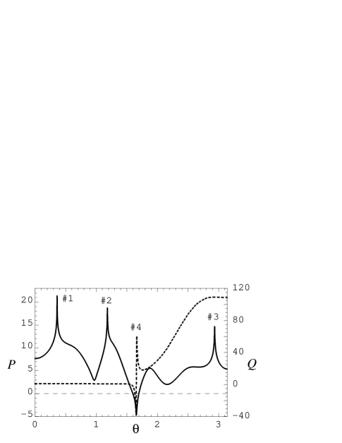
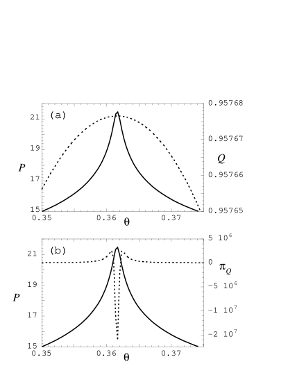
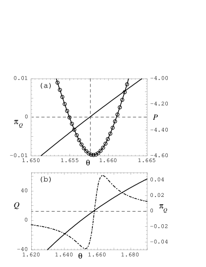
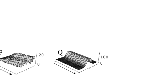
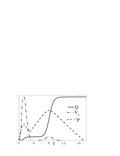
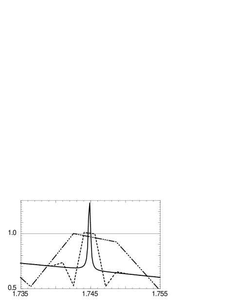
From the chosen class of initial data, with high spatial resolution, one obtains after some time () the profiles for and shown in Fig. 1. The numbered features are typical for any generic solution. The peaks labeled #1, #2, and #3 arise from the same features of the nonlinear interactions. On a finer spatial scale in Fig. 2, we notice that (a) the peak in is associated with an extremum of (which may be a maximum or minimum) and (b) becomes large with for a maximum (minimum) in . The apparent discontinuity in (labeled #4 in Fig. 1) is shown on a finer scale in Fig. 3. We see that this feature occurs as goes through zero where . In Fig. 4, the same features #1 and #4 are shown at . We see that the “spikes” have narrowed in .
The evolution of and is shown in Fig. 5 (see also [8]) where it is clearly seen that ever shorter wavelength modes develop until the point at which the AVTD behavior sets in. Fig. 6 shows an interesting self-similarity in the early evolution. The parameter in the initial data is varied in a sequence of simulations. In each case, the number of peaks in is counted after each time step. We find
| (21) |
where is the time at which peaks are first present in the waveform and is a constant. From (21), denotes the value of such that the th peak appears only at . The scaling shown in Fig. 6 is for . Similar (but less accurate) straight line fits are found for equal 3 and 7. (The wave equations are even in as are the initial data so that and remain even functions of . Thus, except for a central peak, other peaks will form two at a time.)
Thus, one may summarize that spatial structure forms more rapidly and evolves a more complicated form, the greater the initial “energy” in the waves as denoted by, e.g., from (13). Eventually, the waveforms of and “freeze” to the AVTD behavior of increasing linearly and constant in . As has been emphasized by Hern and Stuart (HS) [25], the duration in of the observed non-AVTD regime depends on the spatial resolution of the simulation.
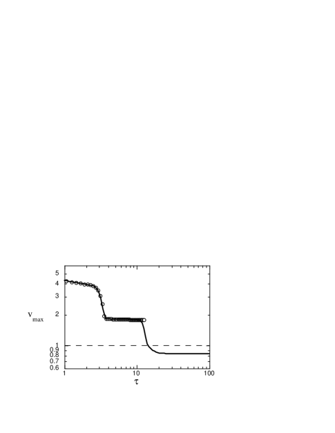
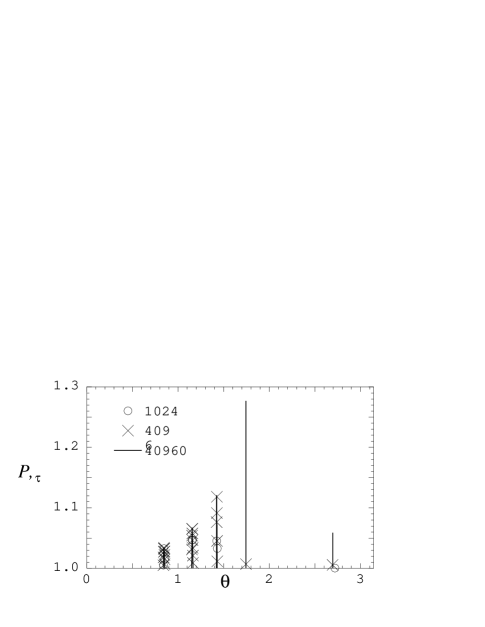
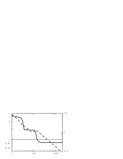
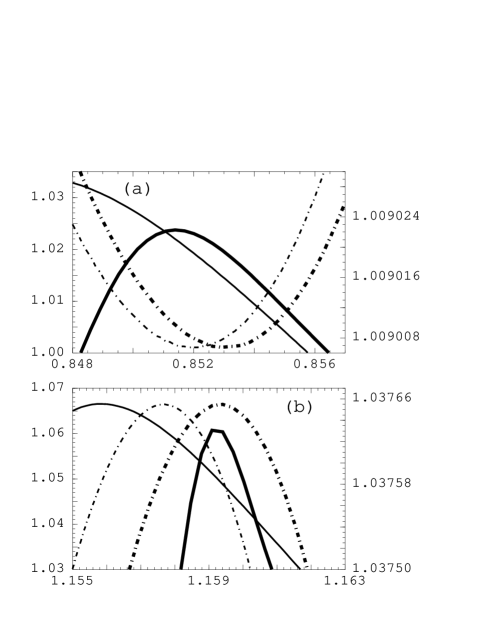
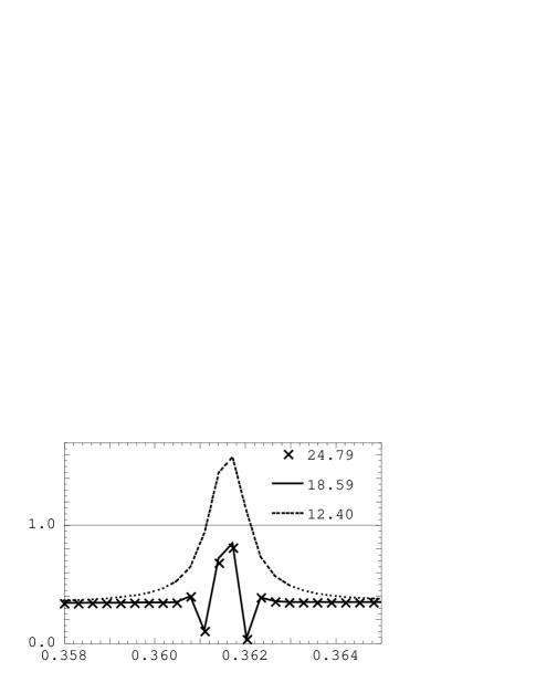
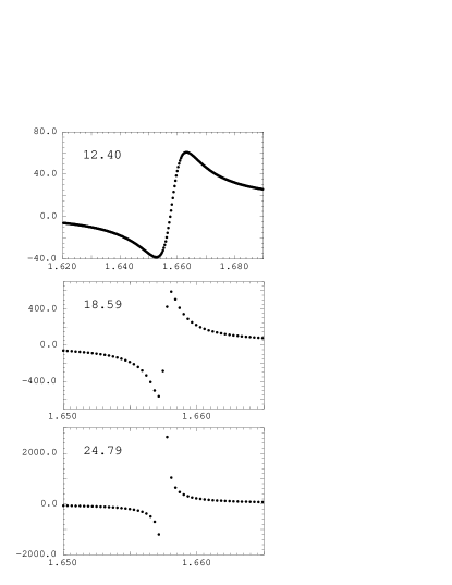
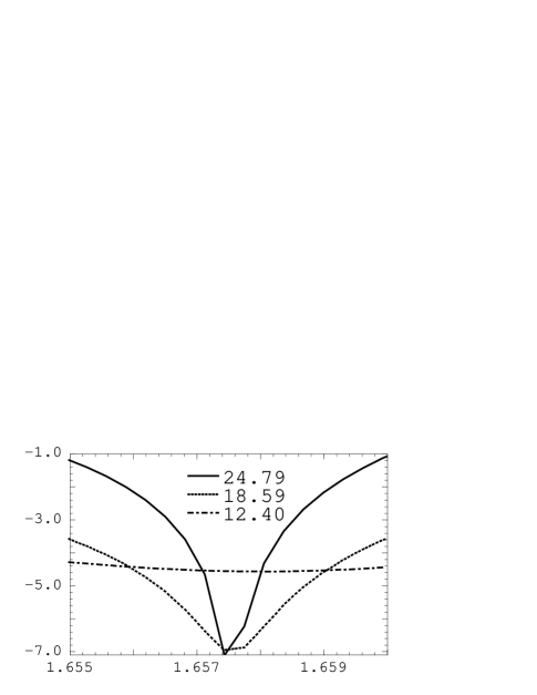
In Fig. 7, the maximum value over the spatial grid, , of the AVTD parameter is shown as a function of time for two simulations with different spatial resolutions. The steps in occur when the location of the spatial point with the maximum value of changes. Note that, for the lower resolution simulation, eventually falls below unity in support of the GM conjecture [15]. We also see that the higher resolution simulation starts to diverge from the lower resolution one, signaling the presence of narrow features that are unresolved by the coarser resolution. (The former was not run longer primarily because the Courant condition requires small time steps for high resolution studies.) This suggests (as confirmed by HS) that the higher spatial resolution simulation will take longer before it becomes AVTD everywhere. This is shown explicitly in Fig. 8 where vs is plotted for three different spatial resolutions. Note that for two of the spikes, is larger for the finest resolution. In Fig. 9, the difference between and is plotted vs. . Since as , we see the influence of the next (constant in ) term , in the AVTD solution for (9).
V Structure in the Gowdy Model
To understand the Gowdy phenomenology of Section III, we must explore the structure of the wave equations for and . Let us consider (4) first. The equation for may be rewritten in first order form as
| (22) | |||||
| (23) |
This immediately provides the explantion for both the large central peak which quickly forms in and for the apparent discontinuity in seen in Figs. 1 and 3. From (22), will grow rapidly where is negative. Since, early in the evolution, , one expects a large peak (as is observed in Figs. 1 and 5) where . We shall see later that is driven to positive values eventually stopping the growth of . However, we shall also see that if , can remain negative longer. Say for at a value of where . Thus we find that
| (24) |
so that is large and increases (decreases) exponentially depending (say for ) on whether . Note that we assume . However, (22b) implies this for large and negative.
More interesting is the equation for . Consider two approximate forms of (3) depending on which nonlinear term dominates. Since the nonlinear terms depend exponentially on , they will dominate the linear spatial derivative term when the exponential is large.
For example, if is large and negative,
| (25) |
which has the first integral
| (26) |
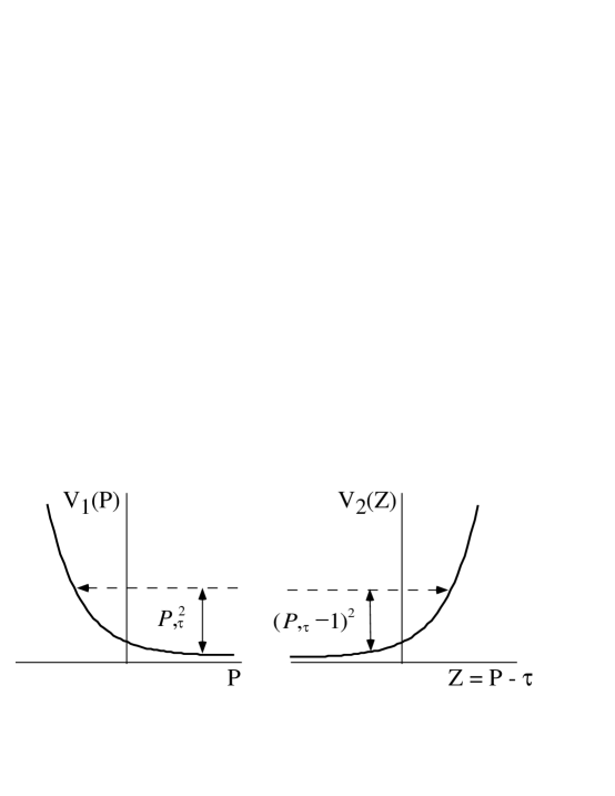
This allows one to define an effective potential
| (27) |
which is important when and (especially if) . This allows immediate explanation of the following phenomena: (a) In the AVTD regime, and its asymptotic time derivative since if , a bounce off will occur at which so that will eventually reach positive values. (b) However, if , so that both and can remain negative for a long time. Non-generic behavior occurs at the isolated point where vanishes since and will never be driven to positive values there.
On the other hand, if (a) is large and positive and (b) , the wave equation for is given by
| (28) |
which is easy to integrate (for ) as
| (29) |
Thus if , the dynamics of is dominated by an effective potential
| (30) |
Again, from (22a), our implicit assumption that is consistent. One sees immediately, that if a bounce off will occur with the result that or
| (31) |
Thus the existence of provides a mechanism to drive and thus asymptotically to values below unity. In the actual simulation, the asymptotic regions for the scattering are not reached so that (31) cannot be used to compute the numerical value of the change in with . Again one sees that non-generic behavior can arise, in this case, at where . At the mechanism to drive below unity is absent so that larger values of are allowed. If is non-vanishing but small, it will take a long time for the bounce to occur so that the AVTD limit will take a long time to arise. This also explains the peaks in seen in Fig. 1. Where , is small so that can increase without hindrance with a large positive value of .
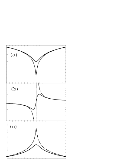
For a more quantitative understanding of the small scale spatial structure, note that both equations (18) and (21) have closed form solutions. Equation (18) holds in the AVTD regime, where the solution is given in equation (7). The exceptional point is the point where . Near this point we have where . It then follows that for large
| (32) | |||
| (33) |
Thus there is a spiky feature in both and at as is shown in Fig. 10. Furthermore, these features steepen exponentially with time. Because of this steepening, the spatial derivatives of and become large at late times. However, the AVTD equations are formed by dropping spatial derivatives from the exact equations (2) and (3). Therefore, one might worry that the terms that have been neglected are not actually negligible near the peaks. However, using equation (14) one can show that near the neglected terms go like and are therefore exponentially damped for .
The solution of equation (21) is
| (34) |
Here, , and are functions of , and . Note that for large where . The exceptional point is the point where . Near this point we have where . It then follows that for large
| (35) |
Thus the feature in narrows exponentially with time as can be seen in Fig. 10. The spatial derivatives of become very large. However, the neglected terms in the equations go like . Since for asymptotically, it follows that these terms become negligible after the last bounce.
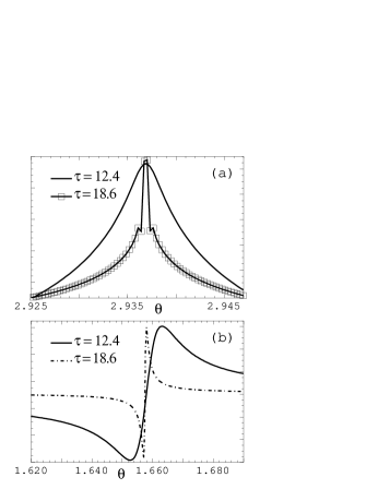
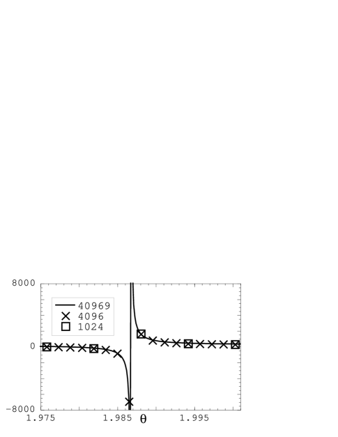
The differences in Figs. 7 and 8 seen by increasing the spatial resolution are also understood in terms of our analysis of structure growth. At higher spatial resolution it is more likely that a spatial grid point of the numerical simulation will be very close to a non-generic point where . Thus the non-generic behavior will become more apparent and the time to reach the AVTD limit characterized by everywhere will be longer. Clearly, the observed resolution dependence may be interpreted to be evidence for the existence of non-generic points. The apparent discontinuity in seen in Figs. 1 and 3 is evidence for the non-generic point in where . Its effect may be seen as a resolution dependence of the shape of this feature. It becomes steeper and narrower with increasing spatial resolution for sufficiently large (see Fig. 11) or for increasing with fixed spatial resolution (see Fig. 4b). As in Fig. 2, we note that the spikes in Fig. 8 where are associated with extrema in . This is shown in Fig. 12. Note that the alignment is not perfect between the peak in and the extremum in where the spike is well resolved (see also Fig. 3a). This is understood as evidence that the AVTD regime has not yet been reached. In particular, the site of the extremum may be distorted by a nearby larger feature in . Running the simulation twice as long (Fig. 13) shows much closer alignment and is evidence that the predicted non-generic behavior will eventually dominate the spikes.
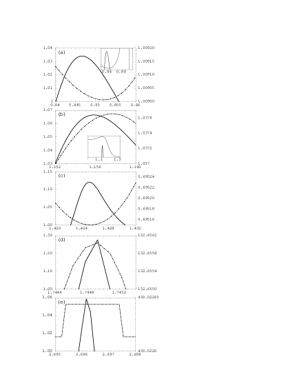
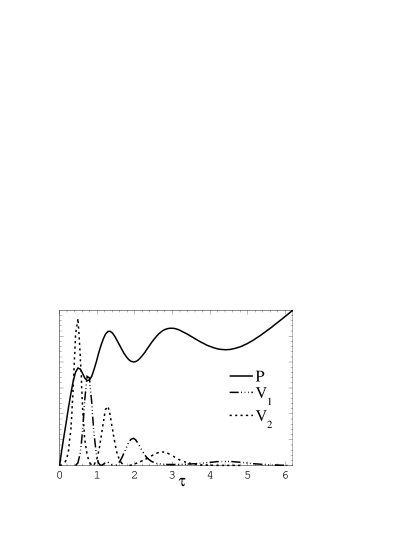
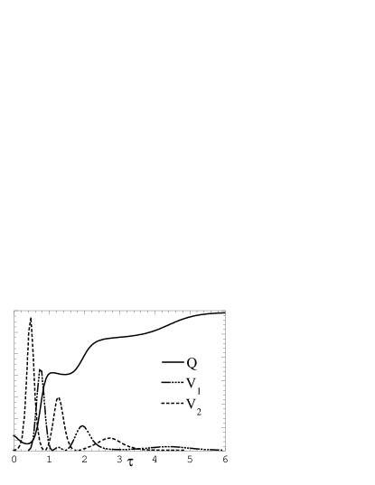
The effective potentials and are displayed in Fig. 14. We see that the approach to the AVTD regime is characterized by repeated alternate interactions of with the two potentials. This is displayed explicitly for a typical value of in Fig. 15 where , , and are shown as functions of . After each interaction with , the quantity changes sign. If this yields , no further bounces occur. If , there will be an interaction with . Eventually, falls below unity so that permanently disappears. then continues to increase for all subsequent with constant slope as is characteristic of the AVTD limit. (Note that will also decrease exponentially as increases even though it is part of the AVTD solution.) Examination of (22) shows that, when falls below unity and , as required by the AVTD limit. Once becomes constant, as increases, , again as required. The development of with time is shown in Fig. 16 for the same value of as in the previous figure. Here we see clearly how grows fastest when dominates. This becomes even more dramatic in Fig. 17 which is the same graph for , the site of the apparent discontinuity in .
It is important to emphasize that the magnitude and time evolution of and as well as the initial values of the wave amplitude time derivatives are different at different values of . This explains the development of complicated small scale spatial structure. From (26) or (29), one computes the time to the first bounce off or as
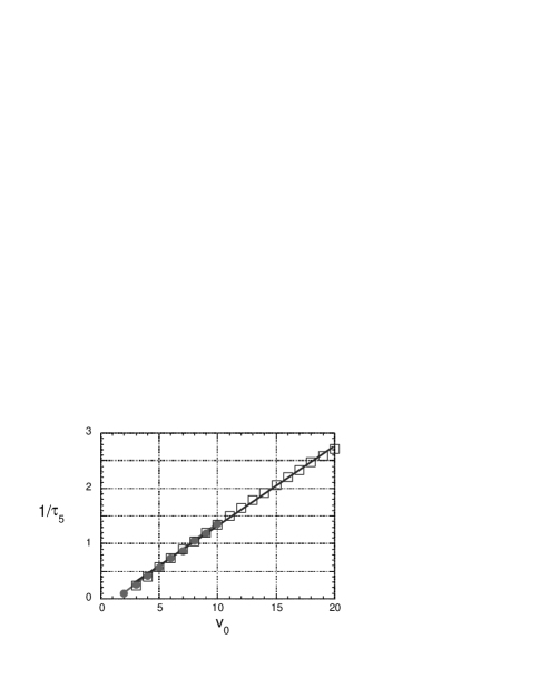
| (36) |
where or and at . Here and . Evaluation of (26) and (29) at yields an approximate inverse scaling with seen in Fig. 6. The central peak appears first and is easy to understand. Since, initially, , the highest negative velocity occurs at causing the bounce off to occur there first. then begins to increase at both earlier and faster than at neighboring values of . More complicated is the next pair of peaks which occur near . Initially, the profile of vs steepens. However, bounces off will begin to occur. This causes the tangent to vs to evolve from negative (positive) to positive (negative) slope for () eventually creating a pair of peaks. The higher the original value of , the greater will be the number of bounces before disappears for good. Ever finer small scale structures are created at values where many bounces occur since will increase for some spatial regions and decrease for others in a manner that changes with time. As falls below unity, at a given , the bounces, and thus structure formation, will cease there but structure formation will continue in the ever smaller spatial regions where continues to exceed unity.
VI Discussion and Conclusions
We see that both potentials and drive the cosmology toward the AVTD regime characterized by (9) as with . This is because appears and influences the dynamics only when and where while does so only for . In the AVTD regime, with , both corresponding terms in the wave equation for are exponentially small. We note that the wave equations (3) and (4) provide no other mechanism to drive into the required range if it is not there initially. Recall that the polarized Gowdy model can have any value for . Thus we argue that at isolated points (a set of measure zero in ) where either or is precisely zero, could remain outside the allowed range. In the former case (say at ), the consistency equations (14) are satisfied so that one expects the solution at to be like an AVTD polarized solution. However, in the latter case (say at ), the consistency conditions require as well as —something one does not expect generically. If at , then the solution is of the AVTD large type there. If , the behavior cannot be analyzed either numerically or by these analytic methods. We may therefore conclude that the simulations provide strong support for the conjecture that the Gowdy models have a singularity which is AVTD except, perhaps, at a set of measure zero.
The existence of this set of measure zero of “non-generic” spatial points can be inferred from the simulations since near them the potentials are very flat. Thus, the closer one is to e.g. or defined as above, the longer it will take to drive to the range there. This manifests itself as a resolution dependence of the simulations of a very specific type. At any value of (say ), there is a spatial resolution sufficient to resolve all spiky features. (This was demonstrated in [8].) But the “center” of each spiky feature is the site of a non-generic point. As one moves away from this point in either direction in , the coefficient of the potential will be larger. Thus the interaction with the potential will occur first at regions away from the center of the feature and move closer to the center as increases. Since the effect of the interaction is to change the sign of either or , the interactions will tend to eliminate the outer part of the spiky feature. Thus the spiky feature gets narrower in time until for some , the original resolution is no longer adequate. Although, in a peak near , should be , inadequate resolution may act as an effective averaging to give a measured smaller value of . Thus the peak in appears to decrease in amplitude only because, at most values, the interaction with has already occurred. We note that this effective averaging will give everywhere for some for any fixed spatial resolution. As the spatial resolution is increased, will also increase since accurate resolution of spiky features can be maintained farther into the simulation and the effective averaging will take longer to come into play. Thus the apparent resolution dependence is consistent with the behavior of the potentials and expected near the non-generic points.
Several examples are shown in Figs. 18–21. In Fig. 18, a spiky feature in is shown for three different spatial resolutions at . While the coarsest resolution shows , it also clearly fails to resolve the spiky feature. The highest resolution both resolves the spiky feature and shows that it has a core where as expected. A similar spiky feature in is shown in Fig. 19 for three different times for the same spatial resolution. One expects that the clearly resolved spike observed early in the simulation will narrow as increases remaining always at the center of the peak. This is not observed (rather one sees the constant behavior expected in the AVTD limit). However, one again sees clearly that the spatial resolution which was adequate at has become inadequate at later times and that the properties of the spike are not correctly represented. Fig. 20 shows that the apparent discontinuity in becomes narrower and steeper with time and eventually is not adequately resolved at a given spatial resolution. One expects to be increasingly negative at the center of this feature since is maintained at that non-generic point. At fixed spatial resolution, we see in Fig. 21 that the negative region of both narrows and deepens as increases from to as expected. However, at , the expected behavior is not seen since the depth of the negative region fails to increase. However, we also see that the spatial resolution has become inadequate. Presumably, adequate spatial resolution would show the narrowness and depth of the negative region suggested by the curvature of vs in the region just outside the core.
In conclusion, the behavior of generic Gowdy cosmologies on can be completely understood in terms of the nonlinear interactions between the two polarizations of the gravitational waves. These act as effective potentials which drive the system to the prediced AVTD behavior and then cease to play a role. At the set of measure zero where the potentials are absent, may lie outside its allowed AVTD range of for all if it does so at any time since the mechanism to correct its value is absent. The existence of this set of measure zero is inferred from the details of the shape and time dependence of the spiky features and from the inability to resolve them with a given spatial resolution beyond a certain time.
Acknowledgements
The authors would like to thank Vincent Moncrief and Boro Grubis̆ić for useful discussions. BKB would like to thank the Institute for Geophysics and Planetary Physics at Lawrence Livermore National Laboratory and the Albert Einstein Institute at Potsdam for hospitality. This work was supported in part by National Science Foundation Grants PHY9507313 and PHY9722039 to Oakland University. Computations were performed at the National Center for Supercomputing Applications (University of Illinois).
REFERENCES
- [1] V.A. Belinskii, E.M. Lifshitz, I.M. Khalatnikov, Sov. Phys. Usp. 13, 745–765 (1971); Adv. Phys. 19, 525–573 (1970).
- [2] D. Eardley, E. Liang, R. Sachs, J. Math. Phys. 13, 99 (1972).
- [3] J. Isenberg, V. Moncrief, Ann. Phys. (N.Y.) 199, 84–122 (1990).
- [4] C.W. Misner, Phys. Rev. Lett. 22, 1071–1074 (1969).
- [5] M.P. Ryan, Jr., L.C. Shepley, Homogeneous Relativistic Cosmologies (Princeton University, Princeton,1975).
- [6] E. Kasner, Am. J. Math 43, 130 (1921).
- [7] J.D. Barrow, F. Tipler, Phys. Rep. 56 372 (1979).
- [8] B.K. Berger, V. Moncrief, Phys. Rev. D 48, 4676 (1993).
- [9] B.K. Berger, in Proceedings of the 14th Internatial Conference on General Relativity and Gravitation, edited by M. Francaviglia, G. Longhi, L. Lusanna, E. Sorace (World Scientific, Singapore, 1997).
- [10] B.K. Berger, D. Garfinkle, V. Moncrief, in Proceedings of the Workshop on Black Hole Interiors, edited by L. Burko, A. Ori (Haifa, 1997), gr-qc/9709073.
- [11] R.H. Gowdy, Phys. Rev. Lett. 27, 826–829 (1971).
- [12] B.K. Berger, Ann. Phys. (N.Y.) 83, 458 (1974).
- [13] V. Moncrief, Ann. Phys. (N.Y.) 132, 87–107 (1981).
- [14] A. Einstein, N.J. Rosen, J. Franklin Inst. 223, 43 (1937).
- [15] B. Grubis̆ić, V. Moncrief, Phys. Rev. D 47, 2371 (1993).
- [16] P.T. Chrusciel, J. Isenberg, V. Moncrief, Class. Quant. Grav. 7, 1671 (1990).
- [17] Ch. Charach, S. Malin, Phys. Rev. D 21, 3284 (1980).
- [18] M. Carmeli, Ch. Charach, S. Malin, Phys. Rep. 76, 79–156 (1981).
- [19] M.P. Ryan, Jr., “Plane-Symmetric Cosmologies—An Overview,” in SILARG, pp. 96–121.
- [20] B.K. Berger, V. Moncrief, “Numerical Evidence for a Velocity Dominated Singularity in Symmetric Cosmologies,” unpublished.
- [21] J.A. Fleck, J. R. Morris, M.D. Feit, Appl. Phys. 10, 129–160 (1976).
- [22] V. Moncrief, Phys. Rev. D 28, 2485–2490 (1983).
- [23] M. Suzuki, Phys. Lett. A146, 319 (1990).
- [24] C.M. Swift, Masters Thesis, Oakland University (1993).
- [25] S.J. Hern, J.M. Stewart, “The Gowdy Cosmologies Revisited,” gr-qc/9708038. (However, see also gr-qc/9708050.)