Dissipative fluids out of hydrostatic equilibrium

Abstract

In the context of the Müller-Israel-Stewart second order phenomenological theory for dissipative fluids, we analyze the effects of thermal conduction and viscosity in a relativistic fluid, just after its departure from hydrostatic equilibrium, on a time scale of the order of relaxation times. Stability and causality conditions are contrasted with conditions for which the ”effective inertial mass” vanishes.

1 Introduction

The study of the evolution of self-gravitating systems (even in the spherically symmetric case) requires the use of numerical procedures and/or the introduction of simplifying assumptions. The former usually lead to model dependent conclusions and the later are frequently too restrictive and/or deprived of physical justification.

An alternative path to this question consists in perturbing the system, compeling it to withdraw from equilibrium state. Evaluating it after its departure from equilibrium, it is possible to study the tendency of the evolution of the object. This is usually done following a first order perturbative method which neglects cuadratic and higher terms in the perturbed quantities. If the relevant processes occuring in the self-gravitating object take place on time scales which are of the order of, or smaller than, hydrostatic time scale, then the quasistatic approximation fails (e.g. during the quick collapse phase preceding neutron star formation). In this case it is necessary to evaluate the system immediately after its departure from equilibrium, where immediately means on a time scale of the order of relaxation times.

This approach has proven to be useful in the dissipationless case [1, 2, 3]. Nevertheless, it has been recently found [4, 5] that for non-viscous dissipative case this approach cannot always be applied. In particular, the goodness of the first order perturbation method can be examined by means of the value of the local parameter

$$\alpha=\frac{\kappa T}{\tau(\rho+p)},$$

where $\kappa$ is the thermal conductivity, $T$ is the temperature, $\tau$ is the relaxation time for thermal signals and $\rho$ and $p$ are the energy density and the radial pressure respectively. If $\alpha=1$ then it has been shown that [4, 5] the effective inertial mass density of a fluid element vanishes and becomes negative if $\alpha>1$. The point for which the system reaches condition $\alpha=1$ is called the critical point. This strange behaviour of matter, at, and beyond the critical point might suggest that first order perturbation method fails under such conditions. In some cases, systems with a value of $\alpha$ close to, or beyond, the critical point are forbidden by causality conditions, but this is not always true. The existence of this critical point seems to take a special relevance for the last ones. Efectively, if causality conditions do not forbid the critical point, then there can exist systems that cannot be studied using a first order perturbation method. Furthermore, causality conditions [6] have been found by means of a perturbative method up to first order in the perturbed quantities. Thus, for such systems, causality conditions must be taken with care.

The aim of this paper is to elucidate the existence of a similar critical point in dissipative viscous systems. To do this we shall assume that, initially, the system is either static or slowly evolving along a sequence of states in which it is not only in hydrostatic equilibrium, but also thermally adjusted. Then, we shall perturb the dissipative flows and radial velocity (as seen by a Minkowskian observer). As it has been mentioned above, the system must be evaluated on a time scale of the order of relaxation times after the perturbation takes place. Thus, the properties of the system are still the same, and only time derivatives of perturbed quantities have changed appreciably, but not the quantities themselves.

In order to find the critical point we shall use the transport equations for the dissipative flows and the radial momentum conservation equation. The Eckart-Landau transport equations [7, 8] imply a vanishing relaxation time for dissipative flows. The adoption of these equations is not advisable here for two reasons: First, they predict an infinite speed for thermal and viscous signals propagation and unstable equilibrium states [6]. Second, we are evaluating the system immediately after perturbation (in the sense described above). Thus, to be consisten with this choice we must use transport equations with non vanishing relaxation times. In this work, transport equations are introduced using the Müller-Israel-Stewart second order phenomenological theory for dissipative fluids [9, 10]. After the condition for the critical point is found we contrast stability and causality conditions with this one. We shall see that, in some cases, the critical point may be reached without violating causality conditions and, as it has been mentioned above, causality conditions must be used with caution. Finally, we show that neutrino trapping during gravitational collapse [11, 12, 13] can lead to values of $\alpha$ beyond the critical point.

The paper is organized as follows. In the next section the field equations, the conventions, and other useful formulae are introduced. In section 3 we briefly present transport equations. In section 4 the full system of equations is evaluated at the time when the object starts to depart from equilibrium finding the expression for the critical point. Finally, a discussion of the reliability of stability and causality conditions is given in the last section.

We adopt metrics of signature -2 and geometrised units $c=G=1$ throughout the text (except in the example preesented in last section). The quantities subscripted with $a$ denote that they are evaluated at the surface of the sphere.

2 Field Equations and Conventions

We consider spherically symmetric distributions of collapsing viscous fluid, undergoing dissipation in the form of heat flow, and bounded by a spherical surface $\Sigma$.

In Bondi coordinates [14] the line element takes the form

$$ds^{2}=e^{2\beta}\left[\frac{V}{r}du^{2}+2dudr\right]-r^{2}\left(d\theta^{2}+sin^{2}\theta d\varphi^{2}\right),$$ (1)

where $u=x^{0}$ is a timelike coordinate ($g_{uu}>0$), $r=x^{1}$ is a null coordinate ($g_{rr}=0$), and $\theta=x^{2}$ and $\varphi=x^{3}$ are the usual angle coordinates. The $u$-coordinate is the retarded time in the flat space-time and therefore, $u-$constant surfaces, are null cones open to the future. $V$ and $\beta$ are functions of $u$ and $r$, and the ”mass function”, $\widetilde{m}(u,r)$, can be defined as [14]

$$V=e^{2\beta}(r-2\tilde{m}(u,r)).$$ (2)

Bondi and Schwarzschild coordinates ($T$, $R$, $\Theta$, $\Phi$) are related by means of the expressions

$$T=u+\int_{0}^{r}\frac{r}{V}dr,$$ (3)

and

$$R=r,\ \ \ \Theta=\theta,\ \ \ \Phi=\varphi.$$ (4)

On the other hand, local Minkowskian coordinates ($t$, $x$, $y,$ $z$) are related to Bondi’s radiation coordinates by

$$dt=e^{\beta}\left(\sqrt{\frac{V}{r}}du+\sqrt{\frac{r}{V}}dr\right),$$ (5)

$$dx=e^{\beta}\sqrt{\frac{r}{V}}dr,$$ (6)

$$dy=rd\theta,$$ (7)

$$dz=r\sin\theta d\varphi.$$ (8)

For a local Minkowskian observer comoving with the fluid, the stress-energy tensor splits into three terms. First, an anisotropic material part,

$$\widehat{T}_{\mu\nu}^{mat}=\left(\rho^{mat}+p_{\perp}^{mat}\right)\widehat{U}_{\mu}\widehat{U}_{\nu}-p_{\perp}^{mat}\eta_{\mu\nu}+\left(p^{mat}-p_{\perp}^{mat}\right)\widehat{s}_{\mu}\widehat{s}_{\nu}$$ (9)

where , $\widehat{U}_{\mu}=\delta_{\mu}^{t}$, $\widehat{s}_{\mu}=\delta_{\mu}^{x}$, $\rho^{mat}$ denotes the material energy density, $p^{mat}$ refers to the material pressure for this observer, and $p_{\perp}^{mat}=p^{mat}+p_{t}^{mat}$ is the material part of the tangential pressure. Therefore, $p_{t}^{mat}$ refers to the material anisotropy. The second one is the radiation term, which in this lagrangian frame reads [13, 15]

$$\widehat{T}_{\mu\nu}^{rad}=\left(\begin{array}[]{cccc}\rho^{rad}&-q&0&0\\ -q&p^{rad}&0&0\\ 0&0&p_{\perp}^{rad}&0\\ 0&0&0&p_{\perp}^{rad}\end{array}\right),$$ (10)

where $\rho^{rad}$ denotes the radiation energy density, $q$ the heat flow, $p^{rad}$ the radiation pressure, and $p_{\perp}^{rad}=\left(\rho^{rad}-p^{rad}\right)/2$ . Finally, the viscous part can be written as

$$\widehat{T}_{\mu\nu}^{vis}=\widehat{\pi}_{\mu\nu}+\Pi\widehat{h}_{\mu\nu},$$ (11)

where $\widehat{h}_{\mu\nu}=\eta_{\mu\nu}-\widehat{U}_{\mu}\widehat{U}_{\nu}$ is the spatial projection tensor, and $\Pi$ is the bulk viscous pressure. The traceless viscous pressure tensor $\widehat{\pi}_{\mu\nu}$ takes, for this observer, the form

$$\widehat{\pi}_{\mu\nu}=\left(\begin{array}[]{cccc}0&0&0&0\\ 0&\pi&0&0\\ 0&0&-(\pi/2)&0\\ 0&0&0&-(\pi/2)\end{array}\right),$$ (12)

where $\pi$ is the shear viscous pressure.

Thus, for a local observer comoving with the fluid the stress-energy tensor in local Minkowskian coordinates is

$$\widehat{T}_{\mu\nu}=\widehat{T}_{\mu\nu}^{mat}+\widehat{T}_{\mu\nu}^{rad}+\widehat{T}_{\mu\nu}^{vis}=(\rho+P_{\bot})\widehat{U}_{\mu}\widehat{U}_{\nu}-P_{\bot}\eta_{\mu\nu}+(P-P_{\bot})\widehat{s}_{\mu}\widehat{s}_{\nu}+2\widehat{q}_{(\mu}\widehat{U}_{\nu)},$$ (13)

where $\widehat{q}_{\mu}=-q\delta_{\mu}^{x},$

$$\rho=\rho^{mat}+\rho^{rad}$$ (14)

is the total energy density,

$$P=p+\pi+\Pi$$ (15)

is the radial pressure,

$$p=p^{mat}+p^{rad}$$ (16)

is the non-viscous radial pressure, and

$$P_{\bot}=p_{\perp}^{mat}+p_{\perp}^{rad}-\frac{\pi}{2}+\Pi=p_{\perp}-\frac{\pi}{2}+\Pi$$ (17)

is the tangential pressure. These physical variables are obtained as measured by this Minkowskian observer, and the effects of gravitation are introduced by means of the local coordinate transformation ($\Lambda_{\mu}^{\nu}$) between Minkowski coordinates and the Bondi ones (5-8). The dynamics of the system (the radial velocity of a fluid element as measured by a Minkowskian observer at rest in Bondi coordinates, $w$) can be studied applying a Lorentz boost, $L_{\mu}^{\nu}(-w)$, in the radial direction to $\widehat{T}_{\mu\nu}.$ Thus, the stress-energy tensor as measured by an observer using Bondi coordinates, with a radial velocity, with respect to the matter configuration $-w$, is given by the expression [14]

$$T_{\mu\nu}=L_{\mu}^{\alpha}(-w)L_{\nu}^{\beta}(-w)\Lambda_{\alpha}^{\gamma}\Lambda_{\beta}^{\delta}\widehat{T}_{\gamma\delta},$$ (18)

i.e.

$$T_{\mu\nu}=(\rho+P_{\bot})U_{\mu}U_{\nu}-P_{\bot}g_{\mu\nu}+(P-P_{\bot})s_{\mu}s_{\nu}+2q_{(\mu}U_{\nu)},$$ (19)

with

$$s_{\mu}=-\frac{q_{\mu}}{q},$$ (20)

$$q^{\mu}=qe^{-\beta}\left(-\delta_{u}^{\mu}\sqrt{\frac{r}{V}}\sqrt{\frac{1-w}{1+w}}+\delta_{r}^{\mu}\sqrt{\frac{V}{r}}\frac{1}{\sqrt{1-w^{2}}}\right),$$ (21)

and

$$U^{\mu}=e^{-\beta}\left(\delta_{u}^{\mu}\sqrt{\frac{r}{V}}\sqrt{\frac{1-w}{1+w}}+\delta_{r}^{\mu}\sqrt{\frac{V}{r}}\frac{w}{\sqrt{1-w^{2}}}\right).$$ (22)

Note that

$$U^{\mu}q_{\mu}=0.$$ (23)

The traceless viscous tensor is, for this observer

$$\pi_{\mu\nu}=\left(\begin{array}[]{cccc}e^{2\beta}\frac{V}{r}\left(\frac{w^{2}}{1-w^{2}}\right)\pi&-e^{2\beta}\left(\frac{w}{1+w}\right)\pi&0&0\\ -e^{2\beta}\left(\frac{w}{1+w}\right)\pi&e^{2\beta}\frac{r}{V}\left(\frac{1-w}{1+w}\right)\pi&0&0\\ 0&0&-r^{2}\pi/2&0\\ 0&0&0&-r^{2}\sin^{2}\left(\theta\right)\pi/2\end{array}\right).$$ (24)

Thus, Einstein equations for the line element (1), read

$$\frac{e^{-2\beta}}{8\pi}\frac{r}{V}\left[\frac{V_{,0}-2\beta_{,0}V}{r^{2}}+\frac{V}{r^{3}}\left(e^{2\beta}-V_{,1}+2\beta_{,1}V\right)\right]=\frac{1\ }{1-w^{2}}\left(\rho+2wq+Pw^{2}\right),$$ (25)

$$\frac{e^{-2\beta}}{8\pi}\frac{1}{r^{2}}\left(e^{2\beta}-V_{,1}+2\beta_{,1}V\right)=\frac{1}{1+w}\left(\rho-q\left(1-w\right)-Pw\right),$$ (26)

$$\frac{e^{-2\beta}}{2\pi}\frac{V}{r^{2}}\beta_{,1}=\left(\frac{1-w}{1+w}\right)\left(\rho-2q+P\right),$$ (27)

and

$$e^{-2\beta}\left(2\beta_{,01}-\frac{1}{2r^{2}}\left[rV_{,11}-2\beta_{,1}V+2r\left(\beta_{,11}V+\beta_{,1}V_{,1}\right)\right]\right)=-8\pi P_{\perp},$$ (28)

where subscripts $,0$ and $,1$ denote partial derivative with respect to $u$ and $r$ coordinates respectively. From (25) and (26), it follows

$$\frac{e^{-2\beta}}{8\pi}\frac{r}{V}\left[\frac{V_{,0}-2\beta_{,0}V}{r^{2}}\right]=\frac{1\ }{1-w^{2}}\left(\rho w+q\left(1+w^{2}\right)+Pw\right).$$ (29)

Next, from the conservation equation $T_{r;\mu}^{\mu}=0$, we obtain after long but simple calculations

$$-e^{-2\beta}\frac{\beta_{,10}}{2\pi r}+\widetilde{P}_{,1}+\frac{\left(\widetilde{P}+\widetilde{\rho}\right)}{1-2\widetilde{m}/r}\left[4\pi r\widetilde{P}+\frac{\widetilde{m}}{r^{2}}\right]-\frac{2}{r}\left(P_{\perp}-P\right)-\frac{2}{r}\left(P-\widetilde{P}\right)=0,$$ (30)

where

$$\widetilde{P}=\frac{1}{1+w}\left[-w\rho-q\left(1-w\right)+P\right],$$ (31)

and

$$\widetilde{\rho}=\frac{1}{1+w}\left[\rho-q\left(1-w\right)-Pw\right].$$ (32)

Finally, taking the $u$-derivative of (27) and using (2), (15), (17), (25), (26) and (29)

$$\frac{\beta_{,10}}{2\pi r}=\left(\frac{\widetilde{P}+\widetilde{\rho}}{1-2\widetilde{m}/r}\right)_{,0}=\frac{2r\left(1-w\right)}{\left(1+w\right)(r-2\widetilde{m})}\left[\frac{\psi_{,0}}{2}-\frac{2\psi w_{,0}}{1-w^{2}}+\frac{\,\psi\widetilde{m}_{,0}}{\left(r-2\,m\right)}\right],$$ (33)

where

$$\psi=p+\rho+\Pi+\pi-2q,$$ (34)

and from (25), (2), and (26), we obtain

$$\widetilde{m}_{,0}=-4\pi r(r-2\widetilde{m})e^{2\beta}\left[\frac{1}{1-w^{2}}\right]\left(\rho w+q(1+w^{2})+Pw\right).$$ (35)

All these equations will be used in section 4.

Outside fluid distribution the metric is the Vaidya one [16], a particular case of the Bondi metric with $\beta=0$, and $V=r-2m$. The continuity of the first and second fundamental forms across $\Sigma$ leads to the well-known result [17]

$$q_{a}=P_{a},$$ (36)

or equivalently (see [18] for details)

$$\widetilde{P}_{a}=-w_{a}\widetilde{\rho}_{a}.$$ (37)

3 Transport Equations

As we mentioned before we shall use the Müller-Israel-Stewart second order phenomenological theory for dissipative fluids [9, 10]. Although it may be not reasonable in some situations, we shall assume here for simplicity, that there is not viscous/heat coupling (i.e. $\alpha_{0}=\alpha_{1}=0$ in [10]). Thus, transport equations read [19]

$$\tau_{\kappa}h_{\nu}^{\mu}\dot{q}^{\nu}+q^{\mu}=\kappa h^{\mu\nu}\left(T_{,\nu}-T\dot{U}_{\nu}\right)-\frac{1}{2}\kappa T^{2}\left(\frac{\tau_{\kappa}U^{\alpha}}{\kappa T^{2}}\right)_{;\alpha}q^{\mu}+\tau_{\kappa}\omega^{\mu\nu}q_{\nu},$$ (38)

$$\tau_{\zeta}\dot{\Pi}+\Pi=-\zeta\Theta-\frac{1}{2}\zeta T\left(\frac{\tau_{\zeta}U^{\alpha}}{\zeta T}\right)_{;\alpha}\Pi,$$ (39)

and

$$\tau_{\eta}h_{\mu}^{\alpha}h_{\nu}^{\beta}\dot{\pi}_{\alpha\beta}+\pi_{\mu\nu}=2\eta\sigma_{\mu\nu}-\frac{1}{2}\eta T\left(\frac{\tau_{\eta}U^{\alpha}}{\eta T}\right)_{;\alpha}\pi_{\mu\nu}+2\tau_{\eta}\pi_{(\mu}^{\alpha}\omega_{\mu)\alpha},$$ (40)

where $h^{\mu\nu}$ is the projector onto the three space orthogonal to $U^{\mu}$, $\omega_{\mu\nu}=h_{\mu}^{\alpha}h_{\nu}^{\beta}U_{[\alpha;\beta]}$ is the vorticity, $\Theta=U_{;\mu}^{\mu}$ is the expansion scalar, and $\kappa$, $\zeta$, and $\eta$ denote the thermal conductivity, and the bulk and shear viscous coefficients respectively. Also, $T$, $\tau_{\kappa}$, $\tau_{\zeta}$, and $\tau_{\eta}$ denote temperature and relaxation times respectively. Overdot denotes $\dot{A}_{\alpha\beta\ldots}=U^{\lambda}A_{\alpha\beta\ldots;\lambda}$, and the shear tensor is given by

$$\sigma_{\mu\nu}=h_{\mu}^{\alpha}h_{\nu}^{\beta}U_{(\alpha;\beta)}-\frac{1}{3}h_{\mu\nu}h^{\alpha\beta}U_{\alpha;\beta}.$$ (41)

The traceless viscous pressure tensor $\pi_{\mu\nu}$ is given by the expression (24).

Observe that, due to the symmetry of the problem, equations (38), and (40) only have one independent component [20].

Let us now write the expressions for different terms in (38), they are

$$\tau_{\kappa}h_{\nu}^{r}\dot{q}^{\nu} = \tau_{\kappa}\frac{e^{-2\,\beta}}{\left(1+w\right)}\left(q_{,0}+\frac{V}{r}\frac{w}{1-w}q_{,1}\right)+\frac{\tau_{\kappa}qwe^{-2\beta}}{1-w}\left(\frac{V}{r}\right)\stackrel{{\scriptstyle.}}{{U}}_{r}$$ (42)

$$+\tau_{\kappa}qw\frac{e^{-2\beta}}{(1-w^{2})(1+w)}\left(w_{,0}+\frac{V}{r}\frac{w}{1-w}w_{,1}\right)$$

$$-\frac{\tau_{\kappa}qw}{1-w^{2}}\left(-2\beta_{,1}\left[1-\frac{2\widetilde{m}}{r}\right]+\frac{\widetilde{m}_{,1}}{r}-\frac{\widetilde{m}}{r^{2}}+\frac{\widetilde{m}_{,0}}{V}(1-w)\right)$$

$$q^{r}=qe^{-\beta}\sqrt{\frac{V}{r}}\frac{1}{\sqrt{1-w^{2}}},$$ (43)

$$\kappa h^{r\nu}T_{,\nu}=\frac{\kappa e^{-2\,\beta}}{1+w}\left(T_{,0}-\frac{V}{r}\frac{T_{,1}}{1-w}\right),$$ (44)

$$-\kappa Th^{r\nu}\dot{U}_{\nu}=\kappa Te^{-2\beta}\frac{V}{r}\left[\frac{1}{1-w}\right]\dot{U}_{r},$$ (45)

$$-\frac{1}{2}\kappa T^{2}\left(\frac{\tau_{\kappa}U^{\alpha}}{\kappa T^{2}}\right)_{;\alpha}q^{r}=-\frac{\tau_{\kappa}}{2}\Theta q^{r}$$

$$-\frac{1}{2}\kappa T^{2}q\frac{e^{-2\beta}}{1+w}\left[\left(\frac{\tau_{\kappa}}{\kappa T^{2}}\right)_{,0}+\frac{V}{r}\left(\frac{w}{1-w}\right)\left(\frac{\tau_{\kappa}}{\kappa T^{2}}\right)_{,1}\right],$$ (46)

and

$$\tau_{\kappa}\omega^{r\nu}q_{\nu}=\tau_{\kappa}h^{r\alpha}h^{\nu\beta}U_{[\alpha;\beta]}q_{\nu}=\tau_{\kappa}h^{r\alpha}U_{[\alpha;\beta]}q^{\beta}=0,$$ (47)

where

$$\dot{U}_{r}=\frac{1}{1+w}\left(\frac{1}{2r}-\beta_{,1}-\frac{V_{,1}}{2V}\right)+\frac{r}{V}\left(\frac{1-w}{1+w}\right)\left(\beta_{,0}-\frac{V_{,0}}{2V}\right)$$

$$-\frac{1}{\left(1+w\right)^{2}\left(1-w\right)}\left(ww_{,1}+\frac{r}{V}(1-w)w_{,0}\right),$$ (48)

and the expansion scalar is given by

$$\Theta=e^{-\beta}\sqrt{\frac{V}{r}}\frac{2w}{\sqrt{1-w^{2}}}\left(\frac{1}{r}+\beta_{,1}\right)+e^{\beta}\sqrt{\frac{r}{V}}\frac{w}{\sqrt{1-w^{2}}}\left(\frac{\widetilde{m}}{r^{2}}-\frac{\widetilde{m}_{,1}}{r}\right)$$

$$+\frac{e^{\beta}}{r}\left(\frac{r}{V}\right)^{3/2}\widetilde{m}_{,0}\sqrt{\frac{1-w}{1+w}}+e^{-\beta}\sqrt{\frac{V}{r}}\frac{1}{\sqrt{1-w^{2}}\left(1+w\right)}\left[\frac{w_{,1}}{1-w}-\frac{r}{V}w_{,0}\right].$$ (49)

For (39), we have

$$\tau_{\zeta}\dot{\Pi}=\tau_{\zeta}U^{\alpha}\Pi_{,\alpha}=\tau_{\zeta}e^{-\beta}\sqrt{\frac{r}{V}}\sqrt{\frac{1-w}{1+w}}\left[\Pi_{,0}+\frac{V}{r}\frac{w}{1-w}\Pi_{,1}\right],$$ (50)

and

$$-\zeta\Theta-\frac{1}{2}\zeta T\left(\frac{\tau_{\zeta}U^{\alpha}}{\zeta T}\right)_{;\alpha}\Pi=-\zeta\Theta\left(1+\tau_{\zeta}\frac{\Pi}{2}\right)$$

$$-\frac{1}{2}\Pi\zeta Te^{-\beta}\sqrt{\frac{r}{V}}\sqrt{\frac{1-w}{1+w}}\left[\left(\frac{\tau_{\zeta}}{\zeta T}\right)_{,0}+\frac{V}{r}\frac{w}{1-w}\left(\frac{\tau_{\zeta}}{\zeta T}\right)_{,1}\right].$$ (51)

Finally, for the different terms in (40) we get

$$\pi_{\theta\theta}=-\frac{r^{2}}{2}\pi,$$ (52)

$$\tau_{\eta}h_{\theta}^{\alpha}h_{\theta}^{\beta}\dot{\pi}_{\alpha\beta}=\tau_{\eta}U^{\alpha}\dot{\pi}_{\theta\theta;\alpha}=-\frac{r^{2}}{2}e^{-\beta}\tau_{\eta}\sqrt{\frac{r}{V}}\sqrt{\frac{1-w}{1+w}}\left[\pi_{,0}+\frac{V}{r}\frac{w}{1-w}\pi_{,1}\right],$$ (53)

$$2\eta\sigma_{\theta\theta}=2\eta\left[-e^{-\beta}\sqrt{\frac{V}{r}}\frac{w}{\sqrt{1-w^{2}}}r+\frac{\Theta}{3}r^{2}\right],$$ (54)

$$-\frac{1}{2}\eta T\left(\frac{\tau_{\eta}U^{\alpha}}{\eta T}\right)_{;\alpha}\pi_{\theta\theta}=\frac{r^{2}}{4}\pi\tau_{\eta}\Theta$$

$$+\frac{r^{2}}{4}\pi\eta Te^{-\beta}\sqrt{\frac{r}{V}}\sqrt{\frac{1-w}{1+w}}\left[\left(\frac{\tau_{\eta}}{\eta T}\right)_{,0}+\frac{V}{r}\frac{w}{1-w}\left(\frac{\tau_{\eta}}{\eta T}\right)_{,1}\right],$$ (55)

and

$$2\tau_{\eta}\pi_{(\theta}^{\alpha}\omega_{\theta)\alpha}=0.$$ (56)

Note that for this observer the shear scalar and vorticity scalar are given by

$$\sigma=\sqrt{\frac{1}{2}\sigma_{\mu\nu}\sigma^{\mu\nu}}=\frac{\sqrt{3}}{r^{2}}\left(\frac{\Theta}{3}r^{2}-e^{-\beta}\sqrt{\frac{V}{r}}\frac{w}{\sqrt{1-w^{2}}}\right),$$ (57)

and

$$\frac{1}{2}\omega_{\mu\nu}\omega^{\mu\nu}=h^{\alpha\gamma}h^{\beta\delta}U_{[\alpha;\beta]}U_{[\gamma;\delta]}=0,$$ (58)

respectively.

Transport equations (38-40), together with (30) will be evaluated after the system departs from equilibrium, neglecting terms of order ${\cal O}(w^{2})$ and higher.

4 Departure from Hydrostatic Equilibrium

We assume that, before perturbation, the system is slowly evolving along a sequence of states in which it is close to hydrostatic equilibrium and thermally adjusted - the so called complete equilibrium [21, p.66]. Thus, the radial velocity, as seen by a Minkowskian observer, is small. This means that cuadratic and higher terms in $w$ may be neglected in a first order perturbation theory. A system is thermally adjusted if it changes its properties considerabily only within a time scale $\tau_{cha}$ that is large as compared with the Kelvin-Helmholtz time scale $\tau_{KH}$. Thus, before perturbation we can assume that the $u$-derivatives of the perturbed quantities can be neglected up to first order, and consequently

$$q_{,0}\sim\Pi_{,0}\sim\pi_{,0}\sim w_{,0}\sim{\cal O}(w^{2}).$$ (59)

On the other hand, the hydrostatic equilibrium can be justified in terms of the characteristic times: If the hydrostatic time scale $\tau_{hyd}\sim\sqrt{r^{3}/m}$ is much shorter than the Kelvin-Helmholtz time scale $\tau_{KH}\sim m^{2}/2rl,$ then inertial terms in the equation of motion $T_{r;\mu}^{\mu}=0$ can be ignored. This condition will be accomplished for small values of luminosity $l$, and consequently for small values of $q.$ Thus, before perturbation, we can assume $q\sim{\cal O}(w)$ in the whole system. It seems also reasonable to assume that in such system, bulk viscous pressure and shear viscous pressure must be also small (i.e. $\Pi\sim\pi\sim{\cal O}(w)$).

Note that from (29) and (35) $\beta_{,0}$, $V_{,0}$ and $m_{,0}$ are of order $w.$ Therefore, their products and second time derivatives may be neglected (${\cal O}(w^{n})$; $n\geq 2$) (an invariant characterization of slow evolution may be found in [22]).

We shall evaluate the system immediately after perturbation (in the sense described in the introduction). Physically, this implies that the perturbed quantities ($\omega,$ $q,$ $\pi$ and $\Pi$) are still much less than unity. Nevertheless, the system is departing form hydrostatic equilibrium and thermal adjustment. Thus, the $u$-derivatives of the perturbed quantities are small but different from zero (i.e. $q_{,0}\sim w_{,0}\sim\pi_{,0}\sim\Pi_{,0}\sim{\cal O}(w)$).

Thus, our initially slowly evolving system is characterized by:

1. Before perturbation

   $$\begin{array}[]{c}\rho_{,0}\approx p_{,0}\approx p_{\perp,0}\approx w\approx q\approx\pi\approx\Pi\approx\widetilde{m}_{,0}\approx{\cal O}(w)\\ w_{,0}\approx q_{,0}\approx\pi_{,0}\approx\Pi_{,0}\approx{\cal O}(w^{2})\end{array}$$ (60)

2. After perturbation

   $$\begin{array}[]{c}\rho_{,0}\approx p_{,0}\approx p_{\perp,0}\approx w\approx q\approx\pi\approx\Pi\approx\widetilde{m}_{,0}\approx{\cal O}(w)\\ w_{,0}\approx q_{,0}\approx\pi_{,0}\approx\Pi_{,0}\approx{\cal O}(w)\end{array}$$ (61)

In both cases we have

$$\widetilde{P}=P-(wp+w\rho+q)+{\cal O}(w^{2})$$ (62)

$$\widetilde{\rho}=\rho-(wp+w\rho+q)+{\cal O}(w^{2})$$ (63)

The initially static case can also be considered. This system is characterized by:

1. Before perturbation

   $$\begin{array}[]{c}w=q=\pi=\Pi=\widetilde{m}_{,0}=0\\ \rho_{,0}=p_{,0}=p_{\perp,0}=w_{,0}=q_{,0}=\pi_{,0}=\Pi_{,0}=0.\end{array}$$ (64)

2. After perturbation

   $$\begin{array}[]{c}w=q=\pi=\Pi=\widetilde{m}_{,0}=\rho_{,0}=p_{,0}=p_{\perp,0}=0\\ w_{,0}\approx q_{,0}\approx\pi_{,0}\approx\Pi_{,0}\neq 0\mbox{\qquad(small).}\end{array}$$ (65)

And

$$\widetilde{P}=P,\qquad\widetilde{\rho}=\rho.$$ (66)

Let us now start by evaluating (38). In the static case we obtain before perturbation

$$\frac{T_{,1}}{T}=\frac{1}{2r}-\frac{V_{,1}}{2V}-\beta_{,1},$$ (67)

and immediately after perturbation, neglecting terms of order ${\cal O}(w^{2})$ and higher,

$$\tau_{\kappa}q_{,0}=-\kappa Tw_{,0}+{\cal O}(w^{2}).$$ (68)

For bulk viscous pressure equation, we obtain in the initially static case after perturbation

$$\tau_{\zeta}\Pi_{,0}=\zeta w_{,0}+{\cal O}(w^{2}).$$ (69)

Expressions (68) and (69) are also obtained for the initially slowly evolving case applying (60) and (61).

The evaluation of the equation for the shear viscous pressure (40) yields, after perturbation, for both possible initial configurations

$$\tau_{\eta}\pi_{,0}=\frac{4}{3}\eta w_{,0}+{\cal O}(w^{2}).$$ (70)

Thus, the three transport equations (38-40), evaluated after perturbation, lead to expressions which are the same for the two initial configurations.

Finally, let us evaluate conservation equation $T_{r;\mu}^{\mu}=0$ (30) after perturbation. In the initially static case, we have before perturbation condition (64). Therefore, equation (30) becomes

$$R\equiv P_{,1}+\frac{\left(P+\rho\right)}{1-2m/r}\left[4\pi rP+\frac{m}{r^{2}}\right]-\frac{2}{r}\left(p_{\perp}-p\right)=0,$$ (71)

which is the equation of hydrostatic equilibrium for anisotropic fluids, and $-R$ denotes the total outward force acting on a given fluid element. After perturbation we obtain, using (33), (35), and (68-70)

$$-R=\frac{2e^{-2\beta}(\rho+p)}{(1-2m/r)}\left[1-\alpha\right]\times w_{,0},$$ (72)

where

$$\alpha=\frac{1}{(\rho+p)}\left(\frac{\zeta}{2\tau_{\zeta}}+\frac{2\eta}{3\tau_{\eta}}+\frac{\kappa T}{\tau_{\kappa}}\right),$$ (73)

or equivalently

$$w_{,0}=-\left[\frac{e^{2\beta}R}{2}\right]\frac{(1-2m/r)}{(\rho+p)}\times\left[1-\alpha\right]^{-1}.$$ (74)

Assuming the second initial case (slowly evolving), conservation equation $T_{r;\mu}^{\mu}=0$ with (33), (35), and conditions (68-70) lead, before perturbation, to expression

$$F=-\frac{e^{-2\beta}}{(r-2\widetilde{m})}\left[r\left(p+\rho\right)_{,0}-8\pi r^{2}\left(\rho+\,p\right)e^{2\beta}(\rho w+q+pw)\right]+\widetilde{R}-\frac{2}{r}\left(P-\widetilde{P}\right),$$ (75)

where

$$\widetilde{R}=\widetilde{P}_{,1}+\frac{\left(\widetilde{P}+\widetilde{\rho}\right)}{1-2\widetilde{m}/r}\left[4\pi r\widetilde{P}+\frac{\widetilde{m}}{r^{2}}\right]-\frac{2}{r}\left(P_{\perp}-P\right),$$ (76)

and $-F$ (as well as $-R$ in the previous case) may be easily interpreted as the total outward force acting on a given fluid element. After perturbation we obtain from (33) and (35)

$$\frac{\beta_{,10}}{2\pi r}=\frac{r}{(r-2\widetilde{m})}\times$$

$$\left[\left(p+\rho+\Pi+\pi-2q\right)_{,0}-2\left(\rho+p\right)\left(w_{,0}+4\pi re^{2\beta}(\rho w+q+pw)\right)\right].$$ (77)

Using this last expression together with (68-70), we obtain for equation (30) after perturbation

$$-F=\frac{2e^{-2\beta}(\rho+p)}{(1-2\widetilde{m}/r)}\left[1-\alpha\right]\times w_{,0},$$ (78)

or

$$w_{,0}=-\left[\frac{e^{2\beta}F}{2}\right]\frac{(1-2\widetilde{m}/r)}{(\rho+p)}\times\left[1-\alpha\right]^{-1}.$$ (79)

Equations (74) and (79) may be compared with the Newtonian form

Force $=$ mass $\times$ acceleration,

where here the term

$$\frac{2e^{-2\beta}(\rho+p)}{(1-2\widetilde{m}/r)}\left[1-\alpha\right],$$ (80)

stands for the effective inertial mass . This one vanishes for $\alpha=1$, implying the vanishing of $-F$, even though the time derivative of the radial velocity is different from zero. As it has been mentioned in the introduction, $\alpha=1$ corresponds to the critical point. This one coincides with the given in [4] if $\zeta$ and $\eta$ are zero.

Note that the effective inertial mass decreases as $\alpha$ grows. As $\alpha$ approaches to unity the system seems to be more unstable, and for $\alpha\sim 1$ a vanishingly small radial force leads to non zero values of $w_{,0}.$ This fact contradicts the assumption that the hydrostatic equilibrium corresponds to a vanishing total radial force , and consequently the reliability of a perturbative approach is in question under such condition. This approach also predicts an anomalous behaviour beyond the critical point. If $\alpha>1,$ then an outward force ($-F>0$) implies an inward acceleration ($w_{,0}<0$). Thus, we may conclude that we can neglect cuadratic and higher terms in the perturbed variables only if $\alpha$ is not close to, or beyond, the critical point.

Causality and stability conditions [6] have been found using a perturbative method up to first order. Therefore, it seems interesting to answer to the following question. Are systems with $\alpha\sim 1$, or $\alpha>1,$ always forbidden by causality conditions? If the answer is no, then the reliability of causality conditions is uncertain for such systems. In the next section we shall try to answer this question.

5 Discussion

In order to contrast the $\alpha\sim 1,$ and $\alpha>1$ conditions with stability and causality conditions, it is convenient to write (73), using the notation adopted in [6]. Thus,

$$\alpha=\frac{1}{(\rho+p)}\left(\frac{1}{2\beta_{0}}+\frac{1}{3\beta_{2}}+\frac{1}{\beta_{1}}\right)$$ (81)

According to linear perturbation theory [6], causality and stability requires

$$(\rho+p)(1-c_{s}^{2})>\frac{1}{\beta_{0}}+\frac{2}{3\beta_{2}}+\frac{nTc_{v}K^{2}}{\beta_{1}nTc_{v}-1},$$ (82)

$$(\rho+p)>\frac{2\beta_{2}+\beta_{1}}{2\beta_{2}\beta_{1}},$$ (83)

and

$$\beta_{1}>\frac{1}{nTc_{v}},$$ (84)

where

$$K=1-\frac{\alpha_{p}}{nc_{v}\kappa_{T}}.$$ (85)

The adiabatic contribution to the speed of sound is denoted by $c_{s}$, $n$ is the particle number density, and $c_{v}$, $\kappa_{T}$, and $\alpha_{p}$ denote specific heat at constant volume, isothermal compressibility, and thermal expansion coefficient respectively. As usually, they are defined by

$$c_{v}=T\left(\frac{\partial s}{\partial T}\right)_{n},$$ (86)

$$\kappa_{T}=\frac{1}{n}\left(\frac{\partial n}{\partial p}\right)_{T},$$ (87)

and

$$\alpha_{p}=-\frac{1}{n}\left(\frac{\partial n}{\partial T}\right)_{p}.$$ (88)

As we already mentioned, if the two viscosity coefficients vanishes, we recover the result found in [4]. In this case it can be shown that the critical point is very close to the point where (82-84) break down [5] for small values of $c_{s}^{2}$.

Let us now consider the case where there is only bulk viscosity ($\kappa=\eta=0$). In this case $\beta_{1},\beta_{2}\rightarrow\infty$ [23], and the critical point is overtaken if

$$\beta_{0}(\rho+p)<\frac{1}{2},$$ (89)

is satisfied, whereas causality requires

$$\beta_{0}(\rho+p)>\frac{1}{1-c_{s}^{2}}.$$ (90)

Therefore, it appears that the critical point is forbidden by causality and stability requirements.

In the pure shear viscosity case ($\kappa=\zeta=0$), the critical point is overtaken if

$$\beta_{2}(\rho+p)<\frac{1}{3},$$ (91)

whereas the most restrictive causality condition, is given (in this case) by (82)

$$\beta_{2}(\rho+p)>\frac{2}{3(1-c_{s}^{2})}.$$ (92)

Again, the critical point is beyond the point where causality is violated.

Let us now consider the general case ($\kappa,\zeta,\eta>0$). We may write (82) as

$$\frac{1}{2\beta_{0}}+\frac{1}{3\beta_{2}}+\frac{1}{\beta_{1}}<(\rho+p)\left(\frac{1-c_{s}^{2}}{2}\right)+\frac{1}{\beta_{1}}-\frac{nTc_{v}K^{2}}{2\beta_{1}nTc_{v}-2}.$$ (93)

We are going to find conditions for which the point where causality is violated is beyond the critical point. Assuming that our system is at, or beyond, the critical point ($\alpha\geq 1$), then we should demand by virtue of (81) and (93)

$$(\rho+p)\leq\frac{1}{2\beta_{0}}+\frac{1}{3\beta_{2}}+\frac{1}{\beta_{1}}<(\rho+p)\left(\frac{1-c_{s}^{2}}{2}\right)+\frac{1}{\beta_{1}}-\frac{nTc_{v}K^{2}}{2\beta_{1}nTc_{v}-2},$$ (94)

or, after some elementary algebra

$$\beta_{1}(\rho+p)<\frac{\rho+p}{nTc_{v}}+\left[1-\frac{1}{\beta_{1}nTc_{v}}-\frac{K^{2}}{2}\right]\left(\frac{2}{1+c_{s}^{2}}\right),$$ (95)

and combining it with (84)

$$\frac{\rho+p}{nTc_{v}}<\beta_{1}(\rho+p)<\frac{\rho+p}{nTc_{v}}+\left[1-\frac{1}{\beta_{1}nTc_{v}}-\frac{K^{2}}{2}\right]\left(\frac{2}{1+c_{s}^{2}}\right),$$ (96)

implying

$$\left[1-\frac{1}{\beta_{1}nTc_{v}}-\frac{K^{2}}{2}\right]\left(\frac{2}{1+c_{s}^{2}}\right)>0,$$ (97)

which is equivalent to

$$\beta_{1}>\frac{1}{nTc_{v}}\left[\frac{2}{2-K^{2}}\right].$$ (98)

Thus, if $K^{2}<2$, it is, in principle, possible to attain the critical point without violating causality conditions (82) and (84). Note that condition (83) has not been used in this calculus, so it should be demanded in addition to condition $K^{2}<2$. Therefore, from (83), (85), and (98), the critical point can be overtaken without violating causality conditions if the following conditions are satisfied

$$\left(1-\frac{\alpha_{p}}{nc_{v}\kappa_{T}}\right)^{2} < 2$$ (99)

$$\frac{\kappa T}{\tau_{\kappa}(\rho+p)}+\frac{\eta}{\tau_{\eta}(\rho+p)} < 1$$ (100)

Note that conditions (99) and (100) do not imply necessarily $\alpha>1$, but if causality conditions and $\alpha>1$ are accomplished, then conditions (99) and (100) must be fulfilled. An example of this situation is an ultrarelativistic monoatomic ideal gas ($\rho\approx 3nkT/2$, $p\approx nkT$, $\gamma=mc^{2}/k_{B}T\ll 1$). For this fluid $\alpha_{p}=T^{-1}$, $c_{v}=3k/2$, $\kappa_{T}=p^{-1}$, $\kappa=4T^{-1}p\tau_{\kappa}/5$, $\zeta=$ $\gamma^{4}p\tau_{\zeta}/216$ and $\eta=2p\tau_{\eta}/3.$ Then (99) and (100) are accomplished, but $\alpha\sim 0.5$.

On the other hand if $K^{2}>2$, then the critical point is less restrictive than (84), and causality and stability conditions can be used freely. Thus, we face the following alternatives:

1. In the case of pure bulk or shear viscosity (without heat conduction), the critical point is well beyond the point where causality breaks down. Therefore, the system should not reach the critical point in those cases, and linear approximation can be applied to find stability and causality conditions.

2. In the non-viscous case, the critical point is very close to the point where causality is violated for small values of the sound speed. Since the linear approximation is not reliable close to the critical point, then it might be possible for a given system to attain the critical point.

3. In the general case it may happen than causality breaks down beyond the critical point. Thus, it appear that there exist situations where a given physical system may attain the critical point and even go beyond it.

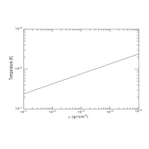
Figure 1: Temperature for which $\alpha=1$ as a function of energy density. Systems with $\alpha>1$, are above the line.

It is worth noticing that condition $\alpha>1$ can be accomplished in non very exotic systems. One of them is an interacting mixture of matter and neutrinos, which is a well-known scenario during the formation of a neutron star in a supernova explosion. In this case the heat conductivity coefficient is given by [24, 25]

$$\kappa=\frac{4}{3}bT^{3}\tau,$$ (101)

where $\tau$ is the mean collision time, $b=7N_{\nu}a/8$, $N_{\nu}$ is the number in neutrino flavors and $a$ is the radiation constant. Assuming that two viscosity coefficients vanishes, and $p\ll\rho$ then

$$\alpha=\frac{\kappa T}{\tau_{\kappa}\left(\rho+p\right)}\simeq\frac{\kappa T}{\tau\rho}.$$ (102)

Using usual units, the critical point is overtaken if

$$T>\sqrt[4]{\frac{6\rho c^{3}}{7N_{\nu}a}}\sim 4.29\times 10^{8}\rho^{1/4},$$ (103)

where we have adopted $\tau\sim\tau_{\kappa}$, $N_{\nu}=3$, $T$ is in Kelvin and $\rho$ is given in g cm${}^{-3}.$ The values of temperature, for which $\alpha=1$, are presented in figure 1 as a function of energy density. These ones are similar to the expected temperature that can be reached during hot collapse in a supernova explosion [26, $\S$ 18.6].

We would like to conclude with the following comment: for degenerate matter,when thermal conductivity is dominated by electrons, thermal relaxation time may be of the order of milliseconds (or even larger), due to larger mean free path of electrons [27] , but this is of the same order of magnitude as the time scale of the quick phase preceding neutron star formation. Therefore for this last scenario (at least) , the basic assumption of our approach is justified.

References

[1] L. Herrera, Phys. Lett. A, 165, 206,
(1992); 188, 402, (1994)
[2] A. Di Prisco, E. Fuenmayor, L. Herrera and V. Varela, Phys. Lett. A, 195, 23, (1994); A. Di Prisco, L. Herrera and V.
Varela, Gen. Rel. Gravit., (1997), (to appear)
[3] L. Herrera and V. Varela, Phys. Lett. A, 226,
143, (1997)
[4] L. Herrera et al, Class. Quantum Grav., 14,
2239, (1997)
[5] L. Herrera and J. Martínez, Class. Quantum Grav., 14, 2697,(1997)
[6] W.A. Hiscock and L. Lindblom, Ann. Phys., 151,
466, (1983)
[7] Eckart C., Phys. Rev., 58, 919, (1940)
[8] Landau L. and Lifshitz E.,Fluid Mechanics
(Pergamon Press, London), (1959)
[9] Müller I, Z. Physik, 198, 329, (1967)
[10] W. Israel and J. Stewart, Phys. Lett. A, 58,
2131, (1976); Ann. Phys. (NY), 118, 341, (1979)
[11] W.D.Arnett, Astrophys.J.218, 815, (1977)
[12] D.Kazanas, em Astrophys.J.222, L109, (1978)
[13] D.Mihalas and B.Mihalas, Foundations of Radiation
Hydrodynamics, (Oxford University Press, Oxford), (1984)
[14] H. Bondi, Proc. R. Soc. London A, 281, 39,
(1964)
[15] R.W. Lindquist, Ann. Phys. (New York), 37, 487, (1966)
[16] P.C. Vaidya, Proc. Ind. Acad. Sci. Sect. A, 33, 264, (1951)