Evolving the Bowen–York initial data for spinning black holes

Abstract

The Bowen-York initial value data typically used in numerical relativity to represent spinning black hole are not those of a constant-time slice of the Kerr spacetime. If Bowen-York initial data are used for each black hole in a collision, the emitted radiation will be partially due to the “relaxation” of the individual holes to Kerr form. We compute this radiation by treating the geometry for a single hole as a perturbation of a Schwarzschild black hole, and by using second order perturbation theory. We discuss the extent to which Bowen-York data can be expected accurately to represent Kerr holes.

I Introduction

The description of the collision of two black holes, including the total energy radiated and the waveforms to be measured by observers far from the collision region, is at this time one of the most active fields of research in general relativity. Since the latter theory has a well posed initial value problem, a good deal of effort has been devoted to finding solutions for the initial value problem, in the form of initial data sets, that may represent slices of recognizable physical processes involving black holes. One of the first examples of this kind was given by Misner [1], who derived an initial data set representing the moment of time symmetry in the head-on collision of two equal mass black holes, placed at an arbitrary distance from each other. Further developments along this line have provided a fair number of interesting initial data sets [2, 3], that can be interpreted as representing isolated but boosted and/or rotating black holes, or collisions involving two or more black holes.

Once one has the initial data, the next task is to study the evolution and the consequent emission of gravitational waves arising from the collision. Due to the complexity of the evolution equations of general relativity, numerical solutions of the full Einstein equations are available at present only for equal mass, nonspinning, holes undergoing a head-on (i.e., zero impact parameter) collision. [4, 5].

It has also been observed that for a restricted set of parameters, the evolution can be well described by treating the system as a perturbation of a single black hole [6]. This method, called the “close approximation,” has produced results that are in remarkable agreement with the full numerical results in the case where the latter are available. An appealing feature of the perturbation method is the explicit control over the parameters characterizing the perturbation. This, together with the development of some form of “error bars,” as in [7, 8], can make the method an important tool to make predictions of physical processes or to provide comparison cases to test the reliability of numerical methods.

The initial data set that is usually considered [2, 3] in the study of black hole collisions is generated using the conformal approach, in which one assumes that the spatial metric is conformally flat, and the maximal slicing condition is chosen for the extrinsic curvature. In the flat space, it is relatively simple to construct a conformally related extrinsic curvature which guarantees that the momentum constraint is solved. The Hamiltonian constraint is subsequently solved, either numerically [3] or via approximations [5, 9]. In this construction there is a series of simplifying assumptions and there is no claim that a “generic” solution has been found. It is therefore not clear that the particular solution generated is a true representation of the physical problem in which one is interested. An example of this is the Bowen and York (BY)[2] solution for a single spinning hole. It is known that this initial data set represents a dynamical situation that evolves to a Kerr black hole asymptotically in the future. Initially, however, the spacetime is not a Kerr spacetime, but can be thought (somewhat inappropriately) to differ from a Kerr solution in that it has some “gravitational wave content,” the waves that will be radiated as the spacetime evolves towards Kerr.

One can argue that this “gravitational wave content” will be radiated in a short time, and that the initial data will evolve rapidly to a stationary Kerr black hole configuration, and therefore will not greatly affect the radiation produced in a black hole collision, as long as the holes are released far from each other. The question is important enough to deserve a more careful answer. In addition, numerical relativity codes cannot be accurately run for long evolution times, so initial data will have to be specified at fairly late times, with holes fairly close together, and with the possibility that the “gravitational wave content” of the initial data is a major part of the outgoing radiation.

The purpose of this paper is to analyze the radiation from the individual holes. More specifically, we use the theory of perturbations of the Schwarzschild spacetime. We consider that we have a family of spacetimes depending on the parameter $\epsilon$, and that, in appropriate coordinate systems, metrics of the family can be expanded as

$$g_{\mu\nu}=g^{(0)}_{\mu\nu}+\epsilon h^{(1)}_{\mu\nu}+\epsilon^{2}h^{(2)}_{\mu\nu}+\cdots\ .$$ (1)

Here $g^{(0)}_{\mu\nu}$ the Schwarzschild metric, $h^{(1)}_{\mu\nu}$ is called the first order perturbation, and $h^{(2)}_{\mu\nu}$ is called the second order perturbation. To analyze the “Bowen and York spacetime,” the spacetime that evolves from Bowen and York initial data for a single spinning hole, we choose as the expansion parameter the angular momentum $J$, and we analyze both the Kerr solution and the BY spacetime to second order in $J$. The second order expansions are then compared and we find that we need only to evolve the difference between the BY spacetime and the Kerr spacetime.

The organization of this paper is as follows. In section II we give a perturbation analysis of the BY initial data. The method of evolving this initial data is described in section III. In section IV the results for radiation emitted are presented and discussed. In an Appendix we show how the Kerr metric can be written as an expansion, in angular momentum, about the Schwarzschild spacetime.

When it is useful to specify orders of expansion, and/or multipole indices, we shall use a leading subscript to denote the multipole index $\ell$, and a superscript, in parenthesis, to the right of a perturbation variable, to indicate order in $J$. The quantity ${}_{0}\psi^{(2)}$, for example, is a monopole perturbation, second order in $J$.

II The Bowen–York single rotating black hole

The Bowen–York [2] construction of initial data assumes that space-time contains a (constant $t$) slice, where the 3-metric can be written in the form $g_{ij}=\psi^{4}f_{ij}$, where $f_{ij}$ is the metric for the flat background $ds^{2}=dR^{2}+R^{2}(d\theta^{2}+\sin^{2}{\theta}\,d\phi^{2})$, while the extrinsic curvature is given by $K_{ij}=\psi^{-2}\widehat{K}_{ij}$, and satisfies $K^{i}_{i}=0$. With these assumptions the initial value constraint equations take the form

$$\widehat{K}^{ij}_{\ \ |j}=0,$$ (2)

and

$$\nabla^{2}\psi=-{1\over 8}\widehat{K}_{ij}\widehat{K}^{ij}\psi^{-7},$$ (3)

where the Laplacian, and the covariant differentiation (denoted by a vertical bar) are taken with respect to the flat space metric. The problem is not fully specified until appropriate boundary conditions are imposed on $\psi$. The Bowen–York prescription for a single black hole is that, given a certain constant $a$, Eq. (3) holds for $R\geq a$, and

$${\partial\psi\over\partial R}+{1\over 2R}\psi=0\;\;\mbox{for}\;\;R=a,$$ (4)

and

$$\psi>0\;\;,\;\;\lim_{R\rightarrow\infty}\psi=1.$$ (5)

The particular solution we are interested in corresponds to [2]

$$\widehat{\bf{K}}={3\over R^{3}}\left[(\bf{J}\wedge\bf{R})\otimes\bf{R}+\bf{R}\otimes(\bf{J}\wedge\bf{R})\right],$$ (6)

where $\bf{R}$ is the “position” vector in the flat space background, and $\bf{J}$ is a vector constant. Without loss of generality, we choose ${\bf J}=J{\bf k}$, where ${\bf k}$ is a unit vector pointing along (the positive direction of) the polar axis of the $R,\theta,\phi$ coordinate system. With this choice, the only nonvanishing components of $\widehat{\bf{K}}$ are

$$\widehat{K}_{R\phi}=\widehat{K}_{\phi R}={3J\over R^{2}}\sin^{2}{\theta}\ ,$$ (7)

We then find

$$\widehat{K}_{ij}\widehat{K}^{ij}=18{J^{2}\over R^{6}}\sin^{2}{\theta}\ .$$ (8)

We now need to solve Eq. (3). For general values of $J$, this can only be done numerically. However, we are really interested in solutions near $J=0$ (“slow rotation”) and an expansion in powers of $J$ is appropriate. The zeroth order equation is

$$\nabla^{2}\psi=0\ ,$$ (9)

and the solution that satisfies the boundary conditions is

$$\psi^{(0)}=1+a/R\ .$$ (10)

The lowest order correction to $\psi$ may now be constructed by linearizing $\psi$ about $\psi^{(0)}$ in Eq. (3). If we formally write

$$\psi=\psi^{(0)}+J^{2}\psi^{(2)}+\dots\ ,$$ (11)

the resulting equation is

$$\nabla^{2}\psi^{(2)}=-{9\over 4R^{6}}\sin^{2}{\theta}\left(1+{a\over R}\right)^{-7}\ ,$$ (12)

and the $\sin^{2}{\theta}$ factor may be expanded in Legendre polynomials, as $2[P_{0}(\cos\theta)-P_{2}(\cos\theta)]/3$.

We next write $\psi^{(2)}(R,\theta)$ as

$$\psi^{(2)}(R,\theta)=\ _{0}\psi^{(2)}(R)\,P_{0}(\cos{\theta})+\ _{2}\psi^{(2)}(R)\ P_{2}(\cos{\theta})$$ (13)

and we find that ${}_{0}\psi^{(2)}(R)$ and ${}_{2}\psi^{(2)}(R)$ satisfy the equations

$${d^{2}\left[{}_{0}\psi^{(2)}\right]\over dR^{2}}+{2\over R}{d\left[{}_{0}\psi^{(2)}\right]\over dR}=-{3\over 2R^{6}}\left(1+{a\over R}\right)^{-7}\ ,$$ (14)

and

$${d^{2}\left[{}_{2}\psi^{(2)}\right]\over dR^{2}}+{2\over R}{d\left[{}_{2}\psi^{(2)}\right]\over dR}-{6\over R^{2}}\ _{2}\psi^{(2)}={3\over 2R^{6}}\left(1+{a\over R}\right)^{-7}\ .$$ (15)

The solutions of these equations, satisfying the boundary conditions are

$$_{0}\psi^{(2)}={a^{4}+R^{4}+5aR(R+a)^{2}\over 40a^{3}(R+a)^{5}}$$ (16)

and

$${}_{2}\psi^{(2)}=-{R^{2}\over 20a(R+a)^{5}}\ .$$ (17)

With Eq. (16) we see that the conformal factor has the form

$$\psi=1+\frac{a}{R}+\frac{J^{2}}{40a^{3}}\,\frac{1}{R}+{\cal O}(1/R^{2})+{\cal O}(J^{3})\ .$$ (18)

But by the definition of the ADM mass (see for instance [2]), $\psi=1+M_{\rm ADM}/(2R)+{\cal O}(1/R^{2})$, and hence the ADM mass, to second order in $J$, is

$$M_{\rm ADM}=2a+\frac{J^{2}}{20a^{3}}\ .$$ (19)

This dependence of $M_{\rm ADM}$ on $J$, for constant $a$, is plotted in Fig. 1 as the dashed curve. Two other computations of $M_{\rm ADM}$ are also plotted, based on the integral [2, 10],

$$M_{ADM}={1\over 32\pi}\int_{r\geq a}{\hat{K}^{ij}\hat{K}_{ij}\over\psi^{7}}dv+{a\over 2}\int_{0}^{\pi}\psi\sin\theta d\theta\ .$$ (20)

The solid curve shows the result of substituting $\psi$, to second order in $J$, into the integrals in Eq. (20). The result agrees with Eq. (19) to second order in $J$, but is significantly smaller for large $J$. (The difference is due to terms higher order in $J$; the expressions are identical up to second order). The dark points show the result of a multigrid numerical code we wrote to solve the fully nonlinear initial value problem of general relativity with axisymmetry, similar to that used by Choptuik and Unruh [10].

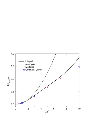
FIG. 1.: Comparison of approximate solutions to the initial value problem with a full numerical integration performed with a multigrid method. Our code uses a square grid in compactified coordinates $\rho=R/(a+R)$, $\theta$ with $200\times 200$ grid points. It achieves an accuracy similar to the test runs of Choptuik and Unruh[10]. The figure at the left compares the ADM mass of approximate and numerical solutions. The two approximations are described in the text. The figure on the right shows the percentile difference between the full numerical solution for $\psi$ and the second order approximation, for $J/a^{2}=4$, as a function of $\rho,\theta$. We see that the approximation works very well.

The results presented to this point are formally expansions to second order in the dimensionless parameter $J/a^{2}$, but $a$ itself is not a physical parameter, so the physical meaning of this expansion is unclear. For that reason we now convert our result to an expansion in the parameter $J/M^{2}$. (Here, and in subsequent expressions, we drop the “ADM” subscript on $M$. The symbol $M$ will always represent the ADM mass.) We then consider in the expressions we gave for the conformal factor,

$$\psi=1+\frac{a}{R}+J^{2}\left({}_{0}\psi^{2}+\ _{2}\psi_{2}^{2}\,P_{2}(\cos{\theta})\right)\ ,$$ (21)

that the parameter $a$ is really given by $a(M,J)$. One can obtain explicit formulas for this by considering the expression for $a(M,J)$ obtained by inverting the approximate expression Eq. (19). Alternatively, one can keep the implicit dependence of $a$ on $J$, and can replace it in the last step of a calculation, using tabulated values for $a(M,J)$ obtained from the multigrid numerical code. In this case the “second order part” is the part of $\psi$ that remains after the part zeroth order in $J/M^{2}$ is subtracted.

If the relation of $a$ and $J$ is taken from Eq. (19), the explicit formulas (correct to second order) are,

$$\psi=\Psi^{(0)}+(J/M^{2})^{2}\Psi^{(2)}=\Psi^{(0)}+(J/M^{2})^{2}\left({}_{0}\Psi^{(2)}+\ _{2}\Psi^{(2)}\,P_{2}(\cos\theta)\right)\ ,$$ (22)

with

$$\Psi^{(0)}=1+M/2R$$ (23)

$${}_{0}\Psi^{(2)}=\frac{M}{R}\frac{1+(5M/2R))(1+M/2R)^{2}+(M/2R)^{4}-(1+M/2R)^{5}}{5(1+M/2R)^{5}}$$ (24)

$${}_{2}\Psi^{(2)}=-\frac{(M/R)^{3}}{10(1+M/2R)^{5}}\ .$$ (25)

To obtain the background metric in the usual Schwarzschild form we introduce the radial coordinate $r$ with

$$R=\left(r-M+\sqrt{r^{2}-2Mr}\right)/2\ .$$ (26)

Since the conformal factor, up to second order, can be written as

$$\psi^{4}=\left(\Psi^{(0)}\right)^{4}\left[1+4\left(\frac{J}{M^{2}}\right)^{2}{\Psi^{(2)}\over\Psi^{(0)}}\right]\ ,$$ (27)

the 3-geometry to second order is given by

$$\left(1-{2M\over r}\right)g_{rr}=\frac{g_{\theta\theta}}{r^{2}}=\frac{g_{\phi\phi}}{r^{2}\sin^{2}\theta}=\left[1+4\left(\frac{J}{M^{2}}\right)^{2}{\Psi^{(2)}\over\Psi^{(0)}}\right]\ ,$$ (28)

and, in terms of the $r$ variable, we may write

$${{}_{2}\Psi^{(2)}\over\Psi^{(0)}}=-{M^{3}\over 10r^{3}}\ .$$ (29)

III Perturbative evolution of the Bowen–York initial data

We adopt the notation of Regge and Wheeler[11] for the separation into parities and the multipole decomposition of the perturbations. Because we are considering axisymmetric situations, all multipole decompositions are given in terms of Legendre polynomials $P_{\ell}(\cos\theta)$. On the initial constant-$t$ hypersurface of the BY spacetime, we can read off the perturbations of the 3-geometry from Eq. (28). The perturbations are purely second order even parity, and in the Regge-Wheeler notation, are:

$$_{2}H_{2}^{BY}=_{2}K^{BY}=4(J/M^{2})^{2}\ _{2}\Psi^{(2)}/\Psi^{(0)}=-4J^{2}/(10Mr^{3})\ ,\;\;\;\;\;\;\;\;\;G^{BY}=h_{1}^{BY}=0\ .$$ (30)

The first order perturbations contained in the BY spacetime are those specified by the extrinsic curvature in Eq. (7), which can be reexpressed as

$$K_{r\phi}=\psi^{-2}\widehat{K}_{r\phi}=\psi^{-2}\left(\frac{dR}{dr}\right)\widehat{K}_{R\phi}={3J\over r^{2}\sqrt{1-2M/r}}\sin^{2}{\theta}\ ,$$ (31)

and is identical to the extrinsic curvature given in Eq. (58) for the Kerr geoemtry. The explicit form of the metric perturbations, to first order in $J$, depends on the gauge (first order coordinate fixing) we choose. Let us choose the coordinates to first order so that the initial BY metric is the same as the first order Kerr metric given by Eq. (53) of the Appendix. That is, let us choose

$$g^{BY}_{t\phi}=2{J\over r}\sin{\theta}{\partial\over\partial\theta}P_{1}$$ (32)

to be the only nonvanishing first order initial perturbation. Since this perturbation is purely $\ell=1$, the Einstein equations require that there be no gauge independent time variation in this perturbation. Let us choose, therefore, to have the perturbation in Eq. (32) be the first order perturbation for all time. This is equivalent to the statement that we are choosing coordinates, to first order in $J$, so that the BY and the Kerr spacetimes agree, at all times, to first order in $J$.

In principle, the radiation in the BY spacetime would be found from the quadrupolar part of Einstein’s equations to second order in $J/M^{2}$. These equations contain terms linear in the $\ell=2$ second order metric perturbations, and quadratic in the first order perturbations. The general structure of these equations is discussed in Ref. [7]. In that reference it is shown how these second order equations can be combined into an equation like that of Zerilli[12, 13] for first order equations. The second order equivalent of the Zerilli equation differs only in that it has “source” terms quadratic in the first order perturbations. Since we know the first order perturbations, for all time, for the BY spacetime, we know the source term. The wave equation can therefore be solved numerically and the radiation signal found from the solution for the wave variable at large radius.

In practice, this computation can be made much simpler. Since the first order perturbations in the BY and the Kerr spacetimes are identical, the source terms will be identical in the second order Einstein equations for BY and for Kerr. We can exploit this, by evolving only the difference between the second order BY and Kerr perturbations, following the technique used by Cunningham et al.[14]. To do this, we take as our second order $\ell=2$ variable the Moncrief[15] wave variable

$$_{2}\chi_{M}(r,t)={(2r-4rM)\over(2r+3M)}\left(-2r^{2}{\partial[\,_{2}K^{(2)}]\over\partial r}+6r^{2}{\partial[\,_{2}G^{(2)}]\over\partial}r+2r\,_{2}H^{(2)}_{2}-12\,_{2}h^{(2)}_{1}\right)+4r\,_{2}K^{(2)}$$ (33)

in which ${}_{2}K^{(2)},\ _{2}G^{(2)},\ _{2}h^{(2)}_{1}$ and ${}_{2}H^{(2)}_{2}$ are second order $\ell=2$ perturbations. This Moncrief wave variable has two very useful features. First, ${}_{2}\chi_{\rm M}$ is constructed only from perturbations in the 3-geometry on the initial hypersurfaces. Second, it is invariant under second order coordinate transformations, that is, under transformations of form $(x^{\mu})^{New}=(x^{\mu})^{Old}+\xi^{\mu}$, in which $\xi^{\mu}$ is second order.

We are using here the same normalization for our wave function as in Ref. [7]. This normalization is formally the same as that of Zerilli[12], except that we expand in $P_{\ell}$ rather than $Y_{\ell m}$; as a result our ${}_{2}\chi_{M}$ is related to the variable $\widehat{K}_{2M}$ of Zerilli[12] by ${}_{2}\chi_{M}=\sqrt{5/4\pi}\widehat{K}_{2M}$. For a discussion of the relationship of the Moncrief and Zerilli variables, and various normalizations, see Ref. [16]. It is straightforward to generalize the analysis to arbitrary $\ell>2$.

We use the Moncrief wave functions ${}_{2}\chi_{\rm M}^{BY}$ to describe the Bowen York spacetime, and ${}_{2}\chi_{\rm M}^{\rm Kerr}$ for Kerr. The initial value for ${}_{2}\chi_{\rm M}^{\rm BY}$ are taken from Eq. (30) and the value of ${}_{2}\chi_{\rm M}^{\rm Kerr}$, initially and for all time, are taken from the expansion in the Appendix, from which we have,

$${}_{2}{H}^{\rm Kerr}_{0} = -{4J^{2}\over 3Mr^{2}(r-2M)},$$ (34)

$${}_{2}{H}^{\rm Kerr}_{1} = 0$$ (35)

$${}_{2}{H}^{\rm Kerr}_{2} = {2J^{2}\over 3M^{2}r^{2}}$$ (36)

$${}_{2}{K}^{\rm Kerr} = -{2J^{2}(4M+r)\over 3M^{2}r^{3}}$$ (37)

$${}_{2}{G}^{\rm Kerr} = -{J^{2}(2M+r)\over 3M^{2}r^{3}}\ .$$ (38)

We now define a “radiative” Moncrief wave function by

$${}_{2}\chi^{\rm rad}\equiv\ _{2}\chi_{\rm M}^{BY}-\ _{2}\chi_{\rm M}^{\rm Kerr}\ .$$ (39)

Since the first order perturbations, and therefore the source terms, for ${}_{2}\chi_{\rm M}^{BY}$ and for ${}_{2}\chi_{\rm M}^{\rm Kerr}$ are the same, ${}_{2}\chi^{\rm rad}$ satisfies a homogeneous Zerilli function

$${\partial^{2}\left[{}_{2}\chi^{\rm rad}(t,r)\right]\over\partial{r^{*}}^{2}}-{\partial^{2}\left[{}_{2}\chi^{\rm rad}(t,r)\right]\over\partial t^{2}}-V(r^{*})\ _{2}\chi^{\rm rad}(t,r)=0\ ,$$ (40)

where

$$r^{*}\equiv r+2M\ln[r/(2M)-1]\ ,$$ (41)

and where $V$ is the $\ell=2$ Zerilli potential

$$V(r)=6\left(1-2{M\over r}\right){4r^{3}+4r^{2}M+6rM^{2}+3M^{3}\over r^{3}(2r+3M)^{2}}\ .$$ (42)

A word of explanation is appropriate about the properties of ${}_{2}\chi_{\rm M}$ under a coordinate transformation. As already stated, ${}_{2}\chi_{\rm M}$ is invariant under a transformation in which the coordinates change only to second order. This is why we can use Eqs. (34) – (38) to evaluate ${}_{2}\chi_{\rm M}^{\rm Kerr}$, and Eq. (30) for ${}_{2}\chi_{\rm M}^{BY}$, though the second order metric perturbations used are clearly in different gauges. The point is that we know that the second order perturbations can be brought into the same second order gauge with second order gauge transformations, and that this has no effect on ${}_{2}\chi_{\rm M}^{\rm Kerr}$ or on ${}_{2}\chi_{\rm M}^{BY}$, and hence no effect on ${}_{2}\chi^{\rm rad}$. It should be realized that ${}_{2}\chi_{\rm M}$ is not invariant under a first order change of coordinates. If we were to perform, say, a first order change in the coordinates used in the Appendix, then the value of ${}_{2}\chi_{\rm M}^{\rm Kerr}$ we would compute would change. It is important, therefore, that no first order change in coordinates is needed for the Kerr expansion in the Appendix, or the BY spacetime in Sec. II. They are already in the same first order gauge.

The initial ${}_{2}\chi_{\rm M}$ for this equation is simply the known difference between the initial forms of ${}_{2}\chi_{\rm M}^{BY}$ and ${}_{2}\chi_{\rm M}^{\rm Kerr}$, and turns out to be

$$_{2}\chi^{\rm rad}|_{t=0}=\frac{2J^{2}}{5M^{2}r^{3}}\ \left(\frac{-5r^{3}-7Mr^{2}+25M^{2}r+60M^{3}}{2r+3M}\right)\ .$$ (43)

There are no second order perturbations to the extrinsic curvature of a constant time slice of Kerr, or in the BY initial data. The first of these conclusions follows from an explicit computation based on the metric in the Appendix. One finds that the extrinsic curvature contains only odd powers of $J$. (This conforms to the intuition that suggests that reversing the direction of $J$ should reverse the sign of extrinsic curvature.) The conformally related extrinsic curvature $\widehat{K}_{ij}$ for the BY initial data is given to all orders by Eq. (6). The second order perturbations in the conformal factor mean that the extrinsic curvature $\widehat{K}_{ij}=\psi^{-2}\widehat{K}_{ij}$ will contain perturbations of odd orders in $J$, due to the perturbations of even order contained in $\psi$. Since there are no second order contributions to the extrinsic curvature, of either BY or Kerr, it follows that

$$\left.\frac{d}{dt}\left({}_{2}\chi^{\rm rad}\right)\right|_{t=0}=0\ .$$ (44)

The wave equation of Eqs. (40) – (42), with the cauchy data of Eqs. (43) – (44), is simply solved numerically for ${}_{2}\chi^{\rm rad}(t,r)$, and from the solution we can find

$${}_{2}\chi_{\rm M}^{BY}(t,r)=\ _{2}\chi^{\rm rad}(t,r)+\ _{2}\chi_{\rm M}^{\rm Kerr}(r)\ ,$$ (45)

where ${}_{2}\chi_{\rm M}^{\rm Kerr}(r)$ is the known, time independent, Kerr solution. The radiative power (see Ref. [7]) contained in the BY spacetime is then given by

$${\rm Power}=\frac{3}{10}\left(\frac{d}{dt}_{2}\chi_{\rm M}^{BY}\right)^{2}=\frac{3}{10}\left(\frac{d}{dt}_{2}\chi^{\rm rad}\right)^{2}\ ,$$ (46)

and this is the gravitational radiation power emitted as the BY solution settles into its Kerr final form. The energy radiated is the time integral of this expression.

FIG. 2.: The radiated waveform for a single spinning Bowen and York black hole, computed treating the spacetime as a perturbation of Schwarzschild. The waveform, extracted at $r=20M$, is dominated by quasinormal ringing which persists long enough to contaminate radiation coming out from a head on collision of black holes. We display the waveforms corresponding to the different choices of background mass used in perturbation theory. The significant differences among these curves illustrates the importance of the choice of the background mass in perturbative calculations, i.e., on the way in which the ADM mass $M$ is taken to depend on $J$, for a given value of $a$. The bold curve uses the “correct” ADM mass computed numerically with the multigrid code. The thin curve was computed with expression $M=2a+J^{2}/(20a^{3})$ (see text) which is correct to second order in $J$. The dashed curve uses $M=2a$, and ignores the influence of $J$ on $M$, for given $a$. Previous experience with perturbation calculations for which numerical relativity comparisons were available strongly suggests that the curve with the numerically computed ADM mass is the most accurate.

IV Results and discussion

In Fig. 2 we show the radiated waveform, as a function of $t$, for fixed, large $r$, from which we may infer the effective time for the decay of the Bowen–York rotating black hole into its final Kerr state. It is clear that the wave form is dominated by quasinormal ringing. This means that the “initial burst” of energy generated as the hole relaxes to Kerr form can contaminate the evolution for some time.

FIG. 3.: The total radiated energy computed for “BY relaxation.” The method is formally correct only to lowest (fourth) order in the expansion parameter $J/M_{ADM}^{2}$. For a description of the various ADM masses involved, see the caption of figure 2.

In Fig. 3 we show the total energy radiated as a function of $J/M^{2}$. Whatever choice we make for the $J$ dependence of the ADM mass, our perturbation calculation for $\chi^{\rm rad}$ is formally correct only to second order in $J/M^{2}$. Since the radiated energy is quadratic in $\chi^{\rm rad}$, the energy results displayed in Fig. 3 are formally correct only to fourth order in $J/M^{2}$, the lowest nontrivial order. The results in Fig. 3, cannot therefore be trusted for $J/M^{2}$ near the astrophysically interesting limit $J/M^{2}\approx 1$. We suspect that the curve corresponding to the numerical ADM mass is reliable within a factor of two or so up to $J/M^{2}=0.8$. A more accurate evaluation will require either fully nonlinear numerical relativity, or a calculation using second order perturbations around the Kerr solution.

According to Fig. 3, the “BY relaxation energy,” the energy emitted as a single BY hole relaxes to a Kerr hole appears to be small. It should be kept in mind, however, that the total radiation in a black hole coalescence can be comparably small. For a head on collision of nonspinning holes the total radiated energy is of order $10^{-3}$ of the total ADM mass. Head on collisions, of course, are not of primary astrophysical interest. For the “merger” phase of equal mass holes, radiated energy is expected to be several percent[17]. In this case, the BY relaxation energy would be negligibly small. It would, furthermore, be emitted within a few quasinormal periods of a single hole, while the merger and ringdown of the final hole formed would require a time an order of magnitude longer.

V Acknowledgments

We were able to write our multigrid code by studying a code of the NCSA/Potsdam group. We wish to thank Peter Anninos for help with this. Using the ADM mass instead of the $a$ parameter was an idea that arose in various discussions that initially involved John Baker and Steve Brandt. This work was supported in part by grants NSF-INT-9512894, NSF-PHY-9423950, NSF-PHY-9507719, by funds of the University of Córdoba, the University of Utah, the Pennsylvania State University and its Office for Minority Faculty Development, and the Eberly Family Research Fund at Penn State. We also acknowledge support of CONICET and CONICOR (Argentina). JP also acknowledges support from the Alfred P. Sloan Foundation through an Alfred P. Sloan fellowship.

Appendix: The Kerr metric as a perturbation of a Schwarzschild black hole

The Kerr metric in Boyer - Lindquist coordinates takes the form

$$ds^{2} = {\Delta-(J/M)^{2}\sin^{2}{\theta}\over\Sigma}dt^{2}-2(J/M)\sin^{2}{\theta}{\rho^{2}+(J/M)^{2}-\Delta\over\Sigma}dtd\phi$$ (48)

$$+{(\rho^{2}+(J/M)^{2})^{2}-\Delta(J/M)^{2}\sin^{2}{\theta}\over\Sigma}\sin^{2}{\theta}d\phi^{2}+{\Sigma\over\Delta}d\rho^{2}+\Sigma d\theta^{2}$$

where $\Sigma=\rho^{2}+(J/M)^{2}\cos^{2}{\theta}$ and, $\Delta=\rho^{2}+(J/M)^{2}-2M\rho$.

If we assume $J<M^{2}$, (48) is defined only for $\rho>M+\sqrt{M^{2}-(J/M)^{2}}$, since $\Delta=0$ for $\rho=M+\sqrt{M^{2}-(J/M)^{2}}$.

The metric (48) reduces to the Schwarzschild metric, in the range $\rho>2M$, for $J=0$. It seems reasonable, therefore, to try to find an expansion of (48), in powers of $J$, as a perturbation of a Schwarzschild black hole. This expansion, however, would fail near $\rho=2M$, because the metric coefficient $g_{\rho\rho}$ does not have the required analyticity properties. To avoid this problem we introduce a new coordinate $r$, such that

$$r^{2}-2Mr=\rho^{2}+(J/M)^{2}-2M\rho$$ (49)

With this definition we have that $\Delta=0$ corresponds to $r=2M$. We may invert (49) to

$$\rho=M+\sqrt{(r-M)^{2}-(J/M)^{2}}$$ (50)

Then, for $r>2M$, and $J<M^{2}$, the right hand side may be expanded in powers of $J$. The leading terms are

$$\rho=r-{J^{2}\over 2M^{2}(r-M)}\ .$$ (51)

In fact, one can easily check that all the metric coefficients admit a convergent power series expansion in $J$. To leading order we have

$$g_{tt} = \left(1-{2M\over r}\right)\left(-1+{J^{2}(r+2M)\over 3Mr^{2}(r-M)(r-2M)}P_{0}-{4J^{2}\over 3Mr^{2}(r-2M)}P_{2}+{\cal{O}}([J/M^{2}]^{4})\right)$$ (52)

$$g_{t\phi} = 2{J\over r}\sin{\theta}{\partial\over\partial\theta}P_{1}+{\cal{O}}([J/M^{2}]^{3})$$ (53)

$$g_{rr} = \left(1-{2M\over r}\right)^{-1}\left(1+{J^{2}(Mr+r^{2}+M^{2})\over 3M^{2}r^{2}(r-M)^{2}}P_{0}+{2J^{2}\over 3M^{2}r^{2}}P_{2}+{\cal{O}}([J/M^{2}]^{4})\right)$$ (54)

$$g_{\theta\theta} = r^{2}\left[1-{J^{2}(2M^{2}+r^{2})\over 3M^{2}r^{3}(r-M)}P_{0}-{2J^{2}(4M+r)\over 3M^{2}r^{3}}P_{2}-{J^{2}(r+2M)\over 3M^{2}r^{3}}{\partial^{2}\over\partial\theta^{2}}P_{2}+{\cal{O}}([J/M^{2}]^{4})\right]$$ (55)

$$g_{\phi\phi} = r^{2}\sin^{2}{\theta}\left[1-{J^{2}(2M^{2}+r^{2})\over 3M^{2}r^{3}(r-M)}P_{0}-{2J^{2}(4M+r)\over 3M^{2}r^{3}}P_{2}\right.$$ (57)

$$\left.-{J^{2}(r+2M)\over 3M^{2}r^{3}}\cot{\theta}{\partial\over\partial\theta}P_{2}+{\cal{O}}([J/M^{2}]^{4})\right]\ ,$$

where $P_{0}=1$, $P_{1}=\cos{\theta}$ and, $P_{2}=(3/2)\cos^{2}{\theta}-1/2$ are Legendre polynomials.

From this metric it is straightforward to compute, to first order in $J$, the extrinsic curvature of a $t=$ constant surface. If we let $\vec{n}$ be the future directed normal to a $t=$  constant hypersurface, then, the extrinsic curvature is $K_{ij}=-n_{i|j}$, where the bar denotes covariant differentiation with respect to the 3-geometry. The normal has only a single covariant component $n_{t}$ which, to first order in $J$, is $n_{t}=-1/\sqrt{1-2M/r}$. With this, a straightforward computation shows that the only nonvanishing first order components of $K_{ij}$ are

$$K_{r\phi}=K_{\phi r}=\frac{3J}{r^{2}\sqrt{1-2M/r}}\sin^{2}\theta\ .$$ (58)

REFERENCES

- [1] C. Misner, Phys. Rev. D118, 1110 (1960).
- [2] J. Bowen, J. York, Phys. Rev. D21, 2047 (1980).
- [3] G. B. Cook, M. W. Choptuik, M. R. Dubal , Phys. Rev. D 47, 1471 (1993); G. B. Cook, Phys. Rev. D 50, 5025 (1994); Ph.D. thesis, University of North Carolina at Chapel Hill, Chapel Hill, North Carolina, 1990.
- [4] P. Anninos, D. Hobill, E. Seidel, L. Smarr, W.-M. Suen, Phys. Rev. Lett. 71, 2851 (1993); Phys. Rev. D 52, 2044 (1995).
- [5] J. Baker, A. Abrahams, P. Anninos, S. Brandt, R. Price, J. Pullin, E. Seidel, Phys. Rev. D55, 829 (1997).
- [6] R. Price, J. Pullin, Phys. Rev. Lett. 72, 3297 (1994).
- [7] R. Gleiser, O. Nicasio, R. Price, J. Pullin, Class. Quan. Grav. 13, L117 (1996).
- [8] R. Gleiser, O. Nicasio, R. Price, J. Pullin, Phys. Rev. Lett. 77, 4483 (1996).
- [9] J. Pullin, Fields Inst. Commun. 15, 117 (1997).
- [10] M. Choptuik, W. Unruh, Gen. Rel. Grav. 18, 813 (1986).
- [11] T. Regge, J. Wheeler, Phys. Rev. 108, 1063 (1957).
- [12] F. J. Zerilli, Phys. Rev. Lett. 24 737 (1970).
- [13] F. J. Zerilli, Phys. Rev. D2 2141 (1970).
- [14] C. Cunningham, R. Price, V. Moncrief, Astroph. J. 236, 674 (1980).
- [15] V. Moncrief, Ann. Phys. (NY) 88, 323 (1974).
- [16] C.O. Lousto and R.H. Price, Phys. Rev. D55, 2124 (1997).
- [17] É.É. Flanagan and S.A. Hughes, preprint gr-qc 9701039.