Scalar Field Quantum Inequalities in Static Spacetimes

Abstract

We discuss quantum inequalities for minimally coupled scalar fields in static spacetimes. These are inequalities which place limits on the magnitude and duration of negative energy densities. We derive a general expression for the quantum inequality for a static observer in terms of a Euclidean two-point function. In a short sampling time limit, the quantum inequality can be written as the flat space form plus subdominant correction terms dependent upon the geometric properties of the spacetime. This supports the use of flat space quantum inequalities to constrain negative energy effects in curved spacetime. Using the exact Euclidean two-point function method, we develop the quantum inequalities for perfectly reflecting planar mirrors in flat spacetime. We then look at the quantum inequalities in static de Sitter spacetime, Rindler spacetime and two- and four-dimensional black holes. In the case of a four-dimensional Schwarzschild black hole, explicit forms of the inequality are found for static observers near the horizon and at large distances. It is show that there is a quantum averaged weak energy condition (QAWEC), which states that the energy density averaged over the entire worldline of a static observer is bounded below by the vacuum energy of the spacetime. In particular, for an observer at a fixed radial distance away from a black hole, the QAWEC says that the averaged energy density can never be less than the Boulware vacuum energy density.

I Introduction

In a recent paper [1], we derived a general form of the quantum inequality (QI) for quantized scalar fields in static curved spacetimes. The quantum inequalities are uncertainty type relations which constrain the magnitude and duration of negative energy that may be present in a spacetime. This was an extension of the previous work carried out by Ford and Roman [2, 3, 4, 5] which dealt with the quantum inequalities for scalar fields in two- and four-dimensional Minkowski spacetime. In curved spacetimes, it was found that the quantum inequality could be written in terms of a sum of mode functions for the scalar field. With the general form of the quantum inequality in hand, we then proceeded to look at the static cases of the three-dimensional closed universe and the four-dimensional Robertson-Walker spacetimes. Exact functional forms for the quantum inequalities were developed in these spacetimes. It was found that the curved space quantum inequalities could be written as the flat space quantum inequalities multiplied by a “scale” function which detailed the behavior of the inequalities at various ratios of the sampling time to the radius of curvature of the spacetime. In the long sampling time limit, the quantum inequality was substantially modified by the scale function. However, in the short sampling time limit, the scale functions tend to 1, yielding the flat space quantum inequality. This behavior had first been predicted to exist by Ford and Roman in a paper dealing with negative energy around wormholes [6]. It was argued that by making the sampling time of the quantum inequality much shorter than a minimum characteristic curvature scale, then the spacetime could be considered locally flat and the Minkowski space quantum inequality should hold. This method has since been applied to the Alcubierre “Warp Drive” metric [7, 8] to show that the negative energy that makes up the walls of the warp bubble has to be constrained to exceptionally thin walls, usually on the order of hundreds, or perhaps thousands of Planck lengths at most. Similar results were found for the Krasnikov metric [9, 10], where the negative energy that is needed must also be confined to exceptionally thin walls.

In our earlier work [1], the quantum inequality was derived for stationary observers in static spactimes where the magnitude of the $g_{tt}$ component of the metric was 1. In this paper we will extend the derivation of the quantum inequalities to the entire class of static spacetime metrics of the form

$${ds}^{2}=-|g_{tt}({\bf x})|{dt}^{2}+g_{ij}({\bf x})dx^{i}dx^{j}\;.$$ (1)

In Sec. II we will derive the general form of the quantum inequality for static observers in such spacetimes, and show that it may be written in terms of a Euclidean Green’s (two-point) function. We will show in Sec. III that in the infinite sampling time limit the quantum inequality reduces to the “quantum averaged weak energy condition” (QAWEC) which can be written in the form

$$\int_{-\infty}^{\infty}\left(\langle\psi|T_{00}/|g_{tt}|\,|\psi\rangle-\rho_{vac}\right)d\tau\geq 0\,.$$ (2)

The quantum averaged weak energy condition says that along the entire world-line of a static observer, the sampled energy density can never be more negative than the vacuum energy, $\rho_{vac}$. Here the vacuum energy is obtained using the timelike killing vector to define positive frequency.

In Sec. IV we will perform a short time expansion of the two-point function. It is found that the leading term of the expansion of the curved space quantum inequality is indeed of the flat space form. In addition, the first two corrections to the leading order term will be explored. We will show that they depend only on the geometric properties of the spacetime such as the metric, scalar curvature, etc.

In Sec. V we will look at the exact form of the quantum inequality developed for a half infinite flat spacetime. We will see that the presence of a perfectly reflecting, infinite planar mirror modifies the flat space quantum inequality. In addition we will look at the case of the quantum inequality between two parallel mirrors. Both of these cases will be developed by first determining the Feynman Green’s function by the method of images, and then using the formalism developed in Sec. II to find the respective quantum inequalities.

Finally, we will look at the quantum inequalities in spacetimes in which there exist horizons. We will begin with the two-dimensional Rindler coordinates and then move on to the static coordinate representation of de Sitter spacetime. Finally in Sec. VII we will look at the case of two- and four-dimensional black holes. In two-dimensions, we will find the exact form of the quantum inequality for static observers sitting at fixed radii outside of the black hole. In the case of the four dimensional black hole, because there is no known analytic solution for the mode functions of the scalar field, we find the quantum inequality in the limits $r\rightarrow 2M$ and $r\rightarrow\infty$. In the limit of long sampling time, the QAWEC is recovered for these spacetimes.

II The Scalar Field Quantum Inequality

Because this derivation closely resembles that developed earlier [1], we will only highlight the necessary steps to replicate the proof for the metric in Eq. (1). On such a fixed background, the wave equation

$$\Box\phi-m^{2}\phi={1\over\sqrt{|g|}}\partial_{\alpha}\left(\sqrt{|g|}g^{\alpha\beta}\partial_{\beta}\phi\right)-m^{2}\phi=0$$ (3)

becomes

$$-{1\over|g_{tt}|}\partial_{t}^{2}\phi+\nabla^{j}\nabla_{j}\phi-m^{2}\phi=0,$$ (4)

where $g={\rm det}(g_{\mu\nu})$, $\nabla_{i}$ is the covariant derivative in the spacelike hypersurfaces orthogonal to the Killing vector, and $m$ is the mass of the field. Units where $\hbar=c=G=1$ are used throughout this paper. The positive frequency mode function solutions can be written as

$$f_{\lambda}({\bf x},t)=\,U_{\lambda}({\bf x})\,e^{-i\omega t},$$ (5)

where $U_{\lambda}({\bf x})$ is the solution to the Helmholtz equation

$$\nabla^{j}\nabla_{j}U_{\lambda}+(\omega^{2}_{\lambda}/|g_{tt}|-m^{2})U_{\lambda}=0\,.$$ (6)

The label $\lambda$ represents the set of quantum numbers necessary to specify the mode. Additionally, the mode functions are defined to have unit Klein-Gordon norm. A general solution of the scalar field $\phi$ can then be expanded in terms of creation and annihilation operators as

$$\phi(x)=\sum_{\lambda}{\bigl{(}a_{\lambda}f_{\lambda}+a^{\dagger}_{\lambda}f^{\ast}_{\lambda}\bigr{)}},$$ (7)

where quantization is carried out over a finite box or universe. If the spacetime has infinite spatial extent, then we replace the summation by an integral over all of the possible modes.

In the development of the quantum inequality, we will concern ourselves only with static observers, whose four-velocity, $u^{\mu}=(|g_{tt}|^{-1/2},{\bf 0})$, is parallel to the direction of the timelike Killing vector. These are geodesic observers in the case that $g_{tt}$ is a constant, but otherwise are non-geodesic. The energy density (for minimal coupling) that such an observer measures is given by

$$\rho=T_{\alpha\beta}u^{\alpha}u^{\beta}={1\over|g_{tt}|}T_{00}={1\over 2}\left[{1\over|g_{tt}|}(\partial_{t}\phi)^{2}+\nabla^{j}\phi\nabla_{j}\phi+m^{2}\phi^{2}\right]\,.$$ (8)

Upon substitution of the above mode function expansion into Eq. (8), one finds that there exists a vacuum energy term which is divergent upon summation. A regularization and renormalization scheme is needed to define the physical energy density. This may be side-stepped by concentrating attention upon the difference between the energy density in an arbitrary state and that in the vacuum state, as was done in Ref. [1, 4]. We will therefore concern ourselves primarily with the normal ordered quantity

$$:\rho:\;=\rho-\langle 0|\rho|0\rangle,$$ (9)

where $|0\rangle$ represents the Fock vacuum state defined by the global timelike Killing vector. In cases where the renormalized value of $\langle 0|\rho|0\rangle$ is known, we can convert the difference inequality into an inequality on the renormalized energy density in an arbitrary state.

The energy density as defined above is valid along the entire worldline of the observer. However, let us sample the energy density only along some finite interval of the geodesic. This may be accomplished by means of a weighting function which has a characteristic time $t_{0}$, such as the Lorentzian function,

$$h(t)={t_{0}\over\pi}\,{1\over{t^{2}+t_{0}^{2}}}.$$ (10)

The integral over all time of $h(t)$ is equal to one and the width of the Lorentzian is characterized by $t_{0}$. Using such a weighting function, one finds that the averaged energy difference is given by

$$\Delta\hat{\rho} \equiv {t_{0}\over\pi}\int_{-\infty}^{\infty}{{\langle:T_{00}/|g_{tt}|:\rangle dt}\over{t^{2}+t_{0}^{2}}}$$ (11)

$$= {\rm Re}\sum_{\lambda\lambda^{\prime}}\left\{{{\omega\omega^{\prime}}\over|g_{tt}|}\left[U_{\lambda}^{*}U_{\lambda^{\prime}}e^{-|\omega-\omega^{\prime}|t_{0}}\langle a_{\lambda}^{\dagger}a_{\lambda^{\prime}}\rangle-U_{\lambda}U_{\lambda^{\prime}}e^{-(\omega+\omega^{\prime})t_{0}}\langle a_{\lambda}a_{\lambda^{\prime}}\rangle\right]\right.$$ (14)

$$\qquad+\left[\nabla^{j}U_{\lambda}^{*}\nabla_{j}U_{\lambda^{\prime}}e^{-|\omega-\omega^{\prime}|t_{0}}\langle a_{\lambda}^{\dagger}a_{\lambda^{\prime}}\rangle+\nabla^{j}U_{\lambda}\nabla_{j}U_{\lambda^{\prime}}e^{-(\omega+\omega^{\prime})t_{0}}\langle a_{\lambda}a_{\lambda^{\prime}}\rangle\right]$$

$$\qquad+m^{2}\left.\left[U_{\lambda}^{*}U_{\lambda^{\prime}}e^{-|\omega-\omega^{\prime}|t_{0}}\langle a_{\lambda}^{\dagger}a_{\lambda^{\prime}}\rangle+U_{\lambda}U_{\lambda^{\prime}}e^{-(\omega+\omega^{\prime})t_{0}}\langle a_{\lambda}a_{\lambda^{\prime}}\rangle\right]\right\}.$$

From this point onward, the derivation continues along the lines of that in Ref. [1]. After some algebra, and application of the inequalities derived in previous papers [1, 5], one finds

$$\Delta\hat{\rho}\geq-\sum_{\lambda}\left({\omega_{\lambda}^{2}\over|g_{tt}|}+{1\over 4}\nabla^{j}\nabla_{j}\right)|U_{\lambda}({\bf x})|^{2}{\rm e}^{-2\omega_{\lambda}t_{0}}\,,$$ (15)

which can be rewritten as

$$\Delta\hat{\rho}\geq-{1\over 4}\left({\partial_{t_{0}}^{2}\over|g_{tt}|}+\nabla^{j}\nabla_{j}\right)\sum_{\lambda}|U_{\lambda}({\bf x})|^{2}{\rm e}^{-2\omega_{\lambda}t_{0}}\,.$$ (16)

There is a more compact notation in which Eq. (16) may be expressed. If we take the original metric, Eq. (1), and Euclideanize the time by allowing $t\rightarrow it_{0}$ then the Euclidean box operator is defined by

$$\Box_{E}\equiv{\partial_{t_{0}}^{2}\over|g_{tt}|}+\nabla^{j}\nabla_{j}\,.$$ (17)

In addition, the sum of the mode functions is equal to the Euclidean two-point function

$$G_{E}({\bf x},-t_{0};{\bf x},+t_{0})=\sum_{\lambda}|U_{\lambda}({\bf x})|^{2}{\rm e}^{-2\omega_{\lambda}t_{0}}$$ (18)

where the spatial separation is allowed to go to zero but the time separation is $2t_{0}$. The Euclidean two-point function is the counterpart of the Feynman Green’s function for the Lorentzian metric. The two are related by

$$G_{E}({\bf x},t;{\bf x}^{\prime},t^{\prime})=iG_{F}({\bf x},it;{\bf x}^{\prime},it^{\prime}).$$ (19)

This allows us to write the quantum inequality in any static curved spacetime as

$$\Delta\hat{\rho}\geq-{1\over 4}\Box_{E}\,G_{E}({\bf x},-t_{0};{\bf x},+t_{0}).$$ (20)

We see that once we are given a metric which admits a timelike Killing vector, we can calculate the limitations on the negative energy densities by either of two methods. If we know the solutions to the wave equation, then we may construct the inequality from the summation of the mode functions. More elegantly, if the Feynman two-point function is known in the spacetime, then we may immediately calculate the inequality by first Euclideanizing and then taking the appropriate derivatives.

III The Quantum Averaged Weak Energy Condition

Let us return to the form of the the quantum inequality given by Eq. (15),

$$\Delta\hat{\rho}\geq-\sum_{\lambda}\left({\omega_{\lambda}^{2}\over|g_{tt}|}+{1\over 4}\nabla^{j}\nabla_{j}\right)|U_{\lambda}({\bf x})|^{2}{\rm e}^{-2\omega_{\lambda}t_{0}}\,.$$ (21)

Since we are working in static spacetimes, the vacuum energy does not evolve with time, so we can rewrite this equation simply by adding the renormalized vacuum energy density $\rho_{vacuum}$ to both sides. We then have

$$\hat{\rho}_{Ren.}\geq-\sum_{\lambda}\left({\omega_{\lambda}^{2}\over|g_{tt}|}+{1\over 4}\nabla^{j}\nabla_{j}\right)|U_{\lambda}({\bf x})|^{2}{\rm e}^{-2\omega_{\lambda}t_{0}}+\rho_{vacuum}({\bf x})\,,$$ (22)

where $\hat{\rho}_{Ren.}$ is the sampled, renormalized energy density in any quantum state. Let us now take the limit of the sampling time $t_{0}\rightarrow\infty$. We find (under the assumption that there exist no modes which have $\omega_{\lambda}=0$) that

$$\lim_{t_{0}\rightarrow\infty}{t_{0}\over\pi}\int_{-\infty}^{\infty}{\langle T_{00}/|g_{tt}|\rangle_{Ren.}\over t^{2}+t_{0}^{2}}dt\geq\rho_{vacuum}({\bf x}),$$ (23)

This leads directly to the “quantum averaged weak energy condition” for static observers,

$$\int_{-\infty}^{+\infty}\left(\langle\psi|T_{00}/|g_{tt}||\psi\rangle_{Ren.}-\rho_{vacuum}\right)dt\geq 0.$$ (24)

This is a departure from the classical averaged weak energy condition,

$$\int_{-\infty}^{+\infty}\langle\psi|T_{00}/|g_{tt}|\,|\psi\rangle_{Ren.}dt\geq 0.$$ (25)

We see that the derivation of the QAWEC leads to the measured energy density along the observers geodesic being bounded below by the vacuum energy. Recently, there has been much discussion about how badly the vacuum energy violates the classical energy conditions. For example Visser looked at the specific case of the violation of classical energy conditions for the Boulware, Hartle-Hawking, and Unruh vacuum states [11, 12, 13, 14] around a black hole. However the vacuum energy is not a classical phenomenon, so it necessarily need not obey classical energy constraints. From the QAWEC we see that the sampled energy density is bounded below by the vacuum energy in the long sampling time limit.

IV Expansion of the QI for Short Sampling Times

We now consider the expansion of the two-point function for small times. We assume that the two-point function has the Hadamard form [15]

$$G(x,x^{\prime})={i\over 8\pi^{2}}\left[{\Delta^{1/2}\over\sigma+i\epsilon}+V\ln(\sigma+i\epsilon)+W\right]\,,$$ (26)

where $2\sigma(x,x^{\prime})$ is the square of the geodesic distance between the spacetime points $x$ and $x^{\prime}$,

$$\Delta\equiv-g^{-1/2}(x)\,{\rm det}(\sigma_{;ab^{\prime}})\>g^{-1/2}(x^{\prime}),$$ (27)

is the Van Vleck-Morette determinant, and $V(x,x^{\prime})$ and $W(x,x^{\prime})$ are regular biscalar functions. In general, these functions can be Taylor series expanded in powers of $\sigma$,

$$V(x,x^{\prime})=\sum_{n=0}^{\infty}V_{n}(x,x^{\prime})\sigma^{n}\,,$$ (28)

where $V_{n}$ (and $W_{n}$) is also a regular biscalar function with

$$V_{0} = v_{0}-{1\over 2}v_{0;a}\,\sigma^{a}+{1\over 2}v_{0ab}\,\sigma^{a}\sigma^{b}+{1\over 6}(-{3\over 2}v_{0ab;c}+{1\over 4}v_{0;(abc)})\sigma^{a}\sigma^{b}\sigma^{c}+\cdots,$$ (29)

$$V_{1} = v_{1}-{1\over 2}v_{1;a}\,\sigma^{a}+\cdots,$$ (30)

where $\sigma^{\nu}=\sigma^{;\nu}$. The coefficients, $v_{0}$, $v_{0ab}$, …are strictly geometrical objects given by

$$v_{0} = {1\over 2}\left[(\xi-{1\over 6})R+m^{2}\right],$$ (31)

$$v_{0ab} = -{1\over 180}R_{pqra}{R^{pqr}}_{b}-{1\over 180}R_{apbq}R^{pq}+{1\over 90}R_{ap}{R_{b}}^{p}-{1\over 120}\Box R_{ab}$$ (33)

$$+({1\over 6}\xi-{1\over 40})R_{;ab}+{1\over 12}(\xi-{1\over 6})RR_{ab}+{1\over 12}m^{2}R_{ab}\,,$$

$$v_{1} = {1\over 720}R_{pqrs}R^{pqrs}-{1\over 720}R_{pq}R^{pq}-{1\over 24}(\xi-{1\over 5})\Box R+{1\over 8}(\xi-{1\over 6})^{2}R^{2}$$ (35)

$$+{1\over 4}m^{2}(\xi-{1\over 6})R+{1\over 8}m^{4}.$$

We can then express the Green’s function as

$$G(x,x^{\prime}) = {i\over 8\pi^{2}}\left\{{1+{1\over 12}R_{ab}\sigma^{a}\sigma^{b}\ -\cdots\over\sigma+i\epsilon}+\left[(v_{0}-{1\over 2}v_{0;a}\sigma^{a}+{1\over 2}v_{0ab}\sigma^{a}\sigma^{b}\ +\cdots)\right.\right.$$ (37)

$$\qquad\left.\left.+(v_{1}-{1\over 2}v_{1;a}\sigma^{a}+\cdots)\sigma+\cdots\right]\ln(\sigma+i\epsilon)+W\right\}$$

where we have also used the Taylor series expansion of the Van Vleck-Morette determinant [15],

$$\Delta^{1/2}=1+{1\over 12}R_{ab}\sigma^{a}\sigma^{b}-{1\over 24}R_{ab;c}\sigma^{a}\sigma^{b}\sigma^{c}+\cdots\,.$$ (38)

We neglect $W$, the state dependent part of the Green’s function, because it is regular as $\sigma\rightarrow 0$. The dominant contributions to the quantum inequality come from the divergent portions of the Green’s function in the $\sigma\rightarrow 0$ limit.

Let us find the geodesic distance between two spacetime points, along a curve starting at $({\bf x}_{0},-t_{0})$ and ending at $({\bf x}_{0},+t_{0})$. For spacetimes in which $|g_{tt}|=1$, the geodesic path between these two spacetime points is a straight line. Therefore, the geodesic distance is simply $2t_{0}$. However, in a more generic static spacetime where $g_{tt}({\bf x})$ is not constant, the geodesic path between the above two spacetime points is a curve, with the observer’s spatial position changing throughout time. Thus, we must now solve the equations of motion for the observer. In terms of an affine parameter $\lambda$, the geodesic equations are found to be

$${dt\over d\lambda}-{a_{t}\over|g_{tt}({\bf x}(\lambda))|} = 0\,,$$ (39)

$${d^{2}x^{i}\over d\lambda^{2}}+{\Gamma^{i}}_{\mu\nu}{dx^{\mu}\over d\lambda}{dx^{\nu}\over d\lambda} = 0\;,$$ (40)

where $a_{t}$ is an unspecified constant of integration. The Christoffel coefficients are

$${\Gamma^{i}}_{tt} = {1\over 2}g^{ij}\,|g_{tt}|_{,j}\,,$$ (41)

$${\Gamma^{i}}_{tj} = 0\,,$$ (42)

$${\Gamma^{i}}_{jk} = {1\over 2}g^{im}\,\left(g_{mj,k}+g_{mk,j}-g_{jk,m}\right)\,.$$ (43)

It is possible to eliminate $\lambda$ from the position equations, and write

$${d^{2}x^{i}\over dt^{2}}+{1\over 2}|{g_{tt}}|^{,i}+{\Gamma^{i}}_{jk}{dx^{j}\over dt}{dx^{k}\over dt}+{|g_{tt}|_{,k}\over|g_{tt}|}{dx^{i}\over dt}{dx^{k}\over dt}=0.$$ (44)

Now if we make the assumption that the velocity of the observer moving along this geodesic is small, then to lowest order the second term can be considered nearly constant, and all the velocity dependent terms are neglected. It is then possible to integrate the equation exactly, subject to the above endpoint conditions, to find

$$x^{i}(t)\approx-{1\over 4}{|g_{tt}|}^{,i}_{{\bf x}={\bf x_{0}}}(t^{2}-t_{0}^{2})+x_{0}^{i}\,.$$ (45)

We see that the geodesics are approximated by parabolae, as would be expected in the Newtonian limit. A comparison of the exact solution to the geodesic equations and the approximation is shown in Fig. 1 for the specific case of de Sitter spacetime. We see that the approximate path very nearly fits the exact path in the range of $-t_{0}$ to $+t_{0}$.

The geodesic distance between two spacetime points, where the starting and ending spatial positions are the same, is given by

$$\Delta s=\int_{-t_{0}}^{+t_{0}}\sqrt{-|g_{tt}(t)|+g_{ij}(t){dx^{i}\over dt}{dx^{j}\over dt}}dt$$ (46)

In order to carry out the integration, let us define

$$f(t)\equiv\sqrt{-|g_{tt}(t)|+g_{ij}(t){dx^{i}\over dt}{dx^{j}\over dt}}.$$ (47)

We can expand $f(t)$ in powers of $t$ centered around $t=0$, and then carry out the integration to find the geodesic distance. The parameter $\sigma$ can now be written as

$$\sigma({\bf x}_{0},t_{0}) = {1\over 2}\,{\Delta s}^{2}$$ (48)

$$= 2f^{2}(0)\,t_{0}^{2}+{2\over 3}f(0)f^{{}^{\prime\prime}}(0)\,t_{0}^{4}+{1\over 6}\left[{1\over 5}f(0)f^{(IV)}(0)+{1\over 3}f^{{}^{\prime\prime}}(0)^{2}\right]\,t_{0}^{6}+\cdots.$$ (49)

However, we do not necessarily know the values of the metric at the time $t=0$, but we do at the initial or final positions, so we must now expand the functions $f(0)$ around the time $-t_{0}$. Upon using Eq.(45), one then finds that

$$\sigma({\bf x_{0}},t_{0})\approx-2|g_{tt}({\bf x_{0}})|\,t_{0}^{2}-{1\over 6}\,{g_{tt}}^{,i}({\bf x_{0}})\,g_{tt,i}({\bf x_{0}})\,t_{0}^{4}+\cdots$$ (50)

and

$$\sigma^{t}({\bf x_{0}},t_{0})\approx 2t_{0}+{1\over 3}{{g_{tt}}^{,i}({\bf x_{0}})\,g_{tt,i}({\bf x_{0}})\over|g_{tt}({\bf x_{0}})|}\,t_{0}^{3}+\cdots.$$ (51)

In any further calculations, we will drop the ${\bf x_{0}}$ notation, with the understanding that all of the further metric elements are evaluated at the starting point of the geodesic. Using Eq. (19) we can then write the Euclidean Green’s function needed to derive the quantum inequality, in increasing powers of $t_{0}$ as

$$G_{E}(x,t_{0}) = {1\over 8\pi^{2}}\left[{{1-O(t_{0}^{2})+\cdots}\over{2|g_{tt}|\,t_{0}^{2}-{1\over 6}{g_{tt}}^{,i}g_{tt,i}\,t_{0}^{4}}}+v_{0}\ln(2|g_{tt}|\,t_{0}^{2}-{1\over 6}{g_{tt}}^{,i}g_{tt,i}\,t_{0}^{4})\right.$$ (53)

$$+\left.\left(v_{0,k}\,|{g_{tt}}|^{,k}+2v_{1}|g_{tt}|-2v_{000}\right)t_{0}^{2}\ln(2|g_{tt}|\,t_{0}^{2}-{1\over 6}{g_{tt}}^{,i}g_{tt,i}\,t_{0}^{4})+\cdots\right]$$

Note, none of the geometric terms, such as $v_{0}$, change during Euclideanization because they are time independent. The quantum inequality, (20), can be written as

$$\Delta\hat{\rho}\geq-{1\over 4}\left({1\over|g_{tt}|}\partial_{t_{0}}^{2}+\nabla^{i}\nabla_{i}\right)\,G_{E}({\bf x},-t_{0};{\bf x},+t_{0}).$$ (54)

If we insert the Taylor series expansion for the Euclidean Green’s function into the above expression and collect terms in powers of the proper sampling time $\tau_{0}$, related to $t_{0}$ by $\tau_{0}=|g_{tt}|^{1/2}t_{0}$, we can write the above expression as

$$\Delta\hat{\rho} \geq -{3\over 32\pi^{2}\tau_{0}^{4}}\left[1+{1\over 3}\left({1\over 2}g_{tt}\,\nabla^{j}\nabla_{j}\;g_{tt}^{-1}+{1\over 6}R-m^{2}\right)\,\tau_{0}^{2}\right.$$ (56)

$$\qquad+{1\over 3}\left.\left({1\over 6}R_{,k}{{g_{tt}}^{,k}\over g_{tt}}-{1\over 12}\nabla^{j}\nabla_{j}\;R+4v_{1}-4{v_{000}\over|g_{tt}|}\right)\tau_{0}^{4}\ln(2\tau_{0}^{2})+O(\tau_{0}^{4})+\cdots\right].$$

In the limit of $\tau_{0}\rightarrow 0$, the dominant term of the above expression reduces to

$$\Delta\hat{\rho}\geq-{3\over 32\pi^{2}\tau_{0}^{4}}\,,$$ (57)

which is the quantum inequality in four-dimensional Minkowski space [4, 5]. Thus, the term in the square brackets in Eq. (56) is the short sampling time expansion of the “scale” function [1], and does indeed reduce to 1 in the limit of the sampling time tending to zero. We can ask in what range can we consider a curved spacetime to be “roughly” flat? The condition is that the correction terms should be small compared to one, i.e.

$$\tau_{0}\ll\left|{1\over 2}g_{tt}\,\nabla^{i}\nabla_{i}\;g_{tt}^{-1}+{1\over 6}R-m^{2}\right|^{-1/2}\,.$$ (58)

Each of the three terms on the right-hand-side of this relation have different significance. The $m^{2}$ term simply reflects the fact that for a massive scalar field, Eq. (56) is valid only when the sampling time is small compared to the Compton time. If we are interested in the massless scalar field, this term is absent. The scalar curvature term, if it is dominant, indicates that the flat space inequality is valid on scales small compared to the local radius of curvature. This was argued on the basis of the equivalence principle in Refs. [6, 8, 10], but is now given a more rigorous demonstration. The most mysterious term in Eq. (58) is that involving $g_{tt}$. Typically, this term dominates when the spacetime contains a horizon, and the observer is at rest near the horizon. In this case, the horizon would count as a boundary, so Eq. (58) is requiring that $\tau_{0}$ be small compared to the proper distance to the boundary

In the particular case of $|g_{tt}|=1$, we have $\tau_{0}=t_{0}$ and Eq. (56) reduces to

$$\Delta\hat{\rho}\geq-{3\over 32\pi^{2}t_{0}^{4}}\left[1+{1\over 3}\left({1\over 6}R-m^{2}\right)\,t_{0}^{2}+{1\over 3}\left(-{1\over 12}\nabla^{i}\nabla_{i}\;R+4v_{1}-4v_{000}\right)t_{0}^{4}\ln(2t_{0}^{2})+\cdots\right].$$ (59)

This result has also been obtained by Song [16], who uses a heat kernel expansion of the Green’s function to develop a short sampling time expansion. We can now apply this for a massless scalar field in the four-dimensional static Einstein universe. The metric is given by

$$ds^{2}=-dt^{2}+a^{2}\left[d\chi^{2}+\sin^{2}\chi(d\theta^{2}+\sin^{2}\theta d\varphi^{2})\right],$$ (60)

and the scalar curvature $R=6/a^{2}$ is a constant. It can be shown that $v_{1}-v_{000}=1/8a^{4}$. This leads to a quantum inequality in Einstein’s universe of the form

$$\Delta\hat{\rho}\geq-{3\over 32\pi^{2}t_{0}^{4}}\left[1+{1\over 3}\left({t_{0}\over a}\right)^{2}+{1\over 3}\left({t_{0}\over a}\right)^{4}\ln(t_{0}/a)+O({t_{0}^{4}\over a^{4}})+\cdots\right].$$ (61)

In Ref. [1], an exact quantum inequality valid for all $t_{0}/a$ was derived. In the limit $t_{0}\ll a$, this inequality agrees with Eq. (61). Similarly, the exact inequality for the static, open Robertson-Walker universe was obtained in Ref. [1], and in the limit $t_{0}\ll a$ agrees with Eq. (59).

V Quantum Inequalities near Planar Mirrors

A Single Mirror

Consider four-dimensional Minkowski spacetime which has a perfectly reflecting boundary at $z=0$, located in the $x-y$ plane, at which we require the scalar field to vanish. The two-point function can be found by using the standard Feynman Green’s function in Minkowski space,

$$G^{(0)}_{F}(x,x^{\prime})={-i\over 4\pi^{2}[(x-x^{\prime})^{2}+(y-y^{\prime})^{2}+(z-z^{\prime})^{2}-(t-t^{\prime})^{2}]},$$ (62)

and applying the method of images to find the required Green’s function when the boundary is present. For a single conducting plate one finds

$$G_{F}(x,x^{\prime}) = {-i\over 4\pi^{2}}\left[{1\over{(x-x^{\prime})^{2}+(y-y^{\prime})^{2}+(z-z^{\prime})^{2}-(t-t^{\prime})^{2}}}\right.$$ (64)

$$\qquad-\left.{1\over{(x-x^{\prime})^{2}+(y-y^{\prime})^{2}+(z+z^{\prime})^{2}-(t-t^{\prime})^{2}}}\right]\,.$$

If we Euclideanize by allowing $t\rightarrow-it_{0}$, $t^{\prime}\rightarrow it_{0}$ and then take $x^{\prime}\rightarrow x$, we find

$$G_{E}(2t_{0})={1\over 16\pi^{2}}\left({1\over t_{0}^{2}}-{1\over{t_{0}^{2}+z^{2}}}\right).$$ (65)

In addition, the Euclidean box operator is given by

$$\Box_{E}=\partial^{2}_{t_{0}}+\partial^{2}_{x}+\partial^{2}_{y}+\partial^{2}_{z}.$$ (66)

It is easily shown that the quantum inequality is given by

$$\Delta\hat{\rho}\geq-{1\over 4}\,\Box_{E}\,G_{E}(2t_{0})=-{3\over 32\pi^{2}\,t_{0}^{4}}+{1\over 16\pi^{2}(t_{0}^{2}+z^{2})^{2}}\,.$$ (67)

The first term of this inequality is identical to that for Minkowski space. The second term represents the effect of the mirror on the quantum inequality. For the minimally coupled scalar field there is a non-zero, negative vacuum energy density which diverges as one approaches the mirror. Adding this vacuum term to both the left and right-hand sides of the above expression allows us to find the renormalized quantum inequality for this spacetime,

$$\hat{\rho}_{Ren.}\geq-{3\over 32\pi^{2}\,t_{0}^{4}}+{1\over 16\pi^{2}(t_{0}^{2}+z^{2})^{2}}-{1\over 16\pi^{2}z^{4}}\,.$$ (68)

There are two limits in which the behavior of the renormalized quantum inequality can be studied. First consider $z\gg t_{0}$. In this limit, the correction term due to the mirror, and the vacuum energy very nearly cancel and one finds that the quantum inequality reduces to

$$\hat{\rho}_{Ren.}\geq-{3\over 32\pi^{2}\,t_{0}^{4}}.$$ (69)

This is exactly the expression for the quantum inequality in Minkowski spacetime. Thus, if an observer samples the energy density on time scales which are small compared to the light travel time to the boundary, then the Minkowski space quantum inequality is a good approximation.

The other important limit is when $z\ll t_{0}$. This is the case for observations made very close to the mirror, but for very long times. The quantum inequality then reduces to

$$\hat{\rho}_{Ren.}\geq-{1\over 16\pi^{2}\,z^{4}}.$$ (70)

Here, we see that the quantum field is satisfying the quantum averaged weak energy condition. Recall that throughout the present paper, we are concerned with observers at rest with respect to the plate. If the observer is moving and passes through the plate, then it is necessary to reformulate the quantum inequalities in terms of sampling functions with compact support [17]. It should be noted that the divergence of the vacuum energy on the plate is due to the unphysical nature of perfectly reflecting boundary conditions. If the mirror becomes transparent at high frequencies, the divergence is removed. Even if the mirror is perfectly reflecting, but has a nonzero position uncertainty, the divergence is also removed [18].

B Two Parallel Plates

Now let us consider the case of two parallel plates, one located in the $z=0$ plane and another located in the $z=L$ plane. We are interested in finding the quantum inequality in the region between the two plates, namely $0\leq z\leq L$. We can again use the method of images to find the Green’s function. In this case, not only do we have to consider the reflection of the source in each mirror, but we must also take into account the reflection of one image in the other mirror, and then the reflection of the reflections. This leads to an infinite number of terms that must be summed to find the exact form of the Green’s function. If we place a source at $(t^{\prime},x^{\prime},y^{\prime},z^{\prime})$, then there is an image of the source at $(t^{\prime},x^{\prime},y^{\prime},-z^{\prime})$ from the mirror at $z=0$ and a second image at $(t^{\prime},x^{\prime},y^{\prime},2L-z^{\prime})$ from the mirror at $z=L$. Then, we must add the images of these images to the Green’s function, continuing ad infinitum for every pair of resulting images. If we use the notation

$$G_{F}(z,a\pm z^{\prime})\equiv G^{(0)}_{F}(t,x,y,z;t^{\prime},x^{\prime},y^{\prime},a\pm z^{\prime})$$ (71)

then we can write the Green’s functions between the plates as

$$G(x,x^{\prime}) = G_{F}(z,z^{\prime})-G_{F}(z,-z^{\prime})+\sum_{n=1}^{\infty}\left[G_{F}(z,2nL+z^{\prime})\right.$$ (73)

$$\left.-G_{F}(z,-2nL-z^{\prime})+G_{F}(z,-2nL+z^{\prime})-G_{F}(z,2nL-z^{\prime})\right]$$

Again, we Euclideanize as above, and let the spatial separation between the source and observer points go to zero, we find

$$G_{E}(2t_{0}) = {1\over 16\pi^{2}}\left({1\over t_{0}^{2}}-{1\over{t_{0}^{2}+z^{2}}}\right)+{1\over 16\pi^{2}}\sum_{n=1}^{\infty}\left[{2\over{t_{0}^{2}+(nL)^{2}}}\right.$$ (75)

$$\quad-\left.{1\over{t_{0}^{2}+(nL+z)^{2}}}-{1\over{t_{0}^{2}+(nl-z)^{2}}}\right]$$

It is now straightforward to find the quantum inequality,

$$\Delta\hat{\rho} \geq -{3\over 32\pi^{2}\,t_{0}^{4}}\,+{1\over 16\pi^{2}(t_{0}^{2}+z^{2})^{2}}+{1\over 16\pi^{2}}\sum_{n=1}^{\infty}\left\{{(nL)^{2}-3t_{0}^{2}\over[t_{0}^{2}+(nL)^{2}]^{3}}\right.$$ (77)

$$\quad\left.+{1\over[t_{0}^{2}+(nL+z)^{2}]^{2}}+{1\over[t_{0}^{2}+(nL-z)^{2}]^{2}}\right\}.$$

We again have that the first term in the above expression is identical to that found for Minkowski space. The second term is the modification of the quantum inequality due to the mirror at $z=0$. The modification due to the presence of the second mirror is contained in the summation, as well as all of the multiple reflection contributions. When the Casimir vacuum energy, given by [19]

$$\rho_{vac.}=-{\pi^{2}\over 48L^{4}}\,{3-2\sin^{2}(\pi z/L)\over\sin^{4}(\pi z/L)}\,-\,{\pi^{2}\over 1440L^{4}}\,,$$ (78)

is added back into this equation for renormalization, we find, as we did with a single mirror, that close to either of the mirror surfaces the vacuum energy comes to dominate and the quantum inequality becomes extremely weak.

VI Spacetimes with Horizons

We will now change from flat spacetimes with boundaries to spacetimes in which there exist horizons. We will begin with the two-dimensional Rindler spacetime to develop the quantum inequality for uniformly accelerating observers. For these observers, there exists a particle horizon along the null rays $x=\pm t$ (see Fig. 2).

We will then look at the static coordinatization of de Sitter spacetime. Again there exists a particle horizon in this spacetime, somewhat similar to that of the Rindler spacetime. The two problems differ somewhat by the fact that Rindler space is flat while the de Sitter spacetime has constant, positive spacetime curvature.

A Two-Dimensional Rindler Spacetime

We begin with the usual two-dimensional Minkowski metric

$$ds^{2}=-dt^{2}+dx^{2}.$$ (79)

Now let us consider an observer who is moving with constant acceleration. We can transform to the observer’s rest frame (Sec. 4.5 of [20]) by

$$t = a^{-1}e^{a\xi}\sinh a\eta$$ (80)

$$x = a^{-1}e^{a\xi}\cosh a\eta,$$ (81)

where $a$ is a constant related to the acceleration by

$$a\;e^{-a\xi}={\rm proper\ acceleration}.$$ (82)

The metric in the rest frame of the observer is then given by

$$ds^{2}=e^{2a\xi}(-d\eta^{2}+d\xi^{2})$$ (83)

The accelerating observers coordinates $(\eta,\xi)$ only cover one quadrant of Minkowski spacetime, where $x>|t|$. This is shown in Fig. 2. Four different coordinate patches are required to cover all of Minkowski spacetime in the regions labeled L, R, F and P. For the remainder of the paper we will be working specifically in the left and right regions, labeled L and R respectively. In these two regions, uniformly accelerating observers in Minkowski spacetime can be represented by observers at rest at constant $\xi$ in Rindler coordinates, as shown by the hyperbola in Fig. 2.

The massless scalar wave equation in Rindler spacetime is given by

$$e^{-2a\xi}\left(-{d^{2}\over d\eta^{2}}+{d^{2}\over d\xi^{2}}\right)\phi(\eta,\xi)=0$$ (84)

which has the positive frequency mode function solutions

$$f_{k}(\eta,\xi)=(4\pi\omega)^{-1/2}\;e^{ik\xi\pm i\omega\eta}.$$ (85)

Here $-\infty<k<\infty$ and $\omega=|k|$. The plus and minus signs correspond to the left or right Rindler wedges, respectively. Using the above mode functions, we can expand the general solution as

$$\phi(\eta,\xi)=\int_{-\infty}^{\infty}dk\left[b_{k}^{L}f_{k}(\eta,\xi)+{b_{k}^{L}}^{\dagger}f_{k}^{*}(\eta,\xi)+b_{k}^{R}f_{k}(\eta,\xi)+{b_{k}^{R}}^{\dagger}f_{k}^{*}(\eta,\xi)\right],$$ (86)

where ${b_{k}^{L}}^{\dagger}$ and ${b_{k}^{L}}$ are the creation and annihilation operators in the left Rindler wedge and similarly ${b_{k}^{R}}^{\dagger}$ and ${b_{k}^{R}}$ in the right Rindler wedge. We also need to define two vacua, $|0_{L}\rangle$ and $|0_{R}\rangle$ with the properties

$${b_{k}^{L}}^{\dagger}|0_{R}\rangle={b_{k}^{R}}^{\dagger}|0_{L}\rangle=b_{k}^{L}|0_{L}\rangle=b_{k}^{L}|0_{R}\rangle=b_{k}^{R}|0_{L}\rangle=b_{k}^{L}|0_{R}\rangle=0.$$ (87)

The Rindler particle states are then excitations above the vacuum given by

$$|\{1_{k}\}_{L}\rangle = {b_{k}^{L}}^{\dagger}|0_{L}\rangle$$ (88)

$$|\{1_{k}\}_{R}\rangle = {b_{k}^{R}}^{\dagger}|0_{R}\rangle.$$ (89)

With this in hand, we can find the two-point function in either the left or right hand regions. Let us consider the right hand region, where

$$G^{+}(x,x^{\prime}) = \langle 0_{R}|\phi(x)\phi(x^{\prime})|0_{R}\rangle$$ (90)

$$= \int_{-\infty}^{\infty}dk\,f_{k}(x)f_{k}^{*}(x^{\prime})$$ (91)

$$= {1\over 4\pi}\int_{-\infty}^{\infty}{dk\over\omega}e^{ik(\xi-\xi^{\prime})-i\omega(\eta-\eta^{\prime})}$$ (92)

To find the Euclidean two-point function required for the quantum inequality, we first allow the spatial separation to go to zero and then take $(\eta-\eta^{\prime})\rightarrow-2i\eta_{0}$, yielding

$$G_{E}(2\eta_{0})={1\over 2\pi}\int_{0}^{\infty}{d\omega\over\omega}e^{-2\omega\eta_{0}}.$$ (93)

In two-dimensions, the Euclidean Green’s function for the massless scalar field has an infrared divergence as can be seen from the form above, in which the integral is not well defined in the limit of $\omega\rightarrow 0$. However, in the process of finding the quantum inequality we act on the Green’s function with the Euclidean box operator. If we first take the derivatives of the Green’s function, and then carry out the integration, the result is well defined for all values of $\omega$. In Rindler space, the Euclidean box operator is given by

$$\Box_{E}=e^{-2a\xi}\left({d^{2}\over d\eta^{2}}+{d^{2}\over d\xi^{2}}\right).$$ (94)

It is now easy to solve for the quantum inequality,

$$\Delta\hat{\rho}\geq-{1\over 4}\Box_{E}G_{E}(2\eta_{0})=-{1\over 2\pi}e^{-2a\xi}\int_{o}^{\infty}d\omega\;\omega e^{-2\omega\eta_{0}}=-{1\over 8\pi\left(e^{a\xi}\,\eta_{0}\right)^{2}}.$$ (95)

However, the coordinate time $\eta_{0}$ is related to the observer’s proper time by

$$\tau_{0}=e^{a\xi}\eta_{0},$$ (96)

allowing us to rewrite the quantum inequality in a more covariant form,

$$\Delta\hat{\rho}\geq-{1\over 8\pi\tau_{0}^{2}}\,.$$ (97)

This is exactly the same form of the quantum inequality as found in two-dimensional Minkowski spacetime [4, 5]. We will see in Sec. VII A that this is a typical property of static two-dimensional spacetimes. This arises because in two dimensions all static spacetime are conformal to one another. However, the renormalized quantum inequalities are not identical in different spacetimes because of differences in the vacuum energies.

B de Sitter Spacetime

Let us now consider four-dimensional de Sitter spacetime. The scalar field quantum inequality, Eq. (20), assumes a timelike Killing vector, so it will be convenient to use the static parameterization of de Sitter space,

$$ds^{2}=-(1-{r^{2}\over\alpha^{2}})\,dt^{2}+(1-{r^{2}\over\alpha^{2}})^{-1}dr^{2}+r^{2}(d\theta^{2}+\sin^{2}\theta\;d\varphi^{2})\;.$$ (98)

There is a particle horizon at $r=\alpha$ for an observer sitting at rest at $r=0$. The coordinates take the values, $0\leq r<\alpha$, $0\leq\theta<\pi$ and $0\leq\varphi<2\pi$. It should be noted that this choice of metric covers one quarter of de Sitter spacetime.

The scalar wave equation is

$$\left(1-{r^{2}\over\alpha^{2}}\right)^{-1}\partial_{t}^{2}\phi-{1\over r^{2}}\partial_{r}\left[r^{2}\left(1-{r^{2}\over\alpha^{2}}\right)\partial_{r}\right]\phi-{1\over r^{2}}\left[{1\over\sin\theta}\partial_{\theta}\left(\sin\theta\,\partial_{\theta}\right)+{1\over\sin^{2}\theta}\partial_{\varphi}^{2}\right]\phi+\mu^{2}\phi=0\,.$$ (99)

The unit norm positive frequency mode functions are found [21, 22, 23, 24, 25] to be of the form

$$\hat{\phi}_{\omega,l,m}(t,r,\theta,\varphi)={1\over\sqrt{4\pi\alpha^{3}\omega}}\;f_{\omega}^{l}(z)\;{\rm Y}_{lm}(\theta,\varphi)\;e^{-i\omega t}$$ (100)

where $z=r/\alpha$ is a dimensionless length, the ${\rm Y}_{lm}(\theta,\varphi)$’s are the standard spherical harmonics and the mode labels $l$ and $m$ take the values $l=0,1,2,\cdots$ and $-l\leq m\leq l$. The radial portion of the the solution is given by

$$f_{\omega}^{l}(z)={\Gamma(b^{+}_{l})\Gamma(b^{-}_{l})\over\Gamma(l+{3\over 2})\Gamma(i\alpha\omega)}\;z^{l}\;(1-{z^{2}})^{i\alpha\omega/2}\;{\rm F}(\,b^{-}_{l},\,b^{+}_{l};\,l+{3\over 2};\,z^{2}),$$ (101)

where ${\rm F}(\alpha,\beta;\gamma;z)$ is the hypergeometric function [26] and

$$b^{\pm}_{l}={1/2}\left(l+{3/2}+i\alpha\omega\pm\sqrt{{9/4}-\alpha^{2}\mu^{2}}\right).$$ (102)

We can then express the two-point function as

$$G(x,x^{\prime})=\sum_{lm}\int_{0}^{\infty}\,dk{1\over 4\pi\alpha^{2}k}{f_{k}^{l}}^{*}(z)\;f_{k}^{l}(z^{\prime})\;{\rm Y}_{lm}^{*}(\theta,\varphi)\;{\rm Y}_{lm}(\theta^{\prime},\varphi^{\prime})\;e^{ik(t-t^{\prime})/a},$$ (103)

where $k\equiv\alpha\omega$. Now if we Euclideanize according to Eq. (19) and set the spatial separation of the points to zero, we may make use of the addition theorem for the spherical harmonics [27],

$$\sum_{m=-l}^{l}\left|{\rm Y}_{lm}(\theta,\varphi)\right|^{2}={{2l+1}\over 4\pi}\;,$$ (104)

to find the Euclidean Green’s function

$$G_{E}={1\over 16\pi^{2}\alpha^{2}}\sum_{l}\int_{0}^{\infty}dk{(2l+1)\over k}\left|{\Gamma(b^{+}_{l})\Gamma(b^{-}_{l})\over\Gamma(l+{3\over 2})\Gamma(ik)}\right|^{2}z^{2l}\,\left|{\rm F}(b^{-}_{l},b^{+}_{l};l+{3\over 2};\,z^{2})\right|^{2}e^{-2kt_{0}/\alpha}\,.$$ (105)

This is independent of the angular coordinates, as expected, because de Sitter space is isotropic. We now need the Euclidean box operator. Because of the angular independence of the Green’s function, it is only necessary to know the temporal and radial portions of the box operator. One finds that the energy density inequality, Eq. (20), becomes

$$\Delta\hat{\rho}\geq-{1\over 4}\left\{{1\over(1-z^{2})}\partial_{t_{0}}^{2}+{1\over\alpha^{2}z^{2}}\partial_{z}\left[z^{2}\,(1-z^{2})\partial_{z}\right]\right\}\;G_{E}({\bf x},-t_{0};{\bf x},+t_{0}).$$ (106)

The temporal derivative term in Eq. (106) will simply bring down two powers of $k/\alpha$. Using the properties of the hypergeometric function, it can be shown that

$$\left|{\rm F}(b^{-}_{l},b^{+}_{l};l+{3\over 2};\,z^{2})\right|^{2}=(1-z^{2})^{ik}\;{\rm F}^{2}(b^{-}_{l},b^{+}_{l};l+{3\over 2};\,z^{2}),$$ (107)

from which we can take the appropriate spatial derivatives. If we allow $z\rightarrow 0$, then we have $F\rightarrow 1$ and only the $l=0$ terms will contribute in the time derivative part of Eq. (106). For the radial derivative, one may show

$$\lim_{z\rightarrow 0}{1\over z^{2}}\partial_{z}\left\{z^{2}\,(1-z^{2})\partial_{z}\left[z^{2l}(1-z^{2})^{ik}{\rm F}^{2}(z^{2})\right]\right\}=\left\{\matrix{2(\alpha^{2}\mu^{2}-k^{2})&{\rm for}\;l=0\cr 6&{\rm for}\;l=1\cr 0&{\rm otherwise.}}\right.$$ (108)

Using these results, we find for the observer at $r=0$, that

$$\Delta\hat{\rho}\geq-{1\over 8\pi^{4}\alpha^{4}}\int_{0}^{\infty}dk\sinh(\pi k)\left[(k^{2}+\alpha^{2}\mu^{2})\left|\Gamma(b^{-}_{0})\,\Gamma(b^{+}_{0})\right|^{2}+4\left|\Gamma(b^{-}_{1})\,\Gamma(b^{+}_{1})\right|^{2}\right]e^{-2t_{0}k/\alpha}.$$ (109)

There are two cases for which the right hand side can be evaluated analytically, $\mu=0$ and $\mu=\sqrt{2}/\alpha$. For $\mu=0$, we have

$$\Delta\hat{\rho} \geq -{1\over 8\pi^{4}\alpha^{4}}\int_{0}^{\infty}dk\sinh(\pi k)\left[k^{2}\left|\Gamma(i{k\over 2})\,\Gamma({3\over 2}+i{k\over 2})\right|^{2}\right.$$ (111)

$$\qquad\qquad\left.+4\left|\Gamma({1\over 2}+i{k\over 2})\,\Gamma(2+i{k\over 2})\right|^{2}\right]e^{-2t_{0}k/\alpha}$$

$$= -{1\over 8\pi^{2}\alpha^{4}}\int_{0}^{\infty}dk(2k^{3}+5k)e^{-2t_{0}k/\alpha}$$ (112)

$$= -{3\over 32\pi^{2}t_{0}^{4}}\left[1+{5\over 3}\left({t_{0}\over\alpha}\right)^{2}\right]\,,$$ (113)

where we have made use of the identities

$$\left|\Gamma(ik/2)\right|^{2} = {\pi\over k/2\sinh(\pi k/2)},$$ (114)

$$\left|\Gamma(1/2+ik/2)\right|^{2} = {\pi\over\cosh(\pi k/2)},$$ (115)

$$\left|\Gamma(1+ik/2)\right|^{2} = {\pi k/2\over\sinh(\pi k/2)},$$ (116)

$$\left|\Gamma(3/2+ik/2)\right|^{2} = {\pi\over 2}\left(1+k^{2}\right){\cosh(\pi k/2)\over\cosh(\pi k)+1},$$ (117)

and

$$\left|\Gamma(2+ik/2)\right|^{2}={\pi\over 4}k\,\left(4+k^{2}\right){\sinh(\pi k/2)\over\cosh(\pi k)-1}\,.$$ (118)

Similarly for $\mu=\sqrt{2}/\alpha$, we find

$$\Delta\hat{\rho}\geq-{3\over 32\pi^{2}t_{0}^{4}}\left[1+\left({t_{0}\over\alpha}\right)^{2}\right].$$ (119)

We can compare these results with the short sampling time approximation from Sec. IV. Solving for the necessary geometrical coefficients, we find

$$v_{000} = \left({29\over 60}{1\over\alpha^{4}}-{1\over 4}{\mu^{2}\over\alpha^{2}}\right)|g_{tt}|\,,$$ (120)

$$v_{1} = {29\over 60}{1\over\alpha^{4}}-{1\over 2}{\mu^{2}\over\alpha^{2}}+{1\over 8}\mu^{4}\,,$$ (121)

$${1\over 2}g_{tt}\nabla^{j}\nabla_{j}\,g_{tt}^{-1} = {1\over\alpha^{2}}{\left(3-r^{2}/\alpha^{2}\right)\over\left(1-r^{2}/\alpha^{2}\right)}\,.$$ (122)

The general short time expansion, Eq. (56), now becomes

$$\Delta\hat{\rho} \geq -{3\over 32\pi^{2}\tau_{0}^{4}}\left\{1+{1\over 3}\left[{2\over\alpha^{2}}-\mu^{2}+{1\over\alpha^{2}}{(3-r^{2}/\alpha^{2})\over(1-r^{2}/\alpha^{2})}\right]\,\tau_{0}^{2}\right.$$ (124)

$$\qquad\qquad\left.+{\mu^{2}\over 6}\left(\mu^{2}-{2\over\alpha^{2}}\right)\,\tau_{0}^{4}\,\ln(2\tau_{0}^{2}/\alpha^{2})+O(\tau_{0}^{4})+\cdots\right\},$$

where $\tau_{0}=(1-r^{2}/\alpha^{2})^{1/2}t_{0}$. If $r=0$ and $\mu$ takes the values $0$ or $\sqrt{2}/\alpha$, this agrees with Eqs. (113) or (119), respectively. Note that this small $t_{0}$ expansion is valid for all radii, $0\leq r<\alpha$. We can also find the proper sampling time from Eq. (58) for which this expansion is valid,

$$\tau_{0}\ll\tau_{m}\equiv\alpha\sqrt{{1-r^{2}/\alpha^{2}}\over{5-3r^{2}/\alpha^{2}}}.$$ (125)

For the observer sitting at the origin of the coordinate system, $\tau_{0}\ll\alpha/\sqrt{5}$. This is the scale on which the spacetime can be considered “locally flat”. For observers at $r>0$, who do not move on geodesics, $\tau_{m}$ decreases and approaches zero as $r\rightarrow\alpha$:

$$\tau_{m}\sim\sqrt{\alpha(\alpha-r)}\qquad,r\rightarrow\alpha.$$ (126)

Note that the proper distance to the horizon from radius r is

$$\ell = \int_{r}^{\alpha}{dr^{\prime}\over\sqrt{1-r^{\prime 2}/\alpha^{2}}}=\alpha\left[\pi/2-\arcsin(r/\alpha)\right]$$ (127)

$$\sim \sqrt{2\alpha(\alpha-r)},\qquad\mbox{ as }r\rightarrow\alpha.$$ (128)

Thus, for observers close to the horizon, if the sampling time is small compared to this distance to the horizon, $\tau_{0}\ll\ell$, then $\tau_{0}\ll\tau_{m}$, and the short time expansion is valid.

We can also obtain a renormalized quantum inequality for the energy density at the origin for the case $\mu=\sqrt{2}\alpha$. By the addition of the vacuum energy to both sides of Eq. (119) one finds

$$\hat{\rho}_{Ren.}\geq-{3\over 32\pi^{2}t_{0}^{4}}\left[1+\left({t_{0}\over\alpha}\right)^{2}\right]-{1\over 960\pi^{2}\alpha^{4}}.$$ (129)

We can now predict what will happen in the infinite sampling time limit of the renormalized quantum inequality for any observer’s position. We know from Eqs. (105) and (106) that the difference inequality will always go to zero, yielding a QAWEC in static de Sitter space of

$$\lim_{t_{0}\rightarrow\infty}{t_{0}\over\pi}\int_{-\infty}^{\infty}{\langle T_{00}u^{0}u^{0}\rangle_{Ren.}\over t^{2}+t_{0}^{2}}dt\geq{1\over 480\pi^{2}\alpha^{4}}\left[-{\alpha^{2}\over(\alpha^{2}-r^{2})}+{1\over 2}(1-{r^{2}\over\alpha^{2}})\right].$$ (130)

We immediately see that for a static observer who is arbitrarily close to the horizon in de Sitter spacetime, the right hand side of Eq. (130) becomes extremely negative, and diverges on the horizon itself. This is similar to the behavior found for static observers located near the perfectly reflecting mirror discussed earlier.

VII Black Holes

We now turn our attention to an especially interesting spacetime in which quantum inequalities can be developed, the exterior region of a black hole in two and four dimensions.

A Two-Dimensional Black Holes

Let us consider the metric

$$ds^{2}=-C(r)\,dt^{2}+C(r)^{-1}\,dr^{2}\,,$$ (131)

where $C(r)$ is a function chosen such that $C\rightarrow 1$ and $\partial C/\partial r\rightarrow 0$ as $r\rightarrow\infty$. Additionally, there is an event horizon at some value $r_{0}$ where $C(r_{0})=0$. For example, in the Schwarzschild spacetime, $C(r)=1-2Mr^{-1}$, there is a horizon at $r=2M$. Another choice for $C$ is that of the Reissner-Nordstrom black hole, where $C(r)=1-2Mr^{-1}+Q^{2}r^{-2}$. In general, we will leave the function $C$ unspecified for the remainder of the derivation. The above metric leads to the massless, minimally coupled scalar wave equation

$$-{1\over C(r)}\partial_{t}^{2}\phi(r,t)+\partial_{r}\left[C(r)\partial_{r}\phi(r,t)\right]=0\,.$$ (132)

Unlike in 4-dimensions, the 2-dimensional wave equation can be analytically solved everywhere. If we use the standard definition of the $r^{*}$ coordinate,

$$r^{*}\equiv\int{dr\over C(r)}\,,$$ (133)

then it is convenient for us to take as the definition of the positive frequency mode functions

$$f_{k}(r,t)=i\left(4\pi\omega\right)^{-1/2}\;e^{ikr^{*}-i\omega t}\qquad\omega=|k|,$$ (134)

where $-\infty<k<\infty$.

The problem of finding the quantum inequality simply reduces to using the mode functions to find the Euclidean Green’s function. We have

$$G_{E}(2t_{0})=\int_{-\infty}^{\infty}dk\;\left|{i\over\sqrt{4\pi\omega}}e^{ikr^{*}}\right|^{2}\,e^{-2\omega t_{0}}={1\over 2\pi}\int_{0}^{\infty}d\omega\;\omega^{-1}e^{-2\omega t_{0}}$$ (135)

As in the case of two-dimensional Rindler space, the Euclidean Green’s function has an infrared divergence. We can again apply the Euclidean box operator first and then do the integration to obtain the quantum inequality,

$$\Delta\hat{\rho}\geq-{1\over 2\pi C(r)}\int_{0}^{\infty}d\omega\;\omega\,e^{-2\omega t_{0}}=-{1\over 8\pi C(r)t_{0}^{2}}\,.$$ (136)

However, the observer’s proper time is related to the coordinate time by $\tau=C(r)^{1/2}t$, such that we can write the difference inequality as

$$\Delta\hat{\rho}\geq-{1\over 8\pi\tau_{0}^{2}}.$$ (137)

This is the same form as found for two-dimensional Minkowski and Rindler spacetime. This is the expected result because all two-dimensional static spacetimes are conformal to one and other. For an extensive treatment of quantum inequalities in two-dimensional Minkowski spacetime, see [28].

This now brings us to the matter of renormalization. There exist three candidates for the vacuum state of a black hole: the Boulware vacuum, the Hartle-Hawking vacuum, and the Unruh vacuum. However the derivation of the difference inequality relies on the mode functions being defined to have positive frequency with respect to the timelike Killing vector $\partial_{t}$, and that the vacuum state was destroyed by the annihilation operator, i.e.

$$a_{k}\;|0_{k}\rangle=0\qquad{\rm for\;all}\;k\,.$$ (138)

In Schwarzschild spacetime, this defines the Boulware vacuum. Thus, we can solve for the renormalized quantum inequality,

$$\hat{\rho}_{Ren.}\equiv{t_{0}\over\pi}\int_{-\infty}^{\infty}{\langle{T_{tt}}\rangle_{Ren.}\over{t^{2}+t_{0}^{2}}}dt\geq-{1\over 8\pi\tau_{0}^{2}}+\rho_{B}(r)\;.$$ (139)

The Boulware vacuum energy density in two-dimensions for the Reissner-Nordstrom black hole, is given explicitly by (see Sec. 8.2 of[20])

$$\rho_{B}(r)={1\over 24\pi}\left(1-{2M\over r}+{Q^{2}\over r^{2}}\right)^{-1}\left[-{4M\over r^{3}}+{7M^{2}\over r^{4}}+{6Q^{2}\over r^{4}}-{14MQ^{2}\over r^{5}}+{5Q^{4}\over r^{6}}\right]$$ (140)

In the limit $\tau_{0}\rightarrow\infty$, one recovers a QAWEC condition on the energy density

$$\lim_{t_{0}\rightarrow\infty}{t_{0}\over\pi}\int_{-\infty}^{\infty}{\langle{T_{tt}/g_{tt}}\rangle_{Ren.}\over t^{2}+t_{0}^{2}}dt\geq\rho_{B}(r).$$ (141)

This has the interpretation that the integrated energy density in an arbitrary particle state can never be more negative than that of the Boulware vacuum state. In particular, this will be true for the Hartle-Hawking and Unruh vacuum states.

B Four-Dimensional Schwarzschild Spacetime

Now let us turn to the four-dimensional Schwarzschild spacetime with the metric

$$ds^{2}=-\left(1-{2M\over r}\right)dt^{2}+\left(1-{2M\over r}\right)^{-1}dr^{2}+r^{2}\,(d\theta^{2}+\sin^{2}\theta\,d\varphi^{2})\,.$$ (142)

The normalized mode functions for a massless scalar field in the exterior region ($r>2M$) of Schwarzschild spacetime can be written as [29]

$$\stackrel{{\scriptstyle\rightarrow}}{{f}}_{\omega lm}(x) = (4\pi\omega)^{1/2}e^{-i\omega t}\stackrel{{\scriptstyle\rightarrow}}{{R}}_{l}(\omega|r){\rm Y}_{lm}(\theta,\varphi),$$ (143)

$$\stackrel{{\scriptstyle\leftarrow}}{{f}}_{\omega lm}(x) = (4\pi\omega)^{1/2}e^{-i\omega t}\stackrel{{\scriptstyle\leftarrow}}{{R}}_{l}(\omega|r){\rm Y}_{lm}(\theta,\varphi),$$ (144)

where $\stackrel{{\scriptstyle\rightarrow}}{{R}}_{l}(\omega|r)$ and $\stackrel{{\scriptstyle\leftarrow}}{{R}}_{l}(\omega|r)$ are the outgoing and ingoing solutions to the radial portion of the wave equation, respectively. Although they cannot be written down analytically, their asymptotic forms are

$$\stackrel{{\scriptstyle\rightarrow}}{{R}}_{l}(\omega|r)\sim\left\{\matrix{r^{-1}e^{i\omega r^{*}}+\stackrel{{\scriptstyle\rightarrow}}{{\rm A}}_{l}(\omega)r^{-1}e^{-i\omega r^{*}}\,,&\qquad r\rightarrow 2M\cr{\rm B}_{l}(\omega)r^{-1}e^{i\omega r^{*}}\,,&\qquad r\rightarrow\infty\cr}\right.$$ (145)

for the outgoing modes and

$$\stackrel{{\scriptstyle\leftarrow}}{{R}}_{l}(\omega|r)\sim\left\{\matrix{{\rm B}_{l}(\omega)r^{-1}e^{-i\omega r^{*}}\,,&\qquad r\rightarrow 2M\cr r^{-1}e^{-i\omega r^{*}}+\stackrel{{\scriptstyle\leftarrow}}{{\rm A}}_{l}(\omega)r^{-1}e^{i\omega r^{*}}\,,&\qquad r\rightarrow\infty\cr}\right.$$ (146)

for the ingoing modes. The normalization factors ${\rm B}_{l}(\omega)$, $\stackrel{{\scriptstyle\rightarrow}}{{\rm A}}_{l}(\omega)$ and $\stackrel{{\scriptstyle\leftarrow}}{{\rm A}}_{l}(\omega)$ are the transmission and reflection coefficients for the scalar field with an angular momentum-dependent potential barrier.

Now let us consider the two-point function in the Boulware vacuum. It is given by

$$G_{B}(x,x^{\prime}) = \sum_{lm}\int_{0}^{\infty}{d\omega\over 4\pi\omega}e^{-i\omega(t-t^{\prime})}\,{\rm Y}_{lm}(\theta,\varphi){\rm Y}_{lm}^{*}(\theta^{\prime},\varphi^{\prime})$$ (148)

$$\qquad\times\left[\stackrel{{\scriptstyle\rightarrow}}{{R}}_{l}(\omega|r)\stackrel{{\scriptstyle\rightarrow}}{{R}}_{l}^{*}(\omega|r^{\prime})+\stackrel{{\scriptstyle\leftarrow}}{{R}}_{l}(\omega|r)\stackrel{{\scriptstyle\leftarrow}}{{R}}_{l}^{*}(\omega|r^{\prime})\right]\,.$$

We are interested in the two-point function when the spatial separation goes to zero, i.e. letting $r^{\prime}\rightarrow r$, $\theta^{\prime}\rightarrow\theta$, and $\varphi^{\prime}\rightarrow\varphi$. We can again make use of the addition theorem, Eq. (104), for the spherical harmonics. Let us also Euclideanize, by taking $(t-t^{\prime})\rightarrow-2it_{0}$. The Euclidean two-point function then reduces to

$$G_{BE}(2t_{0})={1\over 16\pi^{2}}\sum_{l}\int_{0}^{\infty}{d\omega\over\omega}\,e^{-2t_{0}}\,(2l+1)\,\left[|\stackrel{{\scriptstyle\rightarrow}}{{R}}_{l}(\omega|r)|^{2}+|\stackrel{{\scriptstyle\leftarrow}}{{R}}_{l}(\omega|r)|^{2}\right]\,.$$ (149)

In the two asymptotic regimes, close to the event horizon of the black hole ($r\rightarrow 2M$), or far from the black hole ($r\rightarrow\infty$), the radial portion of the wave equation also satisfies a sum rule. It was found by Candelas [30] that

$$\sum_{l=0}^{\infty}(2l+1)|\stackrel{{\scriptstyle\rightarrow}}{{R}}_{l}(\omega|r)|^{2}\sim\left\{\matrix{4\omega^{2}(1-2M/r)^{-1},&\qquad r\rightarrow 2M\cr r^{-2}\sum_{l=0}^{\infty}(2l+1)|{\rm B}_{l}(\omega)|^{2},&\qquad r\rightarrow\infty}\right.$$ (150)

and

$$\sum_{l=0}^{\infty}(2l+1)|\stackrel{{\scriptstyle\leftarrow}}{{R}}_{l}(\omega|r)|^{2}\sim\left\{\matrix{(2M)^{-2}\sum_{l=0}^{\infty}(2l+1)|{\rm B}_{l}(\omega)|^{2},&\qquad r\rightarrow 2M\cr 4\omega^{2},&\qquad r\rightarrow\infty}\right.$$ (151)

with the coefficient ${\rm B}_{l}(\omega)$ given, in the case $2M\omega\ll 1$, by [31]

$${\rm B}_{l}(\omega)\approx{(l!)^{3}\over(2l+1)!\,(2l)!}\,(-4iM\omega)^{l+1}\,.$$ (152)

If we insert these relations into the Green’s functions, it is possible to carry out the integration in $\omega$. One finds

$$G_{BE}(2t_{0})\sim{1\over 16\pi^{2}}\left[{1\over(1-2M/r)t_{0}^{2}}+{1\over 4M^{2}}\sum_{l=0}{(l!)^{6}\over[(2l)!]^{3}}\,\left({2M\over t_{0}}\right)^{2l+2}\right],\qquad r\rightarrow 2M$$ (153)

in the near field limit and in the far field limit,

$$G_{BE}(2t_{0})\sim{1\over 16\pi^{2}}\left[{1\over t_{0}^{2}}+{1\over r^{2}}\sum_{l=0}{(l!)^{6}\over[(2l)!]^{3}}\,\left({2M\over t_{0}}\right)^{2l+2}\right],\qquad r\rightarrow\infty.$$ (154)

We immediately see that the Green’s function is independent of the angular coordinates, as one expects because of spherical symmetry. Note that the maximum value of $l$ for which the expansion in Eqs. (153) and (154) can be used depends upon the order of the leading terms which have been dropped in Eq. (152). If this correction is $O\left((M\omega)^{l+2}\right)$, then only the $l=0$ terms are significant, as $B_{0}$ would then contain subdominant pieces which yield a contribution to $G_{BE}(2t_{0})$ larger than the leading contribution from $B_{1}$. In what follows, we will explicitly retain only the $l=0$ contribution. In order to find the quantum inequality around a black hole we must evaluate

$$\Delta\hat{\rho}\geq-{1\over 4}\,\Box_{E}\;G_{E}(2t_{0}).$$ (155)

However, the only parts of the Euclidean box operator that are relevant are the temporal and radial terms, i.e.

$$\Box_{E}\Rightarrow(1-{2M/r})^{-1}\partial_{t_{0}}^{2}+r^{-2}\partial_{r}[r^{2}(1-{2M/r})\partial_{r}].$$ (156)

Upon taking the appropriate derivatives, and using the relation of the proper time of a stationary observer to the coordinate time:

$$\tau_{0}=t_{0}\,\sqrt{1-{2M/r}}\,,$$ (157)

we find that the quantum inequality is given by

$$\Delta\hat{\rho} \geq -{3\over 32\pi^{2}\tau_{0}^{4}}\left\{{1\over 6}\left(2M\over r\right)^{2}\left(\tau_{0}\over r\right)^{2}\left(1-{2M\over r}\right)^{-1}+1+\left(1-{2M\over r}\right)+\right.$$ (159)

$$\qquad\qquad\left.+O\left[\left(1-{2M\over r}\right)^{2}\right]+\cdots\right\}\qquad\qquad r\rightarrow 2M$$

and

$$\Delta\hat{\rho} \geq -{3\over 32\pi^{2}\tau_{0}^{4}}\left\{1-{2M\over r}+\left({2M\over r}\right)^{2}\left[1+{1\over 3}\left({\tau_{0}\over r}\right)^{2}\right]-\left({2M\over r}\right)^{3}\left[1+\left({\tau_{0}\over r}\right)^{2}\right]+\right.$$ (161)

$$\qquad\qquad\left.+O\left[\left({2M\over r}\right)^{4}\right]+\cdots\right\}\qquad\qquad r\rightarrow\infty$$

An alternative approach to finding the quantum inequality is to use the short time expansion from Sect. IV, which yields

$$\Delta\hat{\rho}\geq-{3\over 32\pi^{2}\tau_{0}^{4}}-{1\over 16\pi^{2}\tau_{0}^{2}}\left[{M^{2}\over r^{4}(1-2M/r)}+O(\tau_{0}^{2})+\cdots\right].$$ (162)

Note that this short time expansion coincides with the first two terms of the $r\rightarrow 2M$ form, Eq. (159). This is somewhat unexpected, as Eq. (159) is an expansion for small $r-2M$ with $\tau_{0}$ fixed, whereas Eq. (162) is an expansion for small $\tau_{0}$ with $r$ fixed.

We immediately see from Eq. (161) that we recover the Minkowski space quantum inequality in the $r\rightarrow\infty$ limit. If we consider experiments performed on the surface of the earth, where the radius of the earth is several orders of magnitude larger than its equivalent Schwarzschild radius, then the flat space inequality is an exceptionally good approximation. From Eq. (58), we can also find the proper sampling time for which the inequality Eq. (162) holds to be

$$\tau_{0}\ll{r^{2}\over 2M}\sqrt{2\left(1-{2M\over r}\right)}.$$ (163)

As was the case in two dimensions, if we allow the sampling time to go to infinity in the exact quantum inequality, we recover the QAWEC, Eq. (141), for the four-dimensional black hole. The QAWEC says that the renormalized energy density for an arbitrary particle state, sampled over the entirety of the rest observer’s worldline can never be more negative than the Boulware vacuum energy density.

VIII Summary and Conclusions

We have shown for static spacetimes that the energy density sampled for a characteristic time $t_{0}$ along the worldline of a static observer is bounded below by the quantum inequality,

$$\Delta\hat{\rho}\equiv{t_{0}\over\pi}\int_{-\infty}^{\infty}{\langle:T_{00}:/g_{tt}\rangle\over t^{2}+t_{0}^{2}}dt\geq-{1\over 4}\left({\partial_{t_{0}}^{2}\over g_{tt}}+\nabla^{j}\nabla_{j}\right)\sum_{\lambda}|U_{\lambda}({\bf x})|^{2}{\rm e}^{-2\omega_{\lambda}t_{0}}\,,$$ (164)

An observer doing the sampling may observe negative energy densities. However, as we have seen in the various examples here and in previous work [1, 5], the magnitude of the sampled negative energy density is bounded below, in four dimensions, by

$$\Delta\hat{\rho}\geq-{3\over 32\pi^{2}t_{0}^{4}}f(t_{0})\,.$$ (165)

Here, $f(t_{0})$ is called the scale function and carries the specific information about how the quantum inequality is modified from the flat space form when we are in curved spacetimes. It has the general property that when the sampling time of the observation becomes small, the sampling function $f(t_{0})\rightarrow 1$, and we recover the Minkowski space form of the quantum inequality.

We may also write the quantum inequality in terms of the Euclidean box operator and the Euclidean Green’s function,

$$\Delta\hat{\rho}\geq-{1\over 4}\Box_{E}G_{E}({\bf x},-t_{0};{\bf x},+t_{0})$$ (166)

and thus avoid carrying out the sum over all the modes if the Green’s function is already known. If the Green’s function in a particular spacetime is not explicitly known, we can still find the quantum inequality by using an expansion of the Hadamard form of the Green’s function in the limit of small sampling times. In Section IV, it was shown that the quantum inequality in this limit is given by Eq. (56), which gives the curvature-dependent corrections to the flat space inequality, Eq. (57). This result confirms the arguments made in Ref. [6] and further utilized in [8, 10] to the effect that the flat spacetime quantum inequality may be used in curved spacetimes if the sampling time is sufficiently short.

In the limit of long sampling time, $t_{0}\rightarrow\infty$, one can derive a quantum averaged weak energy condition, Eq. (24), which says that the expectation value of the renormalized energy density for a static observer sampled for all time is bounded below by the vacuum self energy of the spacetime.

An exact quantum inequality was found in several examples, including perfectly reflecting mirrors in flat spacetime, Rindler and de Sitter spacetimes and two-dimensional black hole spacetimes. In all cases, the short sampling time limit agrees with the general short sampling time expansion derived in Sec.IV. Approximate forms of the quantum inequality in four-dimensional Schwarzschild spacetime were found in the vicinity of the horizon and at large distances. This inequality places a limit on how much more negative the local energy density in an arbitrary state may be than that in the Boulware vacuum state.

Acknowledgments

We would like to thank Thomas A. Roman and Allen Everett for useful discussions. This research was supported in part by NSF Grant No. Phy-9507351 and the John F. Burlingame Physics Fellowship Fund.

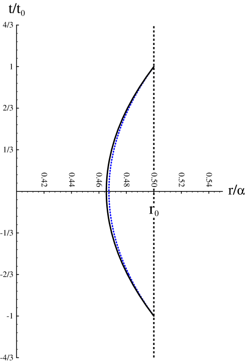
FIG. 1.: An exaggerated plot of the exact geodesic path (dotted line) and the parabolic approximation (solid line). $\alpha$ is the coordinate distance from $r=0$ to the horizon in the static de Sitter spacetime.

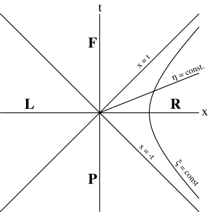
FIG. 2.: A plot of the Rindler coordinatization of two-dimensional Minkowski spacetime. The time coordinate $\eta=$ constant are straight lines passing through the origin, while the space coordinate $\xi=$ constant are hyperbolae. The Minkowski spacetime is covered by four separate coordinate patches, labeled by L, R, F and P. The two null rays ($x=t$ and $x=-t$) act as horizons.

REFERENCES

- [1] M. J. Pfenning and L. H. Ford, Phys. Rev. D 55, 4813 (1997), gr-qc/9608005.
- [2] L. H. Ford, Phys. Rev. D 43, 3972 (1991).
- [3] L. H. Ford and T. A. Roman, Phys. Rev. D 46, 1328 (1992).
- [4] L. H. Ford and T. A. Roman, Phys. Rev. D 51, 4277 (1995), gr-qc/9410043.
- [5] L. H. Ford and T. A. Roman, Phys. Rev. D 55, 2082 (1997), gr-qc/9607003.
- [6] L. H. Ford and T. A. Roman, Phys. Rev. D 53, 5496 (1996), gr-qc/9510071.
- [7] M. Alcubierre, Class. Quantum Grav. 11, L73 (1994).
- [8] M. J. Pfenning and L. H. Ford, Class. Quantum Grav. 14, 1743 (1997), gr-qc/9702026.
- [9] S. V. Krasnikov, Hyper-fast interstellar travel in general relativity, gr-qc/9511068 (unpublished).
- [10] A. Everett and T. A. Roman, Phys. Rev. D 56, 2100 (1997), gr-qc/9702049.
- [11] M. Visser, Phys. Rev. D 54, 5103 (1996), gr-qc/9604007.
- [12] M. Visser, Phys. Rev. D 54, 5116 (1996), gr-qc/9604008.
- [13] M. Visser, Phys. Rev. D 54, 5123 (1996), gr-qc/9604009.
- [14] M. Visser, Phys. Rev. D 56, 936 (1997), gr-qc/9703001.
- [15] M. R. Brown and A. C. Ottewill, Phys. Rev. D 34, 1776 (1986).
- [16] D.-Y. Song, Phys. Rev. D 55, 7586 (1997), gr-qc/9704001.
- [17] L. H. Ford, M. J. Pfenning, and T. A. Roman, Quantum inequalities and singular energy densities, in preparation.
- [18] L. H. Ford and N. F. Svaiter, in preparation.
- [19] S. A. Fulling, Aspects of Field Theory in Curved Space-Time (Cambridge University Press, Cambridge, 1989), p. 105.
- [20] N. D. Birrell and P. C. W. Davies, Quantum Fields in Curved Space, Cambridge Monographs on Mathematical Physics (Cambridge University Press, Cambridge, 1982).
- [21] D. Lohiya and N. Panchapakesan, J. Phys. A 11, 1963 (1978).
- [22] A. S. Lapedes, J. Math. Phys. 19, 2289 (1978).
- [23] A. Higuchi, Class. Quantum Grav. 4, 721 (1987).
- [24] H.-T. Sato and H. Suzuki, Mod. Phys. Let. A 9, 3673 (1994).
- [25] A. Kaiser and A. Chodos, Phys. Rev. D 52, 787 (1996).
- [26] I. S. Gradshteyn and I. M. Ryzhik, Table of Integrals, Series, and Products, fifth ed. (Academic Press, San Diego, 1994).
- [27] J. D. Jackson, Classical Electrodynamics, 2nd ed. (John Wiley & Sons, New York, 1975), see section 3.6.
- [28] Éanna É. Flanagan, Quantum inequalities in two-dimensional Minkowski Spacetime, gr-qc/9706006 in press.
- [29] B. S. DeWitt, Phys. Rep. 19c, 295 (1975).
- [30] P. Candelas, Phys. Rev. D 21, 2185 (1980).
- [31] B. P. Jenson, J. G. Mc Laughlin, and A. C. Ottewill, Phys. Rev. D 45, 3002 (1992).