Impulsive waves in de Sitter and anti-de Sitter space-times generated by null particles with an arbitrary multipole structure

Abstract

We describe a class of impulsive gravitational waves which propagate either in a de Sitter or an anti-de Sitter background. They are conformal to impulsive waves of Kundt’s class. In a background with positive cosmological constant they are spherical (but non-expanding) waves generated by pairs of particles with arbitrary multipole structure propagating in opposite directions. When the cosmological constant is negative, they are hyperboloidal waves generated by a null particle of the same type. In this case, they are included in the impulsive limit of a class of solutions described by Siklos that are conformal to pp-waves.

PACS class 04.20.Jb, 04.30.Nk

Running title: Impulsive waves in (anti-)de Sitter space-time

1 Introduction

We consider a particular class of exact solutions of Einstein’s equations which describe impulsive gravitational or matter waves in a de Sitter or an anti-de Sitter background. One class of such solutions has recently been derived by Hotta and Tanaka [1] and analysed in more detail elsewhere [2]. This was initially obtained by boosting the source of the Schwarzschild–(anti-)de Sitter solution in the limit in which its speed approaches that of light while its mass is reduced to zero in an appropriate way. In a de Sitter background, the resulting solution describes a spherical impulsive gravitational wave generated by two null particles propagating in opposite directions. In an anti-de Sitter background which contains closed timelike lines, the impulsive wave is located on a hyperboloidal surface at any time and the source is a single null particle with propagates from one side of the universe to the other and then returns in an endless cycle.

In this paper we investigate a more general class of such solutions. The global structure of the space-times and the shape of the impulsive wave surfaces are exactly as summarised above and described in detail in [2]. Here we consider a wider range of possible sources. We present an interesting class of impulsive gravitational waves that are also generated by null particles, but these particles in general can have an arbitrary multipole structure. The space-times are conformal to the impulsive limit of a family of type N solutions of Kundt’s class [3]. When the cosmological constant is negative, the solutions given here can be related to the impulsive limit of a class of solutions previously given by Siklos [4].

It may be noted that a family of impulsive spherical gravitational waves have also been obtained by Hogan [5]. These are particular (impulsive) cases of the Robinson–Trautman family of solutions with a cosmological constant. They will be discussed further elsewhere and are not related to the solutions given here.

As is well known, the de Sitter and anti-de Sitter space-times can naturally be represented as four-dimensional hyperboloids embedded in five-dimensional Minkowski spaces. Impulsive waves can easily be introduced into these space-times using this formalism. This is done is section 2 in which the form of the solution is constructed explicitly and the nature of its source is described. Appropriate coordinate systems for the separate cases of de Sitter and anti-de Sitter backgrounds are described respectively in sections 3 and 4 together with a discussion of the geometrical properties of the waves. Their relation to previously known solutions is indicated in section 5.

2 An impulsive gravitational wave in a space-time with a cosmological constant

We wish to consider impulsive waves in a de Sitter or an anti-de Sitter background. In these cases, the background can be represented as a four-dimensional hyperboloid

$${Z_{0}}^{2}-{Z_{1}}^{2}-{Z_{2}}^{2}-{Z_{3}}^{2}-\epsilon{Z_{4}}^{2}=-\epsilon a^{2}$$ (1)

embedded in a five-dimensional Minkowski space-time

$${\rm d}s^{2}={\rm d}{Z_{0}}^{2}-{\rm d}{Z_{1}}^{2}-{\rm d}{Z_{2}}^{2}-{\rm d}{Z_{3}}^{2}-\epsilon{\rm d}{Z_{4}}^{2}$$

where $a^{2}=3/\epsilon\Lambda$ for a cosmological constant $\Lambda$, $\epsilon=1$ for a de Sitter background ($\Lambda>0$), and $\epsilon=-1$ for an anti-de Sitter background ($\Lambda<0$) in which there are two timelike coordinates $Z_{0}$ and $Z_{4}$. Let us now consider a plane impulsive wave in this 5-dimensional Minkowski background. Without loss of generality, we may consider this to be located on the null hypersurface given by

$$Z_{0}+Z_{1}=0,\qquad{Z_{2}}^{2}+{Z_{3}}^{2}+\epsilon{Z_{4}}^{2}=\epsilon a^{2}.$$ (2)

so that the surface has constant curvature. For $\epsilon=1$, the impulsive wave is a 2-sphere in the 5-dimensional Minkowski space at any time $Z_{0}$. Alternatively, for $\epsilon=-1$, it is a 2-dimensional hyperboloid. The geometry of these surfaces has been described in detail elsewhere [2] using various natural coordinate systems.

In this five-dimensional notation, we consider the class of complete space-times that contain an impulsive wave on this background and that can be represented in the form

$${\rm d}s^{2} = {\rm d}{Z_{0}}^{2}-{\rm d}{Z_{1}}^{2}-{\rm d}{Z_{2}}^{2}-{\rm d}{Z_{3}}^{2}-\epsilon{\rm d}{Z_{4}}^{2}$$ (3)

$$\qquad-H(Z_{2},Z_{3},Z_{4})\delta(Z_{0}+Z_{1})({\rm d}Z_{0}+{\rm d}Z_{1})^{2}$$

where $H(Z_{2},Z_{3},Z_{4})$ is determined on the wave surface (2). Thus, $H$ must be a function of two parameters which span the surface. An appropriate parameterisation of this surface is given by

$$Z_{2}=a\sqrt{\epsilon(1-z^{2})}\cos\phi,\qquad Z_{3}=a\sqrt{\epsilon(1-z^{2})}\sin\phi,\qquad Z_{4}=az$$ (4)

where $|z|\leq 1$ when $\epsilon=1$ and $|z|\geq 1$ when $\epsilon=-1$. In terms of these parameters, it can be shown that the function $H(z,\phi)$ must satisfy the linear partial differential equation

$$(1-z^{2})H_{zz}-2zH_{z}+{1\over 1-z^{2}}H_{\phi\phi}+2H=-\epsilon 8\pi J(z,\phi)$$ (5)

where $J(z,\phi)$ represents the source of the wave. It is a remarkable fact that this equation arises in such a similar form for both de Sitter and anti-de Sitter backgrounds. This equation will be derived separately for both cases in the following sections.

It may immediately be observed that a solution of (5) of the form $H=$ const. represents a uniform distribution of null matter over the impulsive surface. This may always be added to any other non-trivial solution. However, from now on we will only consider solutions which are vacuum everywhere except for some possible isolated sources.

Let us now consider solutions that can be separated in the form

$$H_{m}(z,\phi)=H(z)e^{im\phi}$$

where $m$ is a real constant. Since $\phi$ is a periodic coordinate it follows that, for continuous solutions (except possibly at the poles $z=\pm 1$), $m$ must be a non-negative integer. For a vacuum solution with this condition, (5) reduces to an associated Legendre equation

$$(1-z^{2})H_{zz}-2zH_{z}-{m^{2}\over 1-z^{2}}H+2H=0.$$ (6)

This has the general solution

$$H(z)=a_{m}P^{m}_{1}(z)+b_{m}Q^{m}_{1}(z)$$

where $P^{m}_{1}(z)$ and $Q^{m}_{1}(z)$ are associated Legendre functions of the first and second kind of degree 1, and $a_{m}$ and $b_{m}$ are arbitrary constants.

The only possible nonsingular solutions involve the associated Legendre functions of the first kind. These are nonzero here only for $m=0,1$, and the solutions are given by

$$H(z,\phi)=a_{0}P^{0}_{1}(z)=a_{0}z,\qquad{\rm and}\qquad H(z,\phi)=a_{1}P^{1}_{1}(z)e^{i\phi}=-\epsilon a_{1}\sqrt{|1-z^{2}|}e^{i\phi}$$

or any linear combination of them. It may then be observed that the second of the above expressions can be obtained from the first by a simple “rotation” of the coordinates on the wave surface (2), so that they are essentially the same solution. We can thus restrict attention to the space-time (3) with $H={a_{0}\over a}Z_{4}$. It can then be shown that this case is conformally flat. The impulsive component in (3) can be removed by the discontinuous linear transformation

$$Z_{4} \to Z_{4}-\epsilon{a_{0}\over 2a}U\Theta(U)$$

$$V \to V+\epsilon{a_{0}^{2}\over 4a^{2}}U\Theta(U)-{a_{0}\over a}Z_{4}\Theta(U)$$

where $U\equiv Z_{0}+Z_{1}$, $V\equiv Z_{0}-Z_{1}$ and $\Theta$ is the Heaviside step function. (This does not introduce impulsive components into the Weyl tensor.) Thus, these nonsingular solutions represent only the de Sitter or anti-de Sitter backgrounds in different coordinates. In these backgrounds, there is no equivalent to the plane impulsive gravitational wave (for $\Lambda=0$) for which the Weyl tensor has constant components over the wave surface.

It now follows that the only nontrivial solution of (6) involves the Legendre functions of the second kind. These necessarily have singularities at $z=\pm 1$ which may correspond to poles at which the sources of the impulsive wave may be located. Summing over all possible modes, a general real solution is obtained in the form

$$H(z,\phi)=\sum_{m=0}^{\infty}b_{m}H_{m}(z,\phi)=\sum_{m=0}^{\infty}b_{m}Q^{m}_{1}(z)\cos[m(\phi-\phi_{m})]$$ (7)

where $b_{m}$ and $\phi_{m}$ are real constants representing the arbitrary amplitude and phase of each component. It may be recalled that the associated Legendre functions of the second kind are generated by the relation

$$Q^{m}_{1}(z)=(-\epsilon)^{m}|1-z^{2}|^{m/2}{{\rm d}^{m}\over{\rm d}z^{m}}Q_{1}(z)$$

where $Q_{1}(z)=Q^{0}_{1}(z)$. The first few of these functions are given by

$$Q_{1}^{0}(z) = {z\over 2}\log\left|{1+z\over 1-z}\right|-1,$$

$$Q_{1}^{1}(z) = -\epsilon{1\over 2}\sqrt{|1-z^{2}|}\log\left|{1+z\over 1-z}\right|-{z\over\sqrt{|1-z^{2}|}},$$ (8)

$$Q_{1}^{2}(z) = \epsilon{2\over 1-z^{2}},\qquad\qquad Q_{1}^{3}(z)=-{8z\over|1-z^{2}|^{3/2}}$$

which have been expressed in forms that are applicable for real $z$ for both $-1\leq z\leq 1$ and $|z|>1$.

The first of these terms ($m=0$) gives the simplest (axially symmetric) solution

$$b_{0}H_{0}={b_{0}\over 2a}\left[Z_{4}\log\left|{a+Z_{4}\over a-Z_{4}}\right|-2a\right].$$

In fact this is exactly the solution found by Hotta and Tanaka [1] (with $b_{0}=8p$) which was obtained by boosting the source of the Schwarzschild–(anti-)de Sitter space-time to the ultrarelativistic limit. In this case, the singularities correspond to sources represented by two delta functions

$$b_{0}J_{0}(z,\phi)=\epsilon{b_{0}\over 8\pi}\big{[}\delta(z-1)+\delta(z+1)\big{]}.$$

Let us now consider the further terms for arbitrary $m$. From the definition of $H_{m}(z,\phi)$ given in (7) and the identity (34) from the appendix, it can be shown that

$$(1-z^{2})H_{m,zz}-2zH_{m,z}+{1\over 1-z^{2}}H_{m,\phi\phi}+2H_{m}$$

$$\qquad=-(-1)^{m}(1-z^{2})^{m/2}\left[\delta^{(m)}(z-1)+\delta^{(m)}(-z-1)\right]\cos[m(\phi-\phi_{m})]$$

where $\delta^{(m)}$ is the $m^{\rm th}$ derivative of the delta function. Comparing this with (5), it can be seen that each of the components $H_{m}$ corresponds to sources at $z=\pm 1$ given by

$$J_{m}(z,\phi)=\epsilon{(-1)^{m}\over 8\pi}(1-z^{2})^{m/2}\left[\delta^{(m)}(z-1)+\delta^{(m)}(-z-1)\right]\cos[m(\phi-\phi_{m})].$$ (9)

These components describe point sources with an $m$-pole structure. They have the appropriate dependence on $z$ as the $m^{\rm th}$ derivative of the delta function, together with the appropriate periodic dependence on $\phi$. The multipole character of first three of these modes is clearly illustrated in Fig. 1. (It may be noted that similar multipole sources can generate impulsive pp-waves in space-times with $\Lambda=0$ [6].)

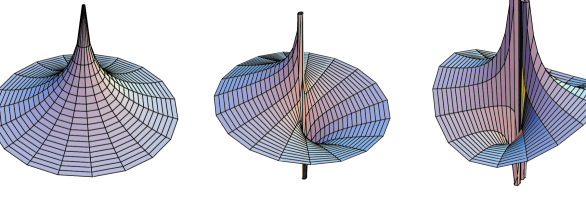
Figure 1: These pictures illustrate the monopole, dipole and quadrupole modes showing the dependence of the functions $H_{0}$, $H_{1}$ and $H_{2}$ near the singular point representing one of the sources of the impulsive waves.

Finally we observe that the solution (7) represents a general solution containing point sources which are arbitrary combinations of $m$-poles

$$J(z,\phi)=\sum_{m=0}^{\infty}b_{m}J_{m}(z,\phi).$$

The constants $b_{m}$ represent the strength of each $m$-pole and $\phi_{m}$ its orientation.

3 Impulsive waves in a de Sitter background

When the cosmological constant is positive, it is most convenient to work with the global coordinate system given by

$$Z_{0} = -a\cot\eta$$

$$Z_{1} = a\,{\rm cosec}\,\eta\cos\chi$$

$$Z_{2} = a\,{\rm cosec}\,\eta\sin\chi\sin\theta\cos\phi$$ (10)

$$Z_{3} = a\,{\rm cosec}\,\eta\sin\chi\sin\theta\sin\phi$$

$$Z_{4} = a\,{\rm cosec}\,\eta\sin\chi\cos\theta$$

in which $\eta,\chi,\theta\in[0,\pi]$, $\phi\in[0,2\pi]$. In these coordinates it can be seen that the impulsive wave is localised on the surface given by $\delta(Z_{0}+Z_{1})={1\over a}\delta(\chi-\eta)$. Thus, on the impulsive null hypersurface $\chi=\eta$ the coordinates (10) are identical to those of (4) with the identity $z=\cos\theta$.

In this case the line element (3) with the solution (7) takes the form

$${\rm d}s^{2}={a^{2}\over\sin^{2}\eta}\bigg{(}{\rm d}\eta^{2}-{\rm d}\chi^{2}-\sin^{2}\chi({\rm d}\theta^{2}+\sin^{2}\theta{\rm d}\phi^{2})\bigg{)}-aH(\theta,\phi)\,\delta(\eta-\chi)({\rm d}\eta-{\rm d}\chi)^{2}.$$ (11)

Now, in order to justify the equation (5), we may adapt the approach of Dray and ’t Hooft [7]. In deriving an exact solution for a spherical impulsive wave in a Schwarzschild space-time, they have given field equations for such a wave in a more general class of backgrounds. These also apply in a space-time with a positive cosmological constant. Using a line element of the form

$${\rm d}s^{2}=-2A(u,v){\rm d}u\big{[}{\rm d}v+H(\theta,\phi)\delta(u){\rm d}u\big{]}-g(u,v)({\rm d}\theta^{2}+\sin^{2}\theta{\rm d}\phi^{2})$$ (12)

and requiring that $A_{v}=0=A_{vv}$ and $g_{v}=0=g_{vv}$ on the null hypersurface $u=0$, the field equations given in [7] and [1] reduce to the single equation on the impulse

$$\left({A\over g}\Delta-{g_{uv}\over g}\right)\,H=8\pi J(\theta,\phi)$$ (13)

where $\Delta$ is the laplacian on the sphere and the source of the wave is given by $T_{uu}=J(\theta,\phi)\delta(u)$. Now, putting $u\equiv\chi-\eta$ and $v\equiv\cot[{1\over 2}(\chi+\eta)]$, the line element (11) can be transformed to the form (12) where $A$ and $g$ are given by

$$A(u,v)=-{a^{2}\over(1+v^{2})}{1\over\sin^{2}(\cot^{-1}v-u/2)},\qquad g(u,v)=a^{2}{\sin^{2}(\cot^{-1}v+u/2)\over\sin^{2}(\cot^{-1}v-u/2)}.$$

With these, (13) takes the explicit form

$$\left(\Delta+2\right)\,H(\theta,\phi)=-8\pi J(\theta,\phi).$$ (14)

Making the substitution $z\equiv\cos\theta$, the laplacian on a sphere becomes

$$\Delta=\partial_{z}\big{[}(1-z^{2})\partial_{z}\big{]}+(1-z^{2})^{-1}\partial_{\phi}\partial_{\phi}$$

with which (14) takes the form (5) which is thus established for this case.

We now consider the explicit solutions (7) given by

$$H(\theta,\phi)=\sum_{m=0}^{\infty}b_{m}H_{m}(\theta,\phi)=\sum_{m=0}^{\infty}b_{m}Q^{m}_{1}(\cos\theta)\cos[m(\phi-\phi_{m})].$$ (15)

The simplest case in which $b_{m}=0$ for $m>0$, is exactly the solution

$$H_{0}={1\over 2}\cos\theta\log\left({1+\cos\theta\over 1-\cos\theta}\right)-1$$

obtained by Hotta and Tanaka [1] as described elsewhere [2]. It represents a spherical impulsive wave in a de Sitter background generated by two null particles moving in opposite directions. The particles are situated at the poles $\theta=0$ and $\theta=\pi$. Using these global coordinates, it can be seen that the impulsive wave is located on the cosmological horizon of a de Sitter space-time. (This is analogous to the solution given in [7] in which the impulsive wave is located on the horizon of a Schwarzschild space-time.) Moreover, since $\chi=\eta$ on the wave, it can be seen from (11) that at any time the area of the spherical wavefront spanned by $\theta$ and $\phi$ is a constant equal to $4\pi a^{2}$. In fact it describes a spherical impulsive wave propagating from the North pole to the South pole in a closed form of the de Sitter universe which contracts to a minimum size and then re-expands as described in [1] and [2].

The general solution (15) of the space-time (11) can be seen to represent a similar wave generated by two null particles with arbitrary multipole structure. The first few higher multipole terms are given simply by

$$H_{1} = -\left[{1\over 2}\sin\theta\,\log\left({1+\cos\theta\over 1-\cos\theta}\right)+\cot\theta\right]\cos(\phi-\phi_{1})$$

$$H_{2} = {2\over\sin^{2}\theta}\cos[2(\phi-\phi_{2})]$$

$$H_{3} = -8{\cos\theta\over\sin^{3}\theta}\cos[3(\phi-\phi_{3})].$$

It has been argued above that the area of the spherical wavefront spanned by $\theta$ and $\phi$ is a constant. Therefore this particular wave is non-expanding (with the background either expanding or contracting through it). In view of this property, we would expect that this solution can be related to a particular (impulsive) case of the generalised class of Kundt waves with non-vanishing cosmological constant $K(\Lambda)$ presented by García Díaz and Plebański [8]. This has also been described by Ozsváth, Robinson and Rózga [9] as their class $R(\Lambda,0,1)$. Adapting the coordinate system of [9], the line element for this class of solutions can be given in the form

$${\rm d}s^{2}=2\left({\xi+\bar{\xi}\over 1+c\xi\bar{\xi}}\right)^{2}{\rm d}\tilde{u}{\rm d}\tilde{v}-{2{\rm d}\xi{\rm d}\bar{\xi}\over(1+c\xi\bar{\xi})^{2}}-\left[2\left({\xi+\bar{\xi}\over 1+c\xi\bar{\xi}}\right)^{2}\tilde{v}^{2}-{\xi+\bar{\xi}\over 1+c\xi\bar{\xi}}G\right]{\rm d}\tilde{u}^{2}$$ (16)

where $c=\Lambda/6$ and $G(\xi,\bar{\xi},\tilde{u})$ is required to satisfy the equation

$${1\over c}(1+c\xi\bar{\xi})^{2}G_{\xi\bar{\xi}}+2G={8\pi\over c}{1+c\xi\bar{\xi}\over\xi+\bar{\xi}}T_{\tilde{u}\tilde{u}}.$$ (17)

It may be observed that this class is conformal to Kundt’s class of type N vacuum solutions with vanishing cosmological constant [3]. In fact it can be shown [10] that this is the only class of vacuum solutions that are conformal to Kundt’s class of type N with $\Lambda$ zero.

Since this is just the de Sitter space-time when $G=0$ and $\Lambda>0$, we can concentrate here on the case of an impulsive wave in which $G(\xi,\bar{\xi},\tilde{u})=-H(\xi,\bar{\xi})\delta(\tilde{u})$. Now performing the transformation

$$\xi=\sqrt{2}a\tan{{\theta\over 2}}\>e^{i\phi},\qquad\qquad\tilde{v}={a\over\sqrt{2}}{1\over t},\qquad\qquad\tilde{u}={1\over\sqrt{2}a}(\rho-t),$$

where $a=1/\sqrt{2c}$ in this case, the line element (16) becomes

$${\rm d}s^{2}=a^{2}t^{-2}\sin^{2}\theta\cos^{2}\phi\>({\rm d}t^{2}-{\rm d}\rho^{2})-a^{2}({\rm d}\theta^{2}+\sin^{2}\theta{\rm d}\phi^{2})$$

$$\qquad\qquad\qquad-\sin\theta\cos\phi\,H(\theta,\phi)\delta(\rho-t)({\rm d}\rho-{\rm d}t)^{2}.$$ (18)

This can be seen to be exactly the solution (3) in which the de Sitter background in the five-dimensional form (1) is parameterised by

$$Z_{0} = -a\cos\theta+{a^{2}\over t}\sin\theta\cos\phi+{\rho^{2}-t^{2}\over 2t}\sin\theta\cos\phi$$

$$Z_{1} = \quad a\cos\theta-{a^{2}\over t}\sin\theta\cos\phi$$

$$Z_{2} = {\rho\over t}\>a\sin\theta\cos\phi$$ (19)

$$Z_{3} = \quad a\sin\theta\sin\phi$$

$$Z_{4} = \quad a\cos\theta\hskip 72.0pt-{\rho^{2}-t^{2}\over 2t}\sin\theta\cos\phi$$

where, for consistency with (4) we only need to consider the impulsive wave located on $\rho=t$. In addition, the field equation (17) is identical to (5).

Finally, we may note that the left hand side of equation (14) or (17) is just the laplacian over the sphere plus two operating on a function. It follows that the solutions described above can be rotated arbitrarily over the sphere. Since the equation is linear, solutions can therefore be constructed which contain an arbitrary number of pairs of arbitrary multipole particles distributed arbitrarily over the impulsive spherical wave. However, the impulsive wave is unique — it is a sphere of constant surface area equal to $4\pi a^{2}$.

4 Impulsive waves in an anti-de Sitter background

When the cosmological constant is negative, it is most convenient to introduce the global coordinate system given by

$$Z_{0} = a(\cosh R+\sinh R\cos\phi)\eta$$

$$Z_{1} = a(\cosh R+\sinh R\cos\phi)\chi$$

$$Z_{2} = a\sinh R\cos\phi-{\textstyle{1\over 2}}a(\cosh R+\sinh R\cos\phi)(\chi^{2}-\eta^{2})$$ (20)

$$Z_{3} = a\sinh R\sin\phi$$

$$Z_{4} = a\cosh R\hskip 24.0pt+{\textstyle{1\over 2}}a(\cosh R+\sinh R\cos\phi)(\chi^{2}-\eta^{2})$$

in which $\chi,\eta\in(-\infty,\infty)$, $R\in(0,\infty)$ and $\phi\in[0,2\pi)$. Although this coordinate system is unconventional, it is particularly convenient for our purposes here. In these coordinates it can be seen that the impulsive wave is localised on the surface given by $\delta(Z_{0}+Z_{1})={1\over a}(\cosh R+\sinh R\cos\phi)^{-1}\delta(\chi+\eta)$. Thus, on the impulsive null hypersurface $\chi+\eta=0$, the coordinates (20) are identical to those of (4) with the identity $z=\cosh R$.

In this case the general line element (3) for an impulsive wave in an anti-de Sitter background takes the form

$${\rm d}s^{2} = a^{2}(\cosh R+\sinh R\cos\phi)^{2}\big{(}{\rm d}\eta^{2}-{\rm d}\chi^{2}\big{)}-a^{2}\big{(}{\rm d}R^{2}+\sinh^{2}R{\rm d}\phi^{2}\big{)}$$ (21)

$$\qquad-a(\cosh R+\sinh R\cos\phi)\,H(R,\phi)\,\delta(\eta+\chi)({\rm d}\eta+{\rm d}\chi)^{2}.$$

It may immediately be observed that these coordinates are naturally adapted such that the impulsive wave is given by $\chi+\eta=0$, and that the wave surface of a constant negative curvature which is spanned by the parameters $R$ and $\phi$ do not vary with time. The geometrical properties of these waves have been described elsewhere [2] using different coordinate systems. Basically, the impulsive wave is hyperboloidal and is generated by a single null particle moving in an anti-de Sitter background which contains closed timelike geodesics. The particle propagates from one side of the universe to the other and then returns in an endless cycle. The wave propagating in one direction is obtained by the parameterisation $z=\cosh R$ as above, while propagation in the opposite direction can be parameterised by changing the signs of $Z_{2}$, $Z_{3}$ and $Z_{4}$ in (20) which is equivalent to putting $z=-\cosh(-R)$.

It is also convenient to reparameterise the wave surfaces by introducing an alternative global coordinate system in which

$$x={a\over\cosh R+\sinh R\cos\phi},\qquad y={a\sinh R\sin\phi\over\cosh R+\sinh R\cos\phi}.$$ (22)

Then, also putting $\tilde{\eta}=a\eta$ and $\tilde{\chi}=a\chi$, (21) becomes

$${\rm d}s^{2}={a^{2}\over x^{2}}\left({\rm d}\tilde{\eta}^{2}-{\rm d}\tilde{\chi}^{2}-{\rm d}x^{2}-{\rm d}y^{2}-{x\over a}\,H(x,y)\,\delta(\tilde{\eta}+\tilde{\chi})({\rm d}\tilde{\eta}+{\rm d}\tilde{\chi})^{2}\right).$$ (23)

In these coordinates, the parameterisation of (1) with $\epsilon=-1$ is given by

$$Z_{0}={a\over x}\tilde{\eta},\qquad Z_{1}={a\over x}\tilde{\chi},\qquad Z_{2}={1\over 2x}\big{(}a^{2}+\tilde{\eta}^{2}-x^{2}-y^{2}-\tilde{\chi}^{2}\big{)},$$ (24)

$$Z_{3}={a\over x}y,\qquad Z_{4}={1\over 2x}\big{(}a^{2}-\tilde{\eta}^{2}+x^{2}+y^{2}+\tilde{\chi}^{2}\big{)}$$

It may immediately be observed that (23) is conformal to an impulsive pp-wave. In fact it is the impulsive member of a family of solutions described by Siklos [4] which include the only vacuum space-times that are conformal to pp-waves. In this work, Siklos found a specific family of exact type N solutions (including possible pure radiation) with a negative cosmological constant given by

$${\rm d}s^{2}={a^{2}\over x^{2}}\left({\rm d}\tilde{\eta}^{2}-{\rm d}\tilde{\chi}^{2}-{\rm d}x^{2}-{\rm d}y^{2}-S(x,y,\tilde{\eta}+\tilde{\chi})({\rm d}\tilde{\eta}+{\rm d}\tilde{\chi})^{2}\right)$$ (25)

provided $S$ satisfies the equation

$$S_{xx}+S_{yy}-{2\over x}S_{x}=-16\pi T_{\tilde{u}\tilde{u}}$$ (26)

where $\tilde{u}=\tilde{\eta}+\tilde{\chi}$. Since the left hand side does not depend on $\tilde{u}$ explicitly, an arbitrary wave profile may be assumed and the solutions considered here simply correspond to the impulsive case in which $T_{\tilde{u}\tilde{u}}=J(x,y)\delta(\tilde{\eta}+\tilde{\chi})$. Putting

$$S={x\over a}H(x,y)\delta(\tilde{\eta}+\tilde{\chi}),$$ (27)

equation (26) can be written as $-x^{2}(H_{xx}+H_{yy})+2H=16\pi axJ(x,y)$ which, using the coordinates $z=\cosh R$ and $\phi$ given by (22), may be confirmed to be exactly of the form (5). Equation (5) is thus justified also for the case of a negative cosmological constant.

Having established the equation (5) in this case, we now express the explicit solutions (7) in the form

$$H(R,\phi)=\sum_{m=0}^{\infty}b_{m}H_{m}(R,\phi)=\sum_{m=0}^{\infty}b_{m}Q^{m}_{1}(\cosh R)\cos[m(\phi-\phi_{m})].$$ (28)

This now clearly represents an impulsive gravitational wave on a null hyperboloidal surface generated by a single null particle of arbitrary multipole structure located at the point $R=0$ on the surface.

As in the previous section, we may finally note that the field equation is linear and includes the laplacian over a hyperboloidal surface of constant negative curvature. It therefore again follows that solutions can be constructed which contain an arbitrary number of arbitrary multipole particles distributed arbitrarily over the impulsive wave surface.

5 Further remarks

In his paper [4], Siklos has also shown that, for the vacuum case (except for some possible point sources), the general solutions of (26) for $S$ is of the form

$$S=x^{2}{\partial\over\partial x}\left({f+\bar{f}\over x}\right)$$ (29)

where $f=f(\zeta,\tilde{u})$ is an arbitrary function of $\zeta=x+iy$ and $\tilde{u}=\tilde{\eta}+\tilde{\chi}$ (holomorphic in $\zeta$). For space-times that are conformal to Kundt waves for both positive and negative cosmological constant, Ozsváth, Robinson and Rózga [9] have presented the equivalent explicit vacuum solution to their equation (17) which also involves an arbitrary function which is holomorphic in $\xi$ which is related to $\zeta$ by

$$\zeta={1-\sqrt{c}\,\xi\over 1+\sqrt{c}\,\xi}.$$

Using (29) and also (22) with $z=\cosh R$, a general vacuum solution of (5) can be written as

$${1\over a}\,H(\zeta,\bar{\zeta})=f_{\zeta}+\bar{f}_{\bar{\zeta}}-2{f+\bar{f}\over\zeta+\bar{\zeta}}$$

where $f=f(\zeta)$. In terms of the coordinates $z$ and $\phi$, $\zeta$ is given by

$$\zeta=a{1+i\sqrt{z^{2}-1}\sin\phi\over z+\sqrt{z^{2}-1}\cos\phi}.$$

The explicit solutions described in the current paper may easily be represented in this form. For these cases, The Siklos function $S$ may be expressed as $S=b_{m}\sum_{m}S_{m}(x,y)\delta(\tilde{u})$, where $S_{m}$ corresponds to the distinct $m$-pole modes $H_{m}$. For completeness, we may now identify the expressions corresponding to the first few modes described above. For $m=0$, the monopole solution for $H_{0}$ is equivalent to

$$S_{0}(x,y)={1\over 4a^{2}}\left[(a^{2}+x^{2}+y^{2})\log{(x+a)^{2}+y^{2}\over(x-a)^{2}+y^{2}}-4ax\right]$$

which corresponds to

$$f_{0}(\zeta)={1\over 4a^{2}}(\zeta^{2}-a^{2})\log{\zeta+a\over\zeta-a}.$$

When $m=1$, the dipole solution for $H_{1}$ is equivalent to

$$S_{1}(x,y)={1\over 4a^{2}}\left[\log{(x+a)^{2}+y^{2}\over(x-a)^{2}+y^{2}}-{4ax(a^{2}+x^{2}+y^{2})\over[(x+a)^{2}+y^{2}][(x-a)^{2}+y^{2}]}\right]$$

$$\hskip 156.0pt\times\big{[}(a^{2}-x^{2}-y^{2})\cos\phi_{1}+2ay\sin\phi_{1}\big{]}$$

which corresponds to

$$f_{1}(\zeta)=-{1\over 2a^{2}}\left[(\zeta-a)^{2}e^{i\phi_{1}}+(\zeta+a)^{2}e^{-i\phi_{1}}\right]\log{\zeta+a\over\zeta-a}.$$

When $m=2$, the quadrupole solution for $H_{2}$ is equivalent to

$$S_{2}(x,y)=8ax^{3}{\left[(a^{2}-x^{2}-y^{2})^{2}-4a^{2}y^{2}\right]\cos 2\phi_{2}+4ay(a^{2}-x^{2}-y^{2})\sin 2\phi_{2}\over[(x+a)^{2}+y^{2}]^{2}[(x-a)^{2}+y^{2}]^{2}}$$

which corresponds to

$$f_{2}(\zeta)=-a\left[{1\over\zeta+a}e^{2i\phi_{2}}+{1\over\zeta-a}e^{-2i\phi_{2}}\right].$$

Appendix

It is well known that, at least in the range $z\in[-1,1]$, any function can be expressed as a sum of Legendre polynomials. In particular, using the identity $\int_{-1}^{1}P_{j}(z)Q_{1}(z)\,{\rm d}z={1+(-1)^{j}\over j(j+1)-2}$, it can be shown that

$$Q_{1}(z)=\sum_{j=0}^{\infty}{j+{1\over 2}\over j(j+1)-2}\left[P_{j}(z)+P_{j}(-z)\right].$$ (30)

It also follows immediately from the closure property of the set of Legendre polynomials that

$$\delta(z-1)=\sum_{j=0}^{\infty}(j+{\textstyle{1\over 2}})P_{j}(z).$$ (31)

The associated Legendre functions are generated by the relations

$$P^{m}_{j}(z)\equiv(-1)^{m}(1-z^{2})^{m/2}{{\rm d}^{m}\over{\rm d}z^{m}}P_{j}(z),\qquad Q^{m}_{j}(z)\equiv(-1)^{m}(1-z^{2})^{m/2}{{\rm d}^{m}\over{\rm d}z^{m}}Q_{j}(z).$$ (32)

By differentiating (30) $m$ times and multiplying by $(-1)^{m}(1-z^{2})^{m/2}$, it can be shown that

$$Q_{1}^{m}(z)=\sum_{j=0}^{\infty}{j+{1\over 2}\over j(j+1)-2}\left[P_{j}^{m}(z)+(-1)^{m}P_{j}^{m}(-z)\right].$$ (33)

Now, let us introduce the operator $L_{m}\equiv(1-z^{2}){{\rm d}^{2}\over{\rm d}z^{2}}-2{{\rm d}\over{\rm d}z}-{m^{2}\over 1-z^{2}}$. Then, applying the identity $\big{[}L_{m}+j(j+1)\big{]}P_{j}^{m}(z)=0$ to (33), it can immediately be seen that

$$\big{(}L_{m}+2\big{)}Q_{1}^{m}(z)=-\sum_{j=0}^{\infty}(j+{\textstyle{1\over 2}})\left[P_{j}^{m}(z)+(-1)^{m}P_{j}^{m}(-z)\right].$$

Using the definition of $P_{j}^{m}(z)$ in (32), this becomes

$$\big{(}L_{m}+2\big{)}Q_{1}^{m}(z)=-(-1)^{m}(1-z^{2})^{m/2}{{\rm d}^{m}\over{\rm d}z^{m}}\sum_{j=0}^{\infty}(j+{\textstyle{1\over 2}})\left[P_{j}(z)+P_{j}(-z)\right]$$

and, from (31), we finally obtain that

$$\big{(}L_{m}+2\big{)}Q_{1}^{m}(z)=-(-1)^{m}(1-z^{2})^{m/2}\left[\delta^{(m)}(z-1)+\delta^{(m)}(-z-1)\right]$$ (34)

where $\delta^{(m)}$ is the $m^{\rm th}$ derivative of the delta function.

References

• [1] Hotta M and Tanaka M 1993 Class. Quantum Grav. 10, 307.
• [2] Podolský J and Griffiths J B 1997 Phys. Rev. D 56 to appear in Oct.
• [3] Kramer D, Stephani H, MacCallum M A H and Herlt E 1980 Exact solutions of Einstein’s field equations, Cambridge University Press, chapter 27.
• [4] Siklos S T C 1985 Galaxies, axisymmetric systems and relativity, Ed. M A H MacCallum, Cambridge University Press, 247.
• [5] Hogan P A 1992 Phys. Lett. A 171, 21.
• [6] Griffiths J B and Podolský J 1997 Phys. Lett. A to appear.
• [7] Dray T and ’t Hooft G 1985 Nucl. Phys. B 253, 173.
• [8] García Díaz A and Plebański J F 1981 J. Math. Phys. 22 2655.
• [9] Ozsváth I, Robinson I and Rózga K 1985 J. Math. Phys. 26 1755.
• [10] Podolský J 1993 PhD thesis, Charles University, Prague.