Evolving wormhole geometries

Abstract

We present here analytical solutions of General Relativity that describe evolving wormholes with a non-constant redshift function. We show that the matter that threads these wormholes is not necessarily exotic. Finally, we investigate some issues concerning WEC violation and human traversability in these time-dependent geometries.

PACS number(s): 04.20.-q, 04.20.Jb

I Introduction

In the last two decades, there has been a revival on the study of classical wormhole solutions either in General Relativity (GR) or in alternative theories of gravitation. A cornerstone in this revival has been the paper of Morris and Thorne [1] in which, they derived the properties that a space-time must have in order to hold up such a geometry. Let us recall that the most salient feature of these space-times is that an embedding of one of their space-like sections in euclidean space displays two asymptotically flat regions joined by a throat. There are several reasons that support the interest in these solutions. One of them is the possibility of constructing time machines [2, 3, 4] which violate Hawking’s chronology protection conjecture [5]. Another reason is related to the nature of the matter that generates this solution: it must be “exotic”, i.e. its energy density takes negative values in some reference systems. This entails violations of the weak energy condition (WEC) which, although not based in any strong physical evidence [6], is deep enough in the body of relativists’ belief so as to abandon it without serious reasons. These violations are in fact encoded in the evolution of the expansion scalar, governed by Raychaudhuri’s equation [7]. As WEC is violated for any static spherically symmetric wormhole and has recently been shown to be the case also for any static wormhole in GR [8], the attemps to get around WEC violations have led two different branches of research. Firstly, there have been an increasing number of works in non-standard gravity theories. Brans-Dicke gravity supports static wormholes both in vacuum [9] and with matter content that do not violate the WEC by itself [10]. Also, there are analysis in several others alternative gravitational theories, such as $R+R^{2}$ [11], Einstein-Gauss-Bonnet [12] and Einstein-Cartan models [13]. In all cases, the violation of WEC is a necessary condition for static wormhole to exist, although these changes in the gravitational action allows one to have normal matter while relegating the exoticity to non-standard fields. This lead to explore the issue of WEC violation in non-static situations and see which is the case for dynamic, time-dependent wormholes. The first of this kind of analysis, due to Roman [14], was devoted to the case of inflating Lorentzian wormholes. These are wormholes of the Morris-Thorne type embedded in an inflating background, with all non-temporal components of the metric tensor multiplied by a factor of the form $e^{2\chi t}$, being $\chi$ related to the cosmological constant. The aim of Roman was to show that a microscopical wormhole could be enlarged by inflationary processes. However, this construction also violate the WEC. The other works, due to Kar and Kar and Sahdev [15, 16], pointed at testing whether, within classical GR, a class of non-static, non-WEC-violating wormholes could exists. They used a metric with a conformal time-dependent factor, whose spacelike sections are $R\times S^{2}$ with a wormhole metric, like the ones analyzed in [1]. In this work, we shall extend this last analysis by studying more general cases of evolving wormholes, given by a generic Morris-Thorne metric, in the presence of matter described by a given stress-energy tensor. To proceed further we shall make two ansätze. Firstly, we give a specification of the redshift function $\Phi$ of Morris-Thorne consistent, for any hypersurface of constant $t$, with asymptotic flatness and a metric free of horizons, as was the one made for the static case in [17]. Then we shall show how to choose a particular functional form for the trace of the stress-energy tensor matter in order to get different solutions for the conformal factor. At this point, we shall derive an analytical solution which we use later to analyze the WEC violation scenario and some human tranversability criteria.

II Geometrical and topological features

We adopt the following diagonal metric for the space-time:

$$ds^{2}=\Omega(t)\,\{-e^{2\Phi(r)}dt^{2}+e^{2\Lambda(r)}dr^{2}+r^{2}d\Omega_{2}^{2}\}$$ (1)

with $\Omega(t)$ a conformal factor, finite and positive defined throughout the domain of $t$, and $d\Omega_{2}^{2}$, the $S^{2}$ line element as usual. When $\Omega(t)$ is constant, this general metric stands for the ones firstly analyzed in the work of Morris and Thorne [1]. When $e^{2\Phi}=1$, it reduces to the particular case studied by Kar [15]. In the spirit of [17], we make the Ansatz $\Phi=-\alpha/r$, where $\alpha$ is a positive constant to be determined. This choice guarantees that the redshift function is finite everywhere, and consequently there is no event horizon. For the stress-energy tensor we take that of an imperfect fluid [18],

$$T_{\mu\nu}=(\rho+p)\,\xi_{\mu}\xi_{\nu}+p\,g_{\mu\nu}+\Delta p\left[\zeta_{\mu}\zeta_{\nu}-\frac{1}{3}\,(g_{\mu\nu}+\xi_{\mu}\xi_{\nu})\right]+2\,q\,\zeta_{(\mu}\xi_{\nu)}$$ (2)

where $\rho$ stands for the energy density, $p$ for the isotropic fluid pressure, and $q$ for the energy flux. The anisotropy pressure $\Delta p$ is the difference between the local radial ($p_{r}$) and lateral ($p_{\perp}$) stresses. With the foregoing assumptions, the nonvanishing Einstein’s equations are

$$\frac{3\,\dot{\Omega}^{2}\,e^{2\alpha/r}}{4\,\Omega^{3}}+\frac{2\,\Lambda^{\prime}\,e^{-2\Lambda}}{r\,\Omega}+\frac{1}{r^{2}\,\Omega}-\frac{e^{-2\Lambda}}{r^{2}\,\Omega}=8\pi\rho$$ (3)

$$\frac{3\,\dot{\Omega}^{2}\,e^{2\alpha/r}}{4\,\Omega^{3}}+\frac{2\,\alpha\,e^{-2\Lambda}}{r^{3}\,\Omega}-\frac{\ddot{\Omega}\,e^{2\alpha/r}}{\Omega^{2}}-\frac{1}{\Omega\,r^{2}}+\frac{e^{-2\Lambda}}{\Omega\,r^{2}}=8\pi p_{r}$$ (4)

$$\frac{3\,\dot{\Omega}^{2}\,e^{2\alpha/r}}{4\,\Omega^{3}}-\frac{\ddot{\Omega}\,e^{2\alpha/r}}{\Omega^{2}}-\frac{e^{-2\Lambda}\,\alpha}{r^{3}\,\Omega}-\frac{\Lambda^{\prime}\,e^{-2\Lambda}}{r\,\Omega}+\frac{\alpha^{2}\,e^{-2\Lambda}}{r^{4}\,\Omega}-\frac{\alpha\,\Lambda^{\prime}\,e^{-2\Lambda}}{\Omega\,r^{2}}=8\pi p_{\perp}$$ (5)

$$\frac{\dot{\Omega}\,\alpha}{r^{2}\,\Omega^{2}}=8\pi q\,\,e^{\Lambda}\,e^{\alpha/r}$$ (6)

In the expressions given above, dashes denote derivatives with respect to $r$ while dots, derivatives with respect to $t$. It seems convenient to assume that the trace of the stress energy tensor will be a separated function of $t$ and $r$,

$$T_{\mu}^{\mu}=\left[-3\frac{\ddot{\Omega}}{\Omega}+\frac{3}{2}\left(\frac{\dot{\Omega}}{\Omega}\right)^{2}\right]\frac{e^{2\alpha/r}}{\Omega}+\frac{1}{\Omega}\left\{-2\,e^{-2\Lambda}\left[\Lambda^{\prime}\left(\frac{2}{r}+\frac{\alpha}{r^{2}}\right)\right.\right. + \left.\left.\frac{e^{2\Lambda}}{r^{2}}-\frac{1}{r^{2}}-\frac{\alpha^{2}}{r^{4}}\right]\right\}$$ (7)

$$:= \Upsilon(t)\frac{e^{2\alpha/r}}{\Omega(t)}$$ (8)

After separating variables, equation (8) can be rewritten as,

$$-3\frac{\ddot{\Omega}}{\Omega}+\frac{3}{2}\left(\frac{\dot{\Omega}}{\Omega}\right)^{2}-\Upsilon={\cal C}$$ (9)

$$2\,e^{-2\alpha/r}\,e^{-2\Lambda}\left[\Lambda^{\prime}\left(\frac{2}{r}+\frac{\alpha}{r^{2}}\right)+\frac{e^{2\Lambda}}{r^{2}}-\frac{1}{r^{2}}-\frac{\alpha^{2}}{r^{4}}\right]={\cal C}$$ (10)

where ${\cal C}$ is an arbitrary constant which for simplicity, we shall take equal to 0. Performing the change of variables $\Lambda={\rm ln}z$, equation (10) transforms into a Bernoulli equation,

$$\frac{-z^{\prime}}{z}\left(\frac{2}{r}+\frac{\alpha}{r^{2}}\right)-\frac{z^{2}}{r^{2}}+\left(\frac{1}{r^{2}}+\frac{\alpha^{2}}{r^{4}}\right)=0.$$ (11)

The additional change $y=z^{-2}=\exp{[-2\Lambda]}$, allows for the general solution to be written as

$$y=e^{-2\Lambda}=\frac{\phi^{2}+9\phi^{3}+32\phi^{5}+(\,57/2+e^{2/\phi}\,{\cal K}\,)\phi^{4}}{(2\,\phi+1)^{5}}.$$ (12)

with $\phi=r/\alpha$, and ${\cal K}$ an integration constant to be determined. Note that, far from the wormhole throat,

$$\lim_{r\rightarrow\infty}e^{-2\Lambda}=1,$$ (13)

or equivalently,

$$\lim_{r\rightarrow\infty}\frac{dz}{dr}=0,$$ (14)

where $z(r)$ is the embedding function [1]. Moreover, for any hypersurface of constant $t$ the mouths of the wormhole need to connect two asymptotically flat spacetimes, thus the geometry at the wormhole’s throat is severely constrained. Indeed, the definition of the throat (minimum wormhole radius), entails for a vertical slope of the embedding surface,

$$\lim_{r\rightarrow r\th^{+}}\frac{dz}{dr}=\lim_{r\rightarrow r\th^{+}}\pm\sqrt{e^{2\Lambda}-1}=\infty;$$ (15)

besides, the solution must satisfy the flaring out condition [1], which stated mathematically reads,

$$-\frac{\Lambda^{\prime}e^{-2\Lambda}}{(1-e^{-2\Lambda})^{2}}>0.$$ (16)

Equations (15) and (16) will be satisfied if and only if

$$\lim_{\phi\rightarrow\phi\th^{{}^{+}}}e^{-2\Lambda}=0^{+},$$ (17)

thus, in order to fix the constant ${\cal K}$, we we must select a value for the dimensionless radius of the throat ($\phi\th>0$) such that Eq. (17) be satisfied. Nevertheless, the absolute size of the throat also depends on $\alpha$. As an example let us impose $\phi\th=2$ which, using (12), sets ${\cal K}=-97.25\,e^{-1}$ and $r\th=2\,\alpha$. The aforementioned properties of $\Lambda$, together with the definition of $\Phi$ and $\Omega$, entail that the metric tensor describes, for $\Omega(t)=$ constant, two asymptotically flat spacetimes joined by a throat. Thus, equation (12) represents an analytical solution for an evolving wormhole geometry, which, due to the choice we made for the trace, is independent of $\Omega(t)$. To obtain the complete behavior of the metric, we have to define $\Upsilon(t)$ in order to solve for $\Omega(t)$ in equation (9). We take instead Eq. (9) as the definition of $\Upsilon(t)$ in what follows.

III Avoiding WEC violations

Having at our disposal an explicit wormhole solution, given in the form of $y(\phi)$, we can now turn to the question of whether it entails WEC violations. Of course, we have to note that, in the general case, it will ultimately depend on the specific choice of $\Omega(t)$, but we use here the fact that, due to the form in which the solution for $y(\phi)$ was computed, it is independent of the explicit form of the conformal factor. Thus, we are able to study different functional forms of $\Omega(t)$ for the same $y(\phi)$. The WEC asserts that for any time-like vector $v^{\mu}$:

$$T_{\mu\nu}v^{\nu}v^{\mu}\geq 0.$$ (18)

The physical significance of this condition is that the observed energy density, as measured by any time-like observer, has to be positive. The connection of WEC violations with the existence of wormholes geometries has been widely studied before [2, 6, 8, 15]. In the case of evolving wormholes, Kar [15] has demonstrated that there exist wormhole solutions which do not violate the WEC for a specific choice of the redshift function. His analysis is indeed general, in the sense that even without having worked out any explicit wormhole solution, he could conclude that there exist some Lorentzian evolving wormhole geometries with the required matter not violating the WEC. We must recall however that Kar dealt with the particular case $\Phi=0$. We pursue here to refine his analysis, by means of the solution for the metric component $g_{11}$ given in the previous section. With the stress-energy tensor of equation (2), WEC entails

$$\rho\geq 0\;\;\;\;\;\;\;\rho\,+p_{r}+2\,q\geq 0\;\;\;\;\;\;\;\rho+p_{\perp}\geq 0.$$ (19)

Starting from the Einstein equations, the three previous inequalities can be written as follows:

$$f_{1}(t)+g_{1}(r)\geq 0\;\;\;\;\;\forall(t,r)$$ (20)

$$f_{2}(t)+g_{2}(r)+2\,q(r,t)\geq 0\;\;\;\;\;\forall(t,r)$$ (21)

$$f_{3}(t)+g_{3}(r)\geq 0\;\;\;\;\;\forall(t,r)$$ (22)

where the functions $f_{i}$ and $g_{i}$ are as in Table I. It is a trivial exercise to write all radial functions in terms of the $\phi$-variable by means of the definition $\phi=r/\alpha$. After this is done, it is seen that these functions display an explicit dependence on the $\alpha$ parameter and on $\phi\th$, through ${\cal K}$. The radius of the throat will be fixed when $\alpha$ and $\phi\th$ are simultaneously known. These radial functions are plotted in Figs. 1,2 and 3 for different values of $\alpha$ and for $\phi\th=2$. Note that, at or near the throat, some of them are negative. This just reflects the fact that no static wormholes can be built, within GR, without using exotic matter. Far enough from the throat, all functions tend to zero, being strong the dependence on $\alpha$ of the shape of the curves. Also from the figures, we may note that if we demand that the time-dependent functions $f_{1},f_{2}$ and $f_{3}$ be greater than the modulus of the minimum of each of the corresponding radial functions, all WEC inequalities will be fulfilled. In the case of the second inequality, the term coming from the energy flux must be taken into account to determine the non-exotic region. In Table II, we provide several examples of possible solutions for $\Omega(t)$. The procedure to obtain these particular functions as solutions for the metric is, as stated, to define a suitable functional form for the temporal part of the trace of the stress-energy tensor for matter, i.e. $\Upsilon(t)$. This values are also given together with the values of the temporal functions $f_{i}$ for each choice. This entries would allow comparison with WEC inequalities in order to search for constraints on the values of the constants involved in each choice of $\Omega(t)$, to be fulfilled in order to obtain non-exotic matter at the throat of the evolving wormhole. Finally, the domain of $t$ for which $\Omega$ is finite and without zeros is also given in Table II. The comments made by Kar [15] when he considered different $\Omega(t)$ functions in his scheme are totally applicable here. For instance, we also have exponentially expanding or contracting phases -for the first two solutions- and a wormhole -like universe (with a bang and a crunch) for $\Omega(t)=\sin^{2}(\omega t)$. In our scheme, the particular choice of $\Omega(t)$ will determine the energy flux, through the field equation (6). The sign of the energy flux (which depends on $\dot{\Omega}$) will decide in turn if the wormhole is attractive or repulsive, in the sense explained in [14]. For large enough and positive $q$, the second WEC inequality will be fulfilled easily. Morover, this would imply a quick process of expansion which in turn favors a possible trip by diminishing the tidal forces, as we shall show in the next section.

IV Traversability criteria

We shall deal now with the possibility that an explorer might enter into the kind of evolving wormhole studied here, pass through the tunnel, and exit into an external space again without being crushed during the journey. We are not going to discuss here the stability of the wormhole, being this beyond the scope of this paper. Instead, we content ourselves with an analysis of the tidal gravitational forces that an infalling radial observer must bear during the trip. The extension to a non-radial motion follows from the recipe given in [19] (Chap. 13). We recall the desired traversability criteria concerning the tidal forces that an observer should feel during the journey: they must not exceed the ones due to Earth gravity [20]. From now on, the algebra will be simplified by switching to an orthonormal reference frame in which $g_{\hat{\mu}\hat{\nu}}=\eta_{\hat{\mu}\hat{\nu}}$. In terms of this basis, the proper reference frame is given by,

$$e_{\hat{0}^{\prime}}=\gamma\,e_{\hat{t}}\mp\gamma\,\beta\,e_{\hat{r}}\hskip 28.45274pte_{\hat{1}^{\prime}}=\mp\,\gamma\,e_{\hat{r}}+\gamma\,\beta\,e_{\hat{t}}\hskip 28.45274pte_{\hat{2}^{\prime}}=e_{\hat{\theta}}\hskip 28.45274pte_{\hat{3}^{\prime}}=e_{\hat{\phi}}$$ (23)

where $\gamma$ and $\beta$ are the usual parameters of the Lorentz transformation formula. Thus, stated mathematically the traversability criteria read,

$$|R_{\hat{1}^{\prime}\hat{0}^{\prime}\hat{1}^{\prime}\hat{0}^{\prime}}|=\left|\frac{1}{\Omega}\left\{\frac{\alpha^{2}}{e^{2\Lambda}\,r^{4}}-\frac{2\,\alpha}{e^{2\Lambda}r^{3}}-\frac{\ddot{\Omega}\,e^{2\alpha/r}}{2\,\Omega}+\frac{\dot{\Omega}^{2}e^{2\alpha/r}}{2\,\Omega^{2}}-\frac{\alpha\,\Lambda^{\prime}}{e^{2\Lambda}r^{2}}\right\}\right|\leq\frac{g_{{}_{\oplus}}}{2m}\approx\frac{1}{(10^{10}{\rm cm})^{2}}$$ (24)

$$|R_{\hat{2}^{\prime}\hat{0}^{\prime}\hat{2}^{\prime}\hat{0}^{\prime}}|=|R_{\hat{3}^{\prime}\hat{0}^{\prime}\hat{3}^{\prime}\hat{0}^{\prime}}|=\gamma^{2}|R_{\hat{\theta}\hat{t}\hat{\theta}\hat{t}}|+\gamma^{2}\beta^{2}|R_{\hat{\theta}\hat{r}\hat{\theta}\hat{r}}|+2\gamma^{2}\beta|R_{\hat{\theta}\hat{t}\hat{\theta}\hat{r}}|=$$

$$\left|\frac{\gamma^{2}}{\Omega}\left\{\frac{\dot{\Omega}^{2}\,e^{2\alpha/r}}{2\,\Omega^{2}}-\frac{\ddot{\Omega}\,e^{2\alpha/r}}{2\,\Omega}+\frac{\alpha}{e^{2\Lambda}\,r^{3}}+\beta^{2}\,\left[\frac{\dot{\Omega^{2}}\,e^{2\alpha/r}}{4\,\Omega^{2}}+\frac{\Lambda^{\prime}}{e^{2\Lambda}\,r}\right]+\beta\,\frac{\alpha\,\dot{\Omega}e^{\alpha/r}}{r^{2}\,\Omega\,e^{\Lambda}}\right\}\right|\leq\frac{g_{{}_{\oplus}}}{2m}.$$ (25)

Note that, contrary to the static case, as the geometry is changing with time, the tidal forces that the hypothetical observer feels also depend on time. The first of these inequalities could be interpreted as a constraint on the gradient of the redshift, while the second acts as a constraint on the speed of the spacecraft. It is important to stress that we have here a term associated with the energy flux, the last one of the left hand side in equation (25).

Let us take as an example the case of an expanding wormhole, with $\Omega=e^{2\omega t}$ and domain for $t$ in the interval $(-\infty,\infty)$. Now, equations (24) and (25) can be rewritten in the following compact form,

$$\left|\frac{\alpha^{2}}{e^{2\Lambda}\,r^{4}}-\frac{2\,\alpha}{e^{2\Lambda}r^{3}}-\frac{\alpha\,\Lambda^{\prime}}{e^{2\Lambda}r^{2}}\right|\leq\frac{e^{2\omega t}}{(10^{10}{\rm cm})^{2}}$$ (26)

$$\left|\gamma^{2}\left\{\frac{\alpha}{e^{2\Lambda}\,r^{2}}+\beta^{2}\,\left[\omega^{2}\,e^{2\alpha/r}+\frac{\Lambda^{\prime}}{e^{2\Lambda}\,r}\right]+2\,\beta\,\frac{\alpha\,\omega\,e^{\alpha/r}}{r\,e^{\Lambda}}\right\}\right|\leq\frac{e^{2\omega t}}{(10^{10}{\rm cm})^{2}}.$$ (27)

It is seen from these equations that in this expanding “wormhole universe” the tidal forces felt by an observer at fixed $r$ diminish with time. The traversability criteria will be then satisfied for any value of $\omega$ if $t$ is big enough. On the other hand, when the wormhole is contracting (i.e. $\Omega(t)=e^{-2\omega t}$), the traversability criteria constrain the possible values of $\alpha$, $\beta$, and $\phi_{\rm th}$ more and more as the geometry evolves, eventually rendering the trip impossible. The behaviour of the tidal forces is then intimately related to the conformal factor $\Omega(t)$, and one would generically expect that if there is an expansion (contraction), the tidal forces will diminish (grow) with $t$.

V Final comments

We presented the complete analytical solution for a restricted class of evolving wormhole geometries by imposing a suitable form of the trace of the stress-energy tensor for matter. This, in turn, depends on the particular election of the conformal factor. With this solution we have analyzed different scenarios of WEC violation, extending in this way previous works by Kar and Kar and Sahdev [15, 16], in the sense that the redshift function in our case is not zero. It is worth noting that we have introduced a nonzero energy flux in the stress-energy tensor, which also renders our non-static solution more general than the ones presented before.

We should also remark that one of the keys for the existence of these solutions is their non-flat asymptotic behaviour. In an asymptotically flat space-time, the existence of traversable wormhole solutions in GR is forbidden by the theorem of topological censorship [21]. We have also studied some traversability criteria concerning tidal forces that a traveler might feel. We found out that, since the geometry itself is evolving in time, there could be in some cases an expansion of the throat of the wormhole which may favor the diminishing of destructive forces upon the trip.

TABLE I.: Functions involved in WEC inequalities

$f_{1}=\frac{3}{4}\left(\frac{\dot{\Omega}}{\Omega}\right)^{2}$

$f_{2}=-\frac{\ddot{\Omega}}{\Omega}+\frac{3}{2}\left(\frac{\dot{\Omega}}{\Omega}\right)^{2}$

$f_{3}=\frac{3}{2}\left(\frac{\dot{\Omega}}{\Omega}\right)^{2}-\frac{\ddot{\Omega}}{\Omega}$

$g_{1}=\frac{e^{-2\alpha/r}}{r}\left(2e^{-2\Lambda}\Lambda^{\prime}+\frac{1}{r}-\frac{e^{-2\Lambda}}{r}\right)$

$g_{2}=\frac{e^{-2\alpha/r}e^{-2\Lambda}}{r}\left(2\Lambda^{\prime}+\frac{2\,\alpha}{r^{2}}\right)$

$g_{3}=\frac{e^{-2\alpha/r}}{r}\left(e^{-2\Lambda}\Lambda^{\prime}+\frac{1}{r}-\frac{e^{-2\Lambda}}{r}-\frac{\alpha e^{-2\Lambda}}{r^{2}}+\frac{\alpha^{2}e^{-2\Lambda}}{r^{3}}-\frac{\alpha e^{-2\Lambda}\Lambda^{\prime}}{r}\right)$

TABLE II.: Possible conformal functions

$\Omega(t)$	$\Upsilon(t)$	$f_{1}$	$f_{2}$	$f_{3}$	Domain for $t$
$e^{2\omega t}$	$-6\omega^{2}$	$3\omega^{2}$	$2\omega^{2}$	$2\omega^{2}$	$-\infty<t<\infty$
$e^{-2\omega t}$	$-6\omega^{2}$	$3\omega^{2}$	$2\omega^{2}$	$2\omega^{2}$	$-\infty<t<\infty$
$t^{2n}$	$6n(1-n)t^{-2}$	$3t^{-2}$	$(2n^{2}+2n)t^{-2}$	$(2n^{2}+2n)t^{-2}$	$0<t<\infty$
$a^{2}+t^{2}$	$\frac{-6a^{2}}{a^{2}+t^{2}}$	$\frac{3t^{2}}{(a^{2}+t^{2})^{2}}$	$\frac{-2a^{2}+4t^{2}}{(a^{2}+t^{2})^{2}}$	$\frac{\frac{1}{2}t^{2}-2a^{2}}{(a^{2}+t^{2})^{2}}$	$-\infty<t<\infty$
$\sin^{2}(\omega t)$	$6\omega^{2}$	$3\omega^{2}\cot^{2}(\omega t)$	$4\omega^{2}\cot^{2}(\omega t)+2\omega^{2}$	$4\omega^{2}\cot^{2}(\omega t)+2\omega^{2}$	$\frac{m\pi}{\omega}<t<\frac{(m+1)\pi}{\omega}$

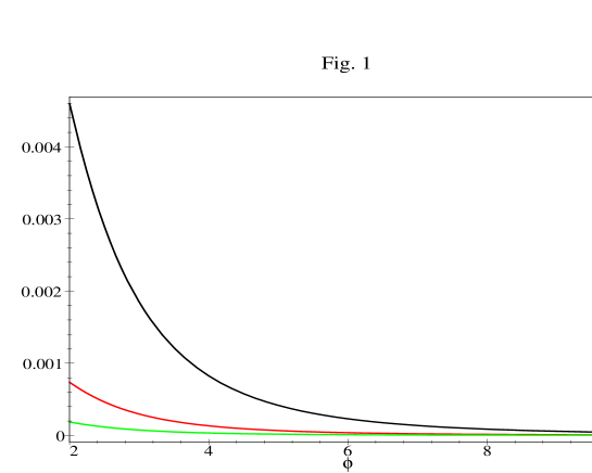
FIG. 1.: Behavior of the radial part of the first WEC inequality, $g_{1}(\phi)$, near the wormhole throat. The curves are, from black to grey, the corresponding to $\alpha=2,5$ and 10 and all them are presented for the case $\phi\th=2$.

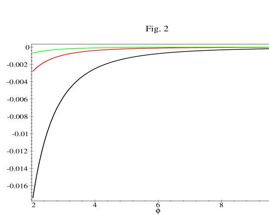
FIG. 2.: As in Fig. 1 but for the function $g_{2}(\phi)$, involved in the second WEC inequality.

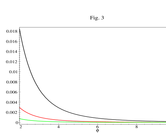
FIG. 3.: As in Fig. 1 but for the function $g_{3}(\phi)$, involved in the third WEC inequality.

REFERENCES

- [1] M. Morris and K. Thorne, Am. J. Phys. 56, 395 (1988)
- [2] M. Morris, K. Thorne and U. Yurtserver, Phys. Rev. Lett. 61, 1446 (1988)
- [3] J. Friedman, M. Morris, I. Novikov, F. Echeverría, G. Klinkhammer, K. Thorne and U. Yurtserver, Phys. Rev. D 42, 1057 (1990)
- [4] V. Frolov and I. Novikov, Phys. Rev. D 42 1913 (1990)
- [5] S. W. Hawking, Phys. Rev. D 46, 603 (1992)
- [6] M. Visser, Nuc. Phys. B328, 203 (1989)
- [7] A. K. Raychaudhuri, Theoretical Cosmology, (Clarendon Press, Oxford, 1979)
- [8] D. Hochberg and M. Visser, gr-qc 9704082.
- [9] A. Agnese and M. La Camera, Phys. Rev. D 51, 2011 (1995)
- [10] L. A. Anchordoqui, S. E. Perez Bergliaffa, D. F. Torres, Phys. Rev. D 55, 5226 (1997)
- [11] D. Hochberg, Phys. Lett. B251, 349 (1990)
- [12] B. Bhawal and S. Kar, Phys. Rev. D 46, 2464 (1992)
- [13] L. A. Anchordoqui, gr-qc 9612056
- [14] T. A. Roman, Phys. Rev. D 47, 1370 (1993)
- [15] S. Kar, Phys. Rev. D 49, 862 (1994)
- [16] S. Kar and D. Sahdev, Phys. Rev. D 53, 722 (1996)
- [17] S. Kar and D. Sahdev, Phys. Rev D 52, 2030 (1995)
- [18] S. D. Maharaj and R. Maartens, J. Math. Phys. 27, 2517 (1986)
- [19] M. Visser, Lorentzian Wormholes (AIP Press, 1996)
- [20] C. W. Misner, K. S. Thorne, and J. A. Wheeler, Gravitation (Freeman, San Francisco, 1973, §32.6)
- [21] J. L. Friedman, K. Schleich, and D. M. Witt, Phys. Rev. Lett. 71, 1486 (1993)