A slightly less grand challenge: Colliding Black Holes using perturbation techniques

Abstract

Perturbation techniques can be used as an alternative to supercomputer calculations in calculating gravitational radiation emitted by colliding black holes, provided the process starts with the black holes close to each other. We give a summary of the method and of the results obtained for various initial configurations, both axisymmetric and without symmetry: Initially static, boosted towards each other, counter-rotating, or boosted at an angle (pseudo-inspiral). Where applicable, we compare the perturbation results with supercomputer calculations.

I Introduction

The grand challenge for supercomputers in numerical relativity is the simulation of the inspiral and merger of two black holes, and the computation of the gravitational radiation emitted in the process. If this event is to be described in full relativistic glory, the use of supercomputers is inevitable. An alternative to this approach is the use of perturbation theory: If the colliding black holes start out so close to each other that they have already formed a common horizon, they can be treated as a linearized perturbation of a single, spherically symmetric black hole, as illustrated in Fig. 1. This method is less complicated and requires considerably less computer resources (CPU time, memory), than the full, non-linear approach. Furthermore, additional analytic insight can be gained which is not accessible in the supercomputer computation.

FIG. 1.: Regarding a close collision of two black holes as a perturbation of the final black hole. Left: Initially static. Right: Initially boosted towards each other, including non-axisymmetric, antiparallel spins.

II The perturbation approach

The full spacetime metric is written as a background metric plus a small perturbation:

$$g_{\mu\nu}=g_{\mu\nu}^{0}+h_{\mu\nu}\;.$$ (1)

We will use the Schwarzschild metric as the background metric $g_{\mu\nu}^{0}$. The field equations are then linearized around the background metric, yielding linear equations for the perturbation.

A Time evolution

The spherical symmetry of the background metric allows the separation of the angular variables, and eventually the reduction of the perturbation equations to a single, one-dimensional wave equation with a potential $V({r_{*}})$ for a scalar function, the Zerilli function $Q({r_{*}})$:

$$\left[{\partial^{2}\over\partial t^{2}}-{\partial^{2}\over\partial{r_{*}}^{2}}+V({r_{*}})\right]Q=0\;.$$ (2)

There is one such Zerilli function for each value of $l$ and $m$, which are the usual parameters in the spherical harmonics used for the angular dependence, and for even and odd parity perturbations. The potential $V({r_{*}})$ (and thus the wave equation) depends on $l$ and the parity, but not on $m$.

B Initial data

In order to obtain initial data for the black hole collision, we use the approach described by Bowen and York [1] solving the constraint equations assuming a conformally flat initial spatial slice:

$$g_{ij}=\phi^{4}\eta_{ij}\;.$$ (3)

Solutions for the conformal factor $\phi$ describing several initially static wormholes were found by Misner [2].

For configurations where the black holes are not static initially, we use the solutions given by Bowen and York [1] for the conformal extrinsic curvature

$$\widehat{K}_{ij} = {3\over 2r^{2}}\left[2P_{(i}n_{j)}-(\eta_{ij}-n_{i}n_{j})P^{c}n_{c}\right]$$ (4)

$$\widehat{K}_{ij} = {3\over r^{3}}\left(\epsilon_{kil}S^{l}n^{k}n_{j}+\epsilon_{kjl}S^{l}n^{k}n_{i}\right)\;,$$ (5)

valid for one black hole with momentum $P$ or spin $S$. The extrinsic curvature for several black holes can be obtained by combining contributions from each black hole.

If the initial configuration is not static, then the conformal factor will be different from its Misner form. However, the difference is of second order in the extrinsic curvature. We can thus ignore the difference, using the Misner form, as long as the extrinsic curvature is not too large.

Initial data for the Zerilli function itself is derived from the initial spatial metric [3], the initial derivative is obtained from the extrinsic curvature [4].

C Radiation emitted

Once the time evolution of all relevant Zerilli functions is known, the total energy radiated as gravitational radiation during the close collision is given by [4]

$$P(r\rightarrow\infty)={1\over 32\pi}\sum_{l,m}\left(\left({\partial\over\partial t}{Q^{\rm even}_{\,lm}}\right)^{2}+\left({Q^{\rm odd}_{\,lm}}\right)^{2}\right)$$ (6)

III Results

A Axisymmetric collisions

The perturbation approach for close collisions was first used by Pullin and Price [3] for two initially static black holes. The results, shown in Fig. 3, indicated excellent agreement with supercomputer calculations for much larger separations than expected. Even at $\mu_{0}$ = 1.36, where a common apparent horizon only begins to form, the difference is less than a factor of 2.

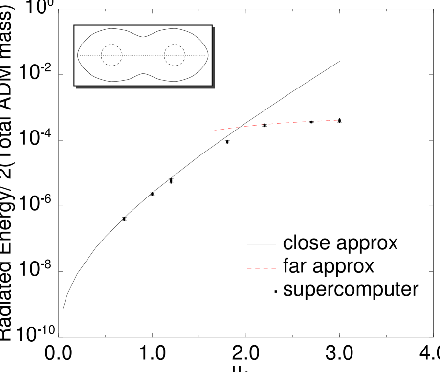
FIG. 2.: Total radiated energy, according to the close approximation, for a collision of two initially static black holes. The parameter $\mu_{0}$ determines the initial separation.

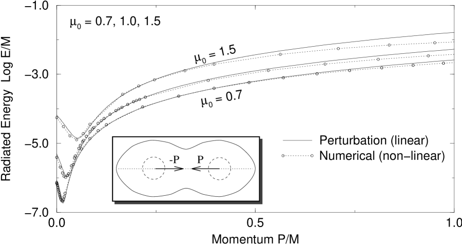
FIG. 3.: Total radiated energy for two black hole initially boosted towards each other.

Figure 3 shows the radiated energy of two black holes initially boosted towards each other [5]. It turns out that the agreement with fully non-linear, numerical calculations also extends to rather large values of the initial momentum. This is again rather unexpected, since the construction of initial data assumed small extrinsic curvature, and thus small initial momentum.

Two counterrotating black holes, with antiparallel spins aligned along the direction of the collision (“Cosmic Screw”), still form an axisymmetric system and result in a final Schwarzschild black hole. The radiated energy as a function of spin is shown in Fig. 5. If both black holes have a spin of $S=\pm 1M^{2}$, the rdaiated energy is incerased by about a factor of $400\dots 1000$ over the non-rotating case.

B Non-axisymmetric collisions

Other than for supercomputer calculations, axisymmetry does not play a major role in the perturbation approach. Two black holes with antiparallel spins, aligned perpendicular to the line of collision, form a simple non-axisymmetric system. It is usually expected that the violation of axisymmetry will increase the amount of radiation. This is not true for this particular situation; rather, the radiation contributed by the spins is lower by a factor of $3/4$, compared to the axisymmetric case.

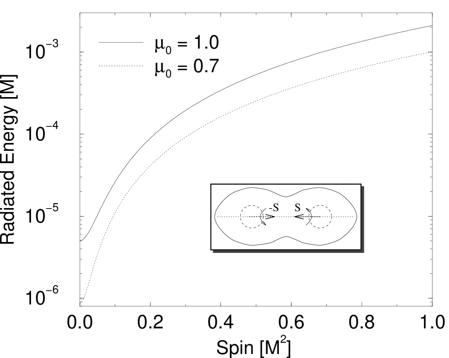
FIG. 4.: Total radiated energy for two black holes carrying antiparallel spins aligned with the direction of collision (“Cosmic Screw”).

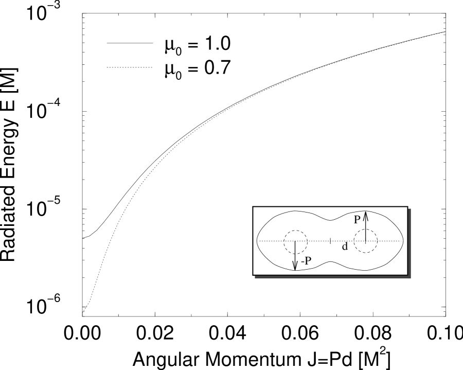
FIG. 5.: Total radiated energy for black hole collisions with the black holes being initially boosted perpendicularly to the line connecting them (“Pseudo-Inspiral”).

Boosting the black holes perpendicularly to the line connecting them also violates axisymmetry. This configuration can be regarded as the start of a collision from a slowly decaying circular orbit. Figure 5 shows the radiated energy as a function of the resulting orbital angular momentum. Since this case results in a rotating black hole, we can only treat it as a perturbation of a Schwarzschild black hole as long as the final angular momentum is small. However, even for $J=0.1M^{2}$, the emitted radiation increases by about two orders of magnitude, compared to the head-on collision.

REFERENCES

- [1] J.M. Bowen and J.W. York, Jr., Phys. Rev. D 21, 2047 (1980)
- [2] C.W. Misner, Ann. Phys. 24, 102 (1963)
- [3] R.H. Price and J. Pullin, Phys. Rev. Lett. 72, 3297 (1994)
- [4] A.M. Abrahams and R.H. Price, Phys. Rev. D 53, 1963 (1996).
- [5] J. Baker et al, Phys. Rev. D 55, 829 (1997).