Quantum Geometry and
Thermal Radiation from Black Holes

Abstract

A quantum mechanical description of black hole states proposed recently within non-perturbative quantum gravity is used to study the emission and absorption spectra of quantum black holes. We assume that the probability distribution of states of the quantum black hole is given by the “area” canonical ensemble, in which the horizon area is used instead of energy, and use Fermi’s golden rule to find the line intensities. For a non-rotating black hole, we study the absorption and emission of s-waves considering a special set of emission lines. To find the line intensities we use an analogy between a microscopic state of the black hole and a state of the gas of atoms.

I Introduction

Progress has recently been made within non-perturbative quantum gravity in understanding how one can describe states of black holes quantum mechanically [1, 2, 3, 4]. In this description the black hole horizon is treated as an interior spacetime boundary where certain boundary conditions, motivated by the geometrical properties of black hole solutions, are imposed. The standard techniques of loop quantum gravity can then be applied, with appropriate modifications required by the presence of the boundary. The degrees of freedom associated with the black hole then turn out to be described by Chern-Simons theory on the boundary (see [1, 2]).

In the present paper we use this description to study emission and absorption processes by quantum black holes. At the outset, we wish to point out our analysis is not complete; at some points we use heuristic arguments and make certain plausible assumptions. However, to some extent our assumptions are supported by the final results.

The description of black hole states proposed within non-perturbative quantum gravity realizes in a rather explicit fashion an old heuristic idea that dates back to early works of Bekenstein (for a recent reference see [5]): a quantum black hole is seen as an ‘atom’ with a lot of internal microstates. A detailed description of these microstates will be given in the following section. However, to motivate certain constructions that follow, let us present a simple heuristic description already at this stage. In non-perturbative quantum gravity spatial quantum geometry, i.e., the quantum geometry “at a given time” is described by the so-called cylindrical states. A cylindrical quantum state is labelled by a graph in space. The edges of this graph have a simple heuristic interpretation of the flux lines of the gravitational field: one can think of the gravitational field (metric tensor) as being concentrated along these edges, similarly as one can think of the usual electric field of Maxwell theory as being concentrated along Faraday’s lines of electric force. A black hole or, more precisely, the black hole horizon “at a given time” is described as a two-surface that may be pierced by the gravitational flux lines. The flux lines excite certain surface degrees of freedom, which are responsible for the black hole entropy (see Fig. 1a).

A black hole state is specified by giving a configuration of the flux lines piercing the horizon, and by describing a quantum state of the surface degrees of freedom. A very convenient basis of quantum states is given by eigenstates of the operator measuring the horizon area. For such an eigenstate each flux line piercing the horizon is labelled by a quantum number: spin $j$. The area comes from intersections of the flux lines with the surface: each flux line intersecting the surface contributes an area proportional to $\sqrt{j(j+1)}$ (see (10)). Let us denote any one of the area eigenstates by ${|\Gamma\rangle}$. States ${|\Gamma\rangle}$ are going to play the key role in what follows. Consider a quantum process in which the black hole jumps from a state ${|\Gamma\rangle}$ to state ${|\Gamma^{\prime}\rangle}$, such that the horizon area changes. This, for example, can be a process in which one of the flux lines piercing the horizon breaks, with one of the ends falling into the black hole and the other escaping to infinity (see Fig. 1b). This is an example of the emission process; the two ends of the flux line can be thought of as the two particle anti-particle quanta in Hawking’s original picture [6] of the black hole evaporation.

           

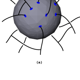
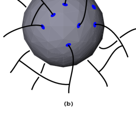
FIG. 1.: (a) The flux lines of gravitational field pierce the black hole horizon and excite curvature degrees of freedom on the surface. The curvature degrees of freedom, described by Chern-Simons theory, account for the black hole entropy in our approach; (b) An example of the emission process in which one of the flux lines breaks, with one of the ends falling into the black hole and the other escaping to infinity.

It is not hard to find the energy of a particle that is emitted. Let us denote by $A(M)$ the dependence of the horizon area of the quantum black hole on its mass $M$ (for simplicity we consider a non-rotating uncharged black hole), and by $\Delta M_{\Gamma\Gamma^{\prime}}$ the change of the black hole mass in the emission process. The quantity $\Delta M_{\Gamma\Gamma^{\prime}}$ should also be equal to the energy of the particle emitted when it reaches infinity. Then for small area changes $\Delta A_{\Gamma\Gamma^{\prime}}$ the energy of the particle emitted is equal to

$$\Delta M_{\Gamma\Gamma^{\prime}}=\left({dA\over dM}\right)^{-1}\,\Delta A_{\Gamma\Gamma^{\prime}}.$$ (1)

For simplicity let us consider the case when the particle emitted is massless. Then its energy $\Delta M_{\Gamma\Gamma^{\prime}}$ is related with its frequency $\omega_{\Gamma\Gamma^{\prime}}$ via Planck’s formula $\Delta M_{\Gamma\Gamma^{\prime}}=\hbar\omega_{\Gamma\Gamma^{\prime}}$. One can also consider the case when the particle emitted carries an angular momentum. Then the angular momentum of the particle is equal to the angular momentum lost by the black hole, and the relation (1) must be modified by replacing the derivative with respect to $M$ by the partial derivative with the black hole angular momentum fixed. Similarly one can consider the emission of charged particles.

As we already mentioned, the spectrum $A[\Gamma]$ of the area is purely discrete in our quantum theory. Thus, the black hole spectrum is discrete: possible transitions $\Gamma\to\Gamma^{\prime}$ correspond to discrete emission lines in the spectrum. However, this by itself does not imply that the black hole spectrum is essentially different from the thermal spectrum predicted by the semiclassical considerations. Indeed, as is argued in [7], quantum fluctuations may smear out the discrete lines in the emission spectrum, which would result in an effectively continuous spectrum. Although the non-commutativity of certain geometrical operators suggests [8] that this is indeed the case in the theory under consideration, this issue is far from being settled. Thus, in this paper, we simply try to find the properties of the discrete emission spectrum, leaving the problem of determining whether the spectrum indeed becomes effectively continuous to further research.

To determine the line intensities and, therefore, the form of the emission spectrum, we, motivated by the “atomic” picture of the black hole, use Fermi’s golden rule. According to this rule, the probability of a transition $\Gamma\to\Gamma^{\prime}$ with a quantum of radiation being emitted is given by

$$W_{\Gamma\to\Gamma^{\prime}}={2\pi\over\hbar}\,|V_{\Gamma\Gamma^{\prime}}|^{2}\,\delta(\omega-\omega_{\Gamma\Gamma^{\prime}}){\omega^{2}d\omega d\Omega\over(2\pi\hbar)^{3}},$$ (2)

where $V_{\Gamma\Gamma^{\prime}}$ is the matrix element of the part of the Hamiltonian of the system that is responsible for the transition. For brevity, we suppress the dependence of this matrix element on initial and final states of the quantum field describing the radiation. Quantity $d\Omega$ in (2) is the element of the solid angle in the direction of the quantum emitted, and $\omega_{\Gamma\Gamma^{\prime}}$ is the frequency of the quantum. We put $c=1$ throughout the paper. The total energy $dI$ emitted by the system per unit time in transitions of this particular type can be obtained by multiplying the above probability by $\hbar\omega$ and by the probability $p(\Gamma)$ to find the system in the initial state ${|\Gamma\rangle}$

$$dI(\Gamma\to\Gamma^{\prime})=\hbar\omega\,p(\Gamma)\,{2\pi\over\hbar}\,|V_{\Gamma\Gamma^{\prime}}|^{2}\,\delta(\omega-\omega_{\Gamma\Gamma^{\prime}}){\omega^{2}d\omega d\Omega\over(2\pi\hbar)^{3}}$$ (3)

Thus, to find the emission spectrum, one has to know the probability distribution $p(\Gamma)$ of the black hole over states ${|\Gamma\rangle}$, and the matrix elements $|V_{\Gamma\Gamma^{\prime}}|$ of the Hamiltonian responsible for transitions. However, as we know from the numerous examples from statistical mechanics, it usually happens that the general form of the spectrum is determined by the probability distribution over states and by such qualitative aspects of the dynamics as selection rules for quantum transitions. Usually only the fine details of the spectrum depend on the precise form of the matrix elements of the Hamiltonian. In this paper we try to learn as much as possible about the black hole emission spectrum without specifying the details of the quantum dynamics, using just the information provided by the kinematics of the theory. As we shall see, it is indeed possible to determine the general form of the spectrum just by knowing the probability distribution $p(\Gamma)$ and by analyzing certain kinematical selection rules.

As the statistical distribution $p(\Gamma)$ we use the one given by the “area” canonical ensemble [9]. Namely, we take the probability $p(\Gamma)$ to find the system in a quantum state $\Gamma$ to be $p(\Gamma)\propto\exp{(-\alpha A[\Gamma])}$, where $A[\Gamma]$ is the “quantum” area of the black hole in the state $\Gamma$, and $\alpha$ is a real positive parameter, playing the role of the quantity conjugate to the area. Some properties of this statistical ensemble are reviewed in the Appendix A. In particular, as we discuss in the appendix, the problem of calculation of the black hole entropy $S$ can be reduced to the problem of calculation of the entropy in this statistical ensemble. It turns out that large black holes correspond to the values of $\alpha$ close to certain critical value $\tilde{\alpha}$. The same critical value $\tilde{\alpha}$ determines the proportionality coefficient between the entropy and the area: $S=\tilde{\alpha}A$. Thus, for large black holes, the relevant values of the parameter $\alpha$ are the ones close to the critical value $\tilde{\alpha}$, and the probability distribution of states is given by:

$$p(\Gamma)\propto e^{-\tilde{\alpha}A[\Gamma]},$$ (4)

where, as we have said above, $\tilde{\alpha}$ coincides with the proportionality coefficient between the entropy and the area $S=\tilde{\alpha}A$. It is clear that this probability distribution is quite natural in the context of black holes. Indeed, (4) simply states that the probability to find the black hole in a state $\Gamma$ is proportional to $\exp{(-S)}$, where $S$ is the entropy of the black hole of the horizon area $A[\Gamma]$. Thus, if one replaces $S$ by the logarithm of the corresponding number $N$ of available states, then (4) becomes the ordinary microcanonical ensemble distribution: $p(\Gamma)\propto 1/N$, in other words, all states $\Gamma$ whose area is close to $A$ have equal probability $1/N$, where $N$ is the total number of such states.

The probability distribution (4) is quite reminiscent of the usual canonical ensemble. Thus, as the standard statistical mechanical argument guarantees that the emission spectrum of any system described by the canonical ensemble is thermal, one could expect the same standard argument to guarantee the thermal character of the emission spectrum in our case. Unfortunately, one cannot refer directly to this argument because the area in used in (4) instead of energy. A minor modification of the argument is necessary in order to make it applicable to the area canonical ensemble. We give such a modified argument in the Appendix B.

Thus, as we show in the appendix, our choice of the probability distribution guarantees that the mean number $n_{\omega lm}$ of emitted quanta in the mode of frequency $\omega$ and angular momentum quantum numbers $l,m$ is given by

$$n_{\omega lm}={\Gamma_{\omega lm}\over e^{\hbar\tilde{\omega}/T}-1},$$ (5)

where

$${1\over T}:=\left({\partial S\over\partial M}\right)_{J}$$ (6)

is the thermodynamical temperature of the black hole,

$$\hbar\tilde{\omega}:=\hbar\omega-\Omega_{H}\hbar m,$$ (7)

$$\Omega_{H}:=T\,\left({\partial S\over\partial J}\right)_{M},$$ (8)

and $\Gamma_{\omega lm}$ is the absorption probability of the black hole in the mode $\omega lm$. To avoid confusion, let us note that the absorption probability is different from the so-called absorption cross-section $\sigma_{abs}$ and is related to the later according to (B5). Thus, with our choice of the probability distribution, the black hole emission spectrum is guaranteed to be thermal in the sense that it has the form (5), independently of details of the microscopic dynamics. Moreover, as we show in the Appendix C, our choice of the probability distribution guarantees the correct ($T^{2}$) dependence of the luminosity of a non-rotating black hole on its temperature. This also holds independently of the black hole microscopics.

Thus, it might seem that all of the properties of the black hole emission spectrum are correctly reproduced as soon as one uses a correct statistical ensemble, and that this holds no matter what is the microscopic description. This conclusion, however, would not be correct. Recall that the ordinary, classical black hole is known to have a very special dependence of the absorption cross-section on the quantum numbers of the particle being absorbed. In particular, $\sigma_{abs}^{(l)}(\omega)$ for a Schwarzschild black hole is very small for large angular momentum $\hbar l$, that is for $l/GM\gg\omega$. Also, for the absorption of the minimal coupled scalar field, the absorption cross-section of s-waves $\sigma_{abs}^{(0)}(\omega)$ is approximately constant and equal to the horizon area for all $\omega$ that matter in (5) (see, for example, [11]). Also, the absorption cross-section $\sigma_{abs}(\omega)$ is a smooth function of the frequency. Only when these (and other) properties are accounted for by a microscopic description can one be satisfied with this description. Thus, details of the microscopic dynamics become important when one studies properties of the black hole absorption cross-section. One could worry, for example, that the quantum mechanical description of the black hole, although giving a thermal emission spectrum in the above sense, does not reproduce correctly the dependence of the absorption coefficient on the quantum numbers $\omega,l$ etc. Also, because the space of states is discrete, one could worry that the absorption properties of the quantum black hole will be similar to those of an atom, that is, that the absorption spectrum will consist of distinct lines. This would correspond to the absorption coefficient very different from the one predicted by the classical theory.

In this paper we make a first step towards investigation of the properties of the black hole absorption cross-section as predicted by the non-perturbative quantum gravity approach. More precisely, we study the emission and absorption of s-waves by a non-rotating, uncharged black hole. In order to be able to use the standard technology from statistical mechanics, we restrict our attention to a special set of lines in the emission spectrum. This allows us to use an analogy between the quantum states of black holes and the states of a gas of atoms. Although our results concern the most uninteresting (however the most dominant in the absorption) case of s-waves, the reader should bear in mind that this paper is a first attempt to study the emission-absorption properties of black holes within the approach of non-perturbative quantum gravity.

The paper is organized as follows. In Sec. II we describe in some details the quantum states of black holes. Sec. III is devoted to the study of the spectrum. We study the emission and absorption of s-waves by considering a special set of lines in the emission spectrum.

II Quantum states

A description of quantum states is now available for various types of non-rotating black holes and it is expected that the main features will be carried over to the rotating case. Let us first describe the quantum states of an uncharged, non-rotating black hole, and then make some comments as to the rotating case. (for details see [1, 2]). Let ${\cal B}$ be the intersection of the black hole horizon with a spatial hypersurface; ${\cal B}$ has the topology of a 2-sphere. A state, in particular, is defined by a set of points $p_{1},\ldots,p_{n}$ on ${\cal B}$ labelled by spins $j_{p}$. In what follows the points on ${\cal B}$ labelled by spins are referred to as punctures. Each set

$${\cal P}=\{j_{p_{1}},\ldots,j_{p_{n}}\}$$

of punctures gives rise to a Hilbert space ${\cal H}_{\cal P}$ of quantum states of the connection on ${\cal B}$, the connection describing the effective black hole degrees of freedom. A black hole state is defined by: (i) a set ${\cal P}$ of punctures on ${\cal B}$; (ii) a vector from the Hilbert space ${\cal H}_{\cal P}$. The dimension of ${\cal H}_{\cal P}$, for a large number of punctures, grows as

$${\rm dim}{\cal H}_{\cal P}\sim\prod_{j_{p}\in{\cal P}}(2j_{p}+1)$$ (9)

The quantum states described are eigenstates of the operator [12] measuring the area of ${\cal B}$. Given a state defined by a set ${\cal P}$ of punctures the corresponding eigenvalue of the area operator is

$$8\pi l_{p}^{2}\gamma\sum_{j_{p}\in{\cal P}}\sqrt{j_{p}(j_{p}+1)},$$ (10)

where $l_{p}$ is the Planck length and $\gamma$ is the so-called Immirzi parameter that arises due to a quantization ambiguity, as is discussed in [13]. Given a black hole with horizon area $A$ one can introduce the statistical mechanical entropy $S$ of the black hole, defined as the logarithm of the number of different quantum states that have an area eigenvalue within the interval of width $l_{p}^{2}$ about $A$. One obtains

$$S={\gamma_{0}\over 4l_{p}^{2}\gamma}\,A,$$ (11)

where $\gamma_{0}$ is a numerical constant $\gamma_{0}\approx 0.12$. As we have mentioned above, the same value for the entropy can be obtained by considering the “area” canonical ensemble, defined by the probability distribution (4) (see the Appendix A for details).

A detailed picture of quantum states for a rotating black hole is not yet available. Thus, we will not treat rotating black holes in the main body of the paper. The only place where rotating black holes are dealt with is the Appendix B, where the thermal character of the emission spectrum from a general rotating charged black hole is discussed. For the purposes of that discussion we shall make here a minor assumption about the rotating black hole states. Namely, we assume that the rotating black hole can be described by quantum states similar to those discussed above, i.e., that among the quantum states describing the black hole, there are ones that are eigenstates of both the area and the angular momentum operators. We assume that the area spectrum is still given by (10), and denote the angular momentum eigenvalues by $J[\Gamma]$. We will not need any further assumptions about these quantum states.

III Spectrum

We restrict our consideration to uncharged, non-rotating black holes, for which a complete microscopic description of states is available, as was described above. This description is used here to deduce some properties of the absorption cross-section for such black holes. Our results also provide a somewhat interesting picture of “atoms” of surface geometry. This section heavily uses the details of the microscopic description of states.

To introduce our main physical idea let us heuristically think of punctures on ${\cal B}$ as “atoms” of surface geometry. According to (10) each atom gives a contribution to the area of ${\cal B}$ that depends on its spin $j_{p}$. Thus, we say that atoms can reside in different quantum states, which are labelled by the quantum number $j_{p}$. Then, just as real atoms can jump from one excited state to another emitting quanta of radiation, our atoms can undergo transitions in which spin $j_{p}$ changes, thus changing the horizon surface area of black hole and emitting radiation.

We assume that in the process of evolution described by an appropriate Hamiltonian operator, individual atoms jump from one quantum state to another, and the line intensities are given by Fermi’s formula. We consider here only emission processes involving just a single atom; as we shall see, this simplifies the whole discussion considerably. Note, however, that in this way we will be able to analyze only a part of the emission spectrum. To get the complete spectrum one should consider processes involving simultaneously any number of atoms. We believe, however, that the results we obtain for this simplified case give one an important insight on what can be expected in the more general situation. Indeed, on general grounds one might expect that transitions involving simultaneously more than one puncture are much less probable and that, therefore, the transitions we consider here determine the form of the spectrum.

The probability of a transition involving just a single atom is then given by the expression (2), with $\hat{V}$ being a part of the quantum Hamiltonian responsible for the transitions of this type. The intensity of a line is given by (3), with the labels $\Gamma,\Gamma^{\prime}$ of the initial and final states being replaced by initial and final spins $j,j^{\prime}$ of the atom involved in the transition. Since the final state is $(2j^{\prime}+1)$ degenerate, one should also multiply the intensity (3) by the degeneracy. Because we are using the analogy between a state of the black hole and a state of the gas of atoms, it is natural to replace the probability $p(\Gamma)$ in (2), (3) by the number $n_{j}$ of atoms in the initial state $\Gamma$ that are in one and the same state $j$. The function $n_{j}(A)$, which gives the number $n_{j}$ of “atoms” excited to the level $j$ among all the “atoms” that compose a black hole of given area $A$, is introduced, and its properties are discussed in the Appendix A. This function is analogous to the occupation number in the statistical mechanical treatment of the harmonic oscilator. Similarly to the case of the harmonic oscilator, the thermal character of radiation in our case comes from the properties of the function $n_{j}(A)$.

In the simplest case of the absorption of s-waves, the final state of the field describing the radiation is spherically symmetric. Thus, one can integrate out the angular dependence in (3). Let us denote the corresponding integral of the squared absolute value of the transition matrix element by $\Phi_{jj^{\prime}}$. Let us also absorb in $\Phi$ all constant unimportant factors. To get rid of the $\delta$-function in (3) one integrates over $d\omega$. Thus, the intensity of the line $j\to j^{\prime}$ becomes

$$I(j\to j^{\prime}) = \omega_{jj^{\prime}}^{3}\,n_{j}(A)\,\Phi_{jj^{\prime}}\,(2j^{\prime}+1),$$ (12)

$$\hbar\omega_{jj^{\prime}} = \left({dM\over dA}\right)\,(A_{j}-A_{j^{\prime}}).$$ (13)

Note that we have multiplied the whole expression by $2j^{\prime}+1$, which is the degeneracy of the final state. The latter formula is what one obtains from (1) considering transitions that change only one puncture. Here $A_{j}=8\pi l_{p}^{2}\gamma\sqrt{j(j+1)}$.

The expression (12) is the desired formula for the emission line intensity. Knowing the matrix elements of the transition Hamiltonian one could immediately calculate the intensities of all the lines in the emission spectrum. It is interesting, however, that some information about the overall form of the spectrum can be obtained even without knowing the Hamiltonian.

We are interested in getting the spectrum of a large black hole, that is a black hole whose horizon area is large in Planck units. As we discuss in the Appendix A, most of the area of a large black hole is due to the contribution from atoms whose spin $j=1/2$. This is, for example, manifested by the fact that $n_{1/2}(A)\to\infty$ as $A\to\infty$, while all other occupation numbers $n_{j}$ remain finite. An implication of this fact for the emission-absorption spectrum is that the lines corresponding to transitions to and from $j=1/2$ are most intensive, for a large black hole by far more intensive then any other lines. For emission spectrum, for example, this would mean that there is effectively only one intense emission line $1/2\to 0$, and all other lines are of negligible intensity as compared with this one. Of course, such a spectrum is very far from thermal one. Note that this would not be in a contradiction with the general result (B7). Indeed, the spectrum in this case is still of the form (B7), but the absorption coefficient is distributional and picked at a single frequency.

It turns out, however, that the line $1/2\to 0$ is forbidden by selection rules. And, as we shall see, with this line removed from the spectrum, the remaining lines form a spectrum close to thermal. The selection rule forbidding the line $1/2\to 0$ is independent of the details of the Hamiltonian describing the system. It arises because of the requirement of gauge invariance. As we have said above, a quantum state of black hole is described by a collection of spins labelling the punctures and by a state of Chern-Simons theory on the punctured horizon surface. For state of Chern-Simons theory to exist, one condition should be satisfied by the spins labelling the punctures. Namely, the decomposition into irreducible representations of the tensor product of representations labelling the punctures should contain the trivial representation. In fact, the multiplicity of the trivial representation is exactly the dimension (9) of the Hilbert space of Chern-Simons theory. Translated on the language of spins labelling the punctures, this condition states that the (algebraic) sum of all spins should be an integer. Only such configurations of spins correspond to black hole states. Let us now return to the transition $1/2\to 0$. If the initial state of the black hole is such that the sum of all spins gives an integer, then the state obtained after this transition does not satisfy this condition. Thus, the transition $1/2\to 0$ should be forbidden.

Since the transitions from $j=1/2\to j=0$ are forbidden, we have to deal only with with $j=1$ and higher. For these values of spins $j$ the expression for $n_{j}(A)$ simplifies. Indeed, as we discuss in the Appendix A, large black holes correspond to values of $\alpha$ very close to $\tilde{\alpha}$, the later being the proportionality coefficient between the entropy and the area. Thus, for $j>1/2$, the occupation number $n_{j}$ in the limit of large $A$ becomes independent of the area and approximately equal to $n_{j}(\tilde{\alpha})$. It is not hard to find its asymptotic behavior for large $j$:

$$n_{j}\propto je^{-\tilde{\alpha}A_{j}}.$$ (14)

Note that this is a function of $j$ only.

After these preliminaries, we can begin the discussion of properties of the spectrum. To find the emission spectrum $I(\omega)$ one has to find the energy $I$ emitted per frequency interval as a function of frequency $\omega$. Let us note that the relations (12), (13) have the form

$$I(j\to j^{\prime})=\omega^{3}_{jj^{\prime}}f_{1}(j,j^{\prime})$$ (15)

$${\hbar\omega_{jj^{\prime}}\over T}=f_{2}(j,j^{\prime}),$$ (16)

where $f_{1}(j,j^{\prime})=n_{j}\Phi_{jj^{\prime}}(2j^{\prime}+1),f_{2}=\tilde{\alpha}(A_{j}-A_{j^{\prime}})$ are functions of $j,j^{\prime}$ only. Here $T$ is the thermodynamical temperature of the black hole (6). To find the total intensity $I(\omega)$ of the radiation emitted as a function of frequency, one has to divide the frequency range of interest into small intervals, and sum the intensities of all lines that belong to each particular interval. Then the relations (15), (16) can be thought of as giving the parametric dependence of $I$ on $\hbar\omega/T$ (the parameters being $j,j^{\prime}$). Thus, we find that $I(\omega)$ depends on the frequency $\omega$ only in the combination $\hbar\omega/T$

$$I=I(\hbar\omega/T).$$

It is not hard to find the properties of this function in the two limiting cases $\hbar\omega/T\to 0,\hbar\omega/T\to\infty$. Indeed, the presence of $\omega^{3}$ in (15) guarantees that $I\to 0$ as $\hbar\omega/T\to 0$. On the other hand, one can use the asymptotics (14) of $n_{j}$ to determine the behavior of $I$ for large frequencies. Indeed, the most intensive line with frequency $\omega$ (for large $\hbar\omega/T$) is the one corresponding to the transition $j(\omega)\to 0$, where

$$\hbar\omega/T=\tilde{\alpha}A_{j(\omega)}.$$

The intensity of this line is proportional to $\exp{-\tilde{\alpha}A_{j(\omega)}}=\exp{-\hbar\omega/T}$. The other, less intensive lines with the same frequency correspond to transitions $j(\omega)+k\to k$; their intensity is $\exp{-\tilde{\alpha}A_{k}}$ less. Summing the intensities of all these lines, one gets the asymptotics of the emission intensity for large frequencies:

$$I(\omega)\propto\exp{\left(-\,{\hbar\omega\over T}\right)},$$ (17)

where $T$ is the thermodynamical temperature (6) of the black hole. In other words, we find that the emission spectrum $I(\omega)$ behaves at high frequencies as the Planck thermal spectrum of the temperature $T$.

Of course, it is not surprising that we found some properties of the thermal spectrum. Indeed, recall that the general results of the Appendix guarantee that the intensity $I$ of the radiation emitted in s-waves must have the form

$$I(\omega)d\omega\sim{\omega^{3}\sigma_{abs}^{(0)}(\hbar\omega/T)d\omega\over e^{\hbar\omega/T}-1},$$ (18)

where the absorption cross-section $\sigma_{abs}^{(0)}$ is a function of $\hbar\omega/T$. Thus, the behavior of $I$ for large and small frequencies that we have demonstrated above could have been derived directly from the general result (18). However, the analysis we just presented allows one to learn more about the emission spectrum then just its general form (18). Note that (18) still does not guarantee that the emission spectrum is close to that of a black hole. It can still happen that the absorption $\sigma_{abs}$ is very different from the one predicted by the classical theory. Indeed, from the classical theory we know that $\sigma_{abs}^{(0)}(\omega)$ is approximately constant for frequencies that matter in (18). It could happen that the absorption cross-section predicted by the quantum theory is different.

To test the dependence of $\sigma_{abs}^{(0)}$ on $\omega$, we present a result of calculation performed with formula (12). We choose transition matrix elements in the simplest possible way. Namely, we take $V_{jj^{\prime}}$ to be independent of $jj^{\prime}$, and assume that no transitions to the state $j=0$ are allowed, thus treating the state $j=1/2$ as the ‘ground’ state. In particular, this automatically takes into account the selection rule that forbids the transitions $j=1/2\to j=0$. The corresponding spectrum is shown in FIG. 2. The first plot shows lines with their intensities computed via (12). Each line is shown as an impulse at a point on the $\hbar\omega/T$ axis. The height of an impulse represents the intensity of the line. We are interested in line intensities only up to an overall multiplicative factor; thus, no units are shown on the $y$-axis. The second plot shows the total intensity $I(\omega)$ as a function of frequency. To get $I(\omega)$ here we divided the frequency range into small intervals and added the intensities of all the lines belonging to the same interval. Although the emission occurs only at certain frequencies, the enveloping curve of the spectrum is perfectly thermal, as is clear from the second plot. This means that, although the absorption coefficient is distributional, its non-zero value is approximately constant for the whole range of frequencies, in agreement with the classical theory. Note that the total intensity decreases exponentially as $\exp{(-\hbar\omega/T)}$ (second plot), in accordance with our conclusion above. The notable fine structure of emission lines (first plot) also deserves attention. Thus, to the extent the naive model described is correct, the properties of the absorption cross-section reproduce those of the classical black hole. It would be much more interesting, however, to try to compute the absorption cross-section of s-waves exactly and compare it with the classical expression (the horizon area). We hope to perform a calculation to this effect in the future.

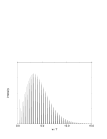
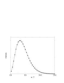
FIG. 2.: Emission lines with their intensities (above) and the total intensity of the radiation emitted per frequency interval as a function of frequency (below).

Several comments are in order. (i) It is instructive to compare the results we have obtained with the results of Bekenstein and Mukhanov [5]. Using a simple model of quantum states of the black hole they found that the emission spectrum consists of discrete lines with the intensity of high frequency lines exponentially damped as in the thermal spectrum. Their model also predicted that the smallest frequency emission line is approximately the one with the largest intensity, thus the spectrum being very different in form from the thermal one. In contrast, the spectrum we have found is much closer in form to the thermal spectrum. (ii) Let us compare our results with the results on the black hole emission-absorption spectra obtained using the microscopic description based on D-branes [14]. The two descriptions are similar in the sense that both describe black holes as composed of some elementary fundamental building blocks: the flux lines of gravitational field as “atoms” of geometry in our picture, and D-branes in the string picture. In both cases thermality is a result of averaging over a large number of microscopic states. Thus, our approach gives the same answer to the question of information loss as string theory. There are important differences, however. Unlike the case of string theory, our description is not sypersymmetric and works entirely in four spacetime dimensions. Because of this, the black holes whose description is still problematic in string theory, such as non-rotating, uncharged black holes in four dimensions, are the ones that are easiest to describe in our framework. Also, our approach is more geometric, the black hole degrees of freedom “live” in our approach on the black hole horizon. Thus our approach directly accounts for the black hole entropy as being proportional to the area. In string theory description, it is harder to see “where” the degrees of freedom of the black hole “live”, and the area of the horizon plays no role, the black hole entropy being thought of as a function of mass and other charges. Thus, the two approaches are complimentary more than contradicting. We must admit, however, that the string description of black holes gives results that precisely agree with the results that follow from semi-classical considerations. The results of our approach are so far more modest, the agreement with the semi-classical results being reached only at a qualitative level. (iii) Although we have found that the spectrum is discrete, it may be the case that the discrete lines in the emission spectrum get smeared out by quantum fluctuations, as it was argued for in [7, 8]. Thus, our results by themselves do not imply that the black hole spectrum in loop quantum gravity is discrete. Further work is necessary to understand implications of the quantum fluctuations of the black hole horizon for the emission spectrum. (iv) One has to keep in mind that only the transitions involving one atom were considered. It is known [15, 16] that one obtains a quasi-continuous spectrum considering transitions involving an arbitrary number of punctures. Thus, another possibility is that the discrete spectrum we have found is only a part of a complete quasi-continuous emission spectrum of the quantum black hole. It might be, however, that the transitions involving simultaneously many atoms are highly suppressed (or forbidden) as compared with the one-atom transitions. Thus, the dynamics of the theory may be such that the lines analyzed in this paper are the most intensive ones, determining the form of the emission spectrum. However, certainly a more quantitative argument in support of this is necessary.

A Area canonical ensemble

In this appendix we introduce the ‘area’ canonical ensemble [9] and discuss some of its properties. Let us introduce a parameter $\alpha$, which will be referred to as the intensive parameter conjugate to the area, and consider the following function of $\alpha$, the statistical sum

$$Q(\alpha)=\sum_{\Gamma}e^{-\alpha A[\Gamma]}.$$ (A1)

Thus, this is a Gibbs-type statistical ensemble; however, the area is used instead of energy. Knowing the statistical sum $Q(\alpha)$ as a function of intensive parameter one can find all other thermodynamical functions using the standard thermodynamical relations. In particular, the dependence $S(A)$ of the entropy on the area can be deduced from the dependence of the expectation value of the area $A(\alpha)$ and the entropy $S(\alpha)$ on the parameter $\alpha$:

$$A(\alpha)=\sum_{\Gamma}A[\Gamma]p[\Gamma]=-{d\ln{Q}\over d\alpha},$$ (A2)

$$S(\alpha)=\sum_{\Gamma}p[\Gamma]\ln{p[\Gamma]}=\alpha A(\alpha)+\ln{Q(\alpha)},$$ (A3)

where

$$p[\Gamma]={1\over Q}e^{-\alpha A[\Gamma]}.$$ (A4)

This then gives a parametric dependence of $S$ on $A$.

In the particular case of the states $\Gamma$ given by those described in the Sec. II, the statistical sum $Q(\alpha)$ can be easily calculated:

$$Q(\alpha)=\prod_{j}{1\over 1-(2j+1)e^{-\alpha A_{j}}},$$ (A5)

where $A_{j}=8\pi l_{p}^{2}\gamma\sqrt{j(j+1)}$. The factors of $(2j+1)$ appear here because each “atom” state is $(2j+1)$ degenerate. One can then find the following expression for the mean value $A(\alpha)$

$$A(\alpha)=\sum_{j=1/2}^{\infty}\,A_{j}\,n_{j}(\alpha),$$ (A6)

where $n_{j}(\alpha)$ is given by

$$n_{j}(\alpha)={(2j+1)e^{-\alpha A_{j}}\over 1-(2j+1)e^{-\alpha A_{j}}}.$$ (A7)

This function plays an important role in our discussion of the properties of the emission spectrum in Sec. III. It is easy to see that each function $n_{j}(\alpha)$ plays the role of the mean number of punctures that have the spin $j$. According to (A2), $\alpha$ controls the mean value of the black hole area. Thus, one can use $A$ instead of $\alpha$ as the argument of $n_{j}$. The function $n_{j}(\alpha(A))$ then, given the black hole horizon area, tells how many there are atoms excited to the level $j$ among all the atoms that compose the black hole.

Some interesting properties of the “area” canonical ensemble can be derived from the properties of $n_{j}$. Note that $n_{j}(\alpha)$ is finite for all $j$ for sufficiently large $\alpha$. However, as $\alpha$ decreases, which corresponds to the increase in the “temperature” in this ensemble, for the value $\tilde{\alpha}=\ln{2}/A_{1/2}$ of $\alpha$ the denominator of $n_{1/2}(\alpha)$ becomes zero. Thus, as $\alpha$ approaches the value $\tilde{\alpha}$, the occupation number $n_{1/2}\to\infty$, with all other occupation numbers remaining finite. Correspondingly, the physical quantities such as the area and entropy diverge in the limit $\alpha\to\tilde{\alpha}$. Formally, this corresponds to a phase transition in our statistical ensemble. The reason for this phase transition is the fact that density of states grows linearly with the area. Indeed, it is not hard to show that the phase transition of the type described occurs in the “area” statistical ensemble if and only if the density of states grows exponentially with the area. An analogous phase transition is known to occur for ordinary statistical systems described by the Gibbs ensemble, for which the density of states grows exponentially with the energy. Thus, the fact that the physical quantities such as $A,S$ become large as $\alpha$ approaches the critical value $\tilde{\alpha}$ imply the linear dependence of the entropy on the area for large areas: $S=\tilde{\alpha}A$. The same expression for the entropy can be obtained by a simple counting of states. This supports the validity of the usage of the “area” canonical ensemble. Let us also note that, because $n_{1/2}\to\infty$ as $A\to\infty$, for large areas most of the “atoms” in the ensemble are in the state with $j=1/2$. This last fact is important in our discussion of the properties of the spectrum in Sec. III.

Several comments are in order. (i) It is interesting to note that, while the usual energy canonical ensemble is not applicable to description of black holes, the “area” canonical ensemble is. We do not know whether there is any deep physical significance behind this fact. It might simply be that the “area” canonical ensemble is a relevant description for systems whose density of states grows linearly with the area. Note, however, that the probability distribution $p[\Gamma]$ given by the “area” canonical ensemble is also consistent with the properties of the black hole radiation. Indeed, as is shown in the next Appendix, this probability distribution guarantees the correct thermal properties of the black hole emission spectrum. Thus, the ensemble in which “energy squared” (area) is used instead of energy, which is quite a bizarre ensemble from the point of view of ordinary statistical mechanics, appears to be very suited for a description of black holes. (ii) Let us comment on a relation between the above “area” ensemble description of black holes and the path integral description [17]. In the later approach, the statistical sum of a gravity system is found by summing (integrating) over Euclidean field configurations weighted with $\exp{(-S)}$, where $S$ the Euclidean action functional evaluated on the corresponding field configuration. The field configurations that matter most in this path integral are given by the solutions of the classical field equations. In the context of asymptotically flat spacetimes, the “bulk” part of the action vanishes on the solutions, and the only contribution to the action comes from the boundary term. When evaluated on field configurations corresponding to Euclidean black holes, the boundary term renders always the value $A/4l_{p}^{2}$, where $A$ is the black hole horizon area. This then results in the black hole entropy equal to $A/4l_{p}^{2}$. It might seem, that our prescription (A4) for the black hole statistical ensemble is inconsistent with the path integral approach, in which the statistical weight of any black hole spacetime is also given by $\exp{-\alpha A}$, but the parameter $\alpha$ is set to the constant value $1/4l_{p}^{2}$ and not allowed to vary. Note, however, that for large black holes, as we discussed above, the value of $\alpha$ in the “area” canonical ensemble is very close to the value $\tilde{\alpha}$. In fact, $|\alpha-\tilde{\alpha}|\sim l_{p}^{2}/A$. But the value $\tilde{\alpha}$ is just the proportionality coefficient between the entropy and the area. Thus, for large black holes, the “area” canonical ensemble statistical distribution effectively reproduces the one of the path integral approach. In other words, for black holes that are large in Planck units, there is no inconsistency between the two approaches. This is the best one can expect: the two prescriptions agree in their domain of applicability. Indeed, the semiclassical path integral approach can only be trusted for large black holes, as well as the statistical mechanical description based on the “area” ensemble is applicable only to sufficiently complicated systems with a large number of internal states.

B Thermal character of the spectrum

In this appendix we show that, if the probability distribution of quantum states of the black hole is given by (4), then the spontaneous emission spectrum is thermal in the sense that it has the form (5). We use the standard thermodynamical argument, which states that the emission spectrum of a system described by the canonical ensemble is thermal. However, in the case of black holes, we cannot refer to that argument directly because area is used instead of energy in (4). Our argument is somewhat similar to the one given in [18].

Let us introduce the so-called Einstein coefficients. We denote by $A_{\omega lm}$ the coefficient of spontaneous emission in the mode $\omega lm$. It is defined so that the mean population $n_{\omega lm}$ of this mode due to spontaneous emission is exactly $A_{\omega lm}$. We denote by $B^{\uparrow}_{\omega lm}$ the Einstein coefficient of stimulated emission. It is defined in such a way that, if the number of incoming quanta in the mode $\omega lm$ is $k_{\omega lm}$, then the population of this mode in the out-going radiation due to stimulated emission is $B^{\uparrow}_{\omega lm}k_{\omega lm}$. We denote by $B^{\downarrow}_{\omega lm}$ the Einstein coefficient of absorption. It is defined in such a way that, if the number of incoming quanta in the mode $\omega lm$ is $k_{\omega lm}$, then the fraction $B^{\downarrow}_{\omega lm}k_{\omega lm}$ of this mode is absorbed by the system. For brevity, we will sometimes suppress the dependence of these coefficients on $\omega,l,m$.

We will first show that there exists a relation between the coefficients $B^{\downarrow},B^{\uparrow}$. One can write the following expressions for the ratio of these coefficients

$${B^{\uparrow}\over B^{\downarrow}}={\sum_{\Gamma,\Gamma^{\prime}}p(\Gamma^{\prime})W_{\Gamma^{\prime}\to\Gamma}\over\sum_{\Gamma,\Gamma^{\prime}}p(\Gamma)W_{\Gamma\to\Gamma^{\prime}}},$$ (B1)

where both sums are taken over $\Gamma,\Gamma^{\prime}$ subject to the conditions $\omega_{\Gamma^{\prime}\Gamma}=\omega>0,\Delta J_{\Gamma^{\prime}\Gamma}=\hbar m$, and where $p(\Gamma)$ is the probability (4). Now note that

$$p(\Gamma)=e^{\tilde{\alpha}A[\Gamma^{\prime}]-\tilde{\alpha}A[\Gamma]}\,p(\Gamma^{\prime})=e^{{1\over T}(\hbar\omega_{\Gamma^{\prime}\Gamma}-\Omega_{H}\Delta J_{\Gamma^{\prime}\Gamma})}\,p(\Gamma^{\prime})=e^{\hbar\tilde{\omega}/T}\,p(\Gamma^{\prime}),$$ (B2)

where the definitions (6), (8) were used to write the second and third identity. Thus, we have

$$B^{\downarrow}=e^{\hbar\tilde{\omega}/T}\,B^{\uparrow},$$ (B3)

where we have used the fact that $W_{\Gamma^{\prime}\to\Gamma}=W_{\Gamma\to\Gamma^{\prime}}$.

We can now relate the coefficients $B$ with the absorption probability $\Gamma$. The fraction of incoming radiation that is absorbed by the black hole consists of two parts: the part that is absorbed minus the part emitted in the processes of stimulated emission. Thus, we have for the absorption probability

$$\Gamma=B^{\downarrow}-B^{\uparrow}.$$ (B4)

Note that the absorption probability $\Gamma$ is different from the so-called absorption cross-section $\sigma_{abs}$. The two are, however, related according to:

$$\sigma_{abs}(\omega)=\sum_{l}\sigma_{abs}^{(l)}(\omega){\pi\over\omega^{2}}\sum_{l=0}^{\infty}\sum_{m}\Gamma_{\omega lm},$$ (B5)

where we have also introduced the so-called partial absorption cross-sections $\sigma_{abs}^{(l)}$.

Let us now discuss a relation between the coefficients $A,B^{\uparrow}$, which are not independent. Let us assume that the interaction of the black hole with the field describing the radiation quanta is linear, as it is the case, for example, for the interaction of an atom with electromagnetic radiation. In this case one can use the standard formulas for the matrix elements of the creation and annihilation operators to conclude that the probability of emission of a quantum in a mode in which there are already $k$ quanta is given by $k+1$ times the probability of spontaneous emission in the same mode. This yields

$$A=B^{\uparrow}.$$ (B6)

Now, using the relations (B3)-(B6), we can conclude:

$$n_{\omega lm}=A_{\omega lm}={\Gamma_{\omega lm}\over e^{\hbar\tilde{\omega}/T}-1},$$ (B7)

which is the well-known expression for the black hole radiation spectrum.

The above argument is very general. To prove (B7) we have used only the assumption that the distribution of states is given by (4), and the relation (B6) that holds for a large class of interaction Hamiltonians. This means that the thermal character of radiation from the quantum black hole is independent on the details of microscopic description as well as on the details of the quantum dynamics. It depends only on the form of the probability distribution describing the black hole.

C Luminosity

In this appendix we restrict our attention to uncharged non-rotating black holes, and study the dependence of the total luminosity of the quantum black hole on its temperature. For a classical black hole, the emission is dominated by s-waves, for which the absorption cross-section is approximately equal to the horizon area (see, e.g. [19]). This gives the luminosity proportional to the squared black hole temperature. However, we cannot refer to this argument for the case of a quantum black hole, because no such property of the absorption cross-section in the quantum theory was established. Thus, we give a different, applicable to a quantum black hole argument to the same effect.

The total luminosity is defined as amount of energy lost by the black hole per unit time. We show that the dependence of this on the black hole temperature is

$${dM\over dt}\sim T^{2}.$$ (C1)

As in the previous subsection, we find that this result is very general, that is, it is independent on the black hole microscopics. Also, as above, we consider only the emission due to massless quanta.

For the rate with which the black hole looses its mass one has

$${dM\over dt}=\sum_{lm}\int_{0}^{\infty}{d\omega\over 2\pi}\hbar\omega{\Gamma_{\omega lm}\over e^{\hbar\omega/T}-1},$$ (C2)

where we used the fact that the black hole is non-rotating $\Omega_{H}=0$. Our key observation is that we get (C1) given that $\Gamma_{\omega lm}$ depends on $\omega$ only in the combination $\hbar\omega/T$. Indeed, in this case we can introduce the new integration variable $\hbar\omega/T$. Then (C2) is given by $T^{2}$ times the expression that does not depend on the temperature anymore. Assuming that the luminosity is finite, we get (C1). Note that this result will hold even if the absorption cross-section $\sigma$ is distributional, which we can expect for a black hole with a discrete spectrum.

For a Schwarzschild black hole the absorption probability $\Gamma$ is given by a relation similar to (B4)

$$\Gamma=B^{\downarrow}-B^{\uparrow}\sim\sum_{\Gamma,\Gamma^{\prime}}\left[p(\Gamma^{\prime})W_{\Gamma^{\prime}\to\Gamma}-p(\Gamma)W_{\Gamma\to\Gamma^{\prime}}\right],$$ (C3)

where the sum is taken over $\Gamma,\Gamma^{\prime}:\omega_{\Gamma^{\prime}\Gamma}=\omega$. Let us note now that terms in the sum in (C3) depend solely on the quantum numbers labelling $\Gamma,\Gamma^{\prime}$: there is no dependence on the temperature of the black hole. The only place where the dependence on the temperature comes into play is the condition $\omega_{\Gamma^{\prime}\Gamma}=\omega$. To see this, let us rewrite this condition in terms of $\Delta A_{\Gamma\Gamma^{\prime}}$. Using (1) we get

$$\hbar\omega=\hbar\omega_{\Gamma^{\prime}\Gamma}={dM\over dA}\,\Delta A_{\Gamma\Gamma^{\prime}}=\tilde{\alpha}\,T\,\Delta A_{\Gamma\Gamma^{\prime}},$$ (C4)

where we have used the definition of $T$ (6) and the fact that $S=\tilde{\alpha}A$. Thus, the condition on states $\Gamma,\Gamma^{\prime}$ involves $\omega$ only in the combination $\omega/T$. This simple observation proves the property (C1).

REFERENCES

- [1] K. Krasnov, On statistical mechanics of Schwarzschild black holes, Gen. Rel. and Grav. 30, No. 1, 53-68 (1998).
- [2] A. Ashtekar, J. Baez, A. Corichi, K. Krasnov, Quantum geometry and black hole entropy, Phys. Rev. Lett. 80, No. 5, 904-907 (1998).
- [3] A. Ashtekar, A. Corichi, K. Krasnov, Black hole sector of the classical phase space, CGPG preprint.
- [4] A. Ashtekar, J. Baez, K. Krasnov, Quantum geometry of black hole horizons, CGPG preprint.
- [5] J. Bekenstein, V. Mukhanov, Spectroscopy of the quantum black hole, Phys. Lett. B360, 7 (1995).
- [6] S. Hawking, Particle creation by black holes, Commun. Math. Phys. 43, 212 (1975).
- [7] J. Mäkelä, Black hole spectrum: continuous or discrete?, available as gr-qc/9609001.
- [8] K. Krasnov, Area spectrum in quantum gravity, Class. Quant. Grav., in press.
- [9] K. Krasnov, Geometrical entropy from loop quantum gravity, Phys. Rev. D55 3505 (1997).
- [10] J. D. Bekenstein, Statistical black hole thermodynamics, Phys. Rev. D12, No. 10, 3077-3085 (1975); S. W. Hawking, Black holes and thermodynamics, Phys. Rev. D13, No. 2, 191-197 (1976).
- [11] S. Giddings, Quantum mechanics of black holes, Lectures given at Summer School in High Energy Physics and Cosmology, Trieste, Italy, 1994, Published in Trieste HEP Cosmology 1994: 530-574.
- [12] C. Rovelli and L. Smolin, Discreteness of area and volume in quantum gravity, Nucl. Phys. B442, 593 (1995); Erratum: Nucl. Phys. B456, 734 (1995). R. De Pietri and C. Rovelli, Geometry eigenvalues and scalar product from recoupling theory in loop quantum gravity, Phys. Rev. D54, 2664 (1996). A. Ashtekar, J. Lewandowski, Quantum theory of geometry I: Area operators, Class. Quant. Grav. 14, 55 (1997). K. Krasnov, On the constant that fixes the area spectrum in canonical quantum gravity, Class. Quant. Grav. 15, L1-L4 (1998).
- [13] G. Immirzi, Quantum gravity and Regge calculus, Nucl. Phys. Proc. Suppl. 57 65-72 (1997). C. Rovelli and T. Thiemann, The Immirzi parameter in quantum general relativity, Phys. Rev. D57 1009-1014 (1998).
- [14] S. R. Das and S. D. Mathur, Comparing decay rates for black holes and D-branes, Nucl. Phys. B478, 561-576 (1996); J. Maldacena and A. Strominger, Black hole greybody factors and D-brane spectroscopy, Phys. Rev. D55, 861-870 (1997).
- [15] M. Barreira, M. Carfora, C. Rovelli, Physics with non-perturbative quantum gravity: radiation from a quantum black hole, Gen. Rel. and Grav. 28, 1293-1299 (1996).
- [16] C. Rovelli, Loop quantum gravity and black hole physics, Helv. Phys. Acta., 69, 582 (1996).
- [17] G. Gibbons and S. Hawking, Action integrals and partition functions in quantum gravity, Phys. Rev. D15, 2752-2756 (1977); J. D. Brown and J. W. York, Microcanonical functional integral for the gravitional field, Phys. Rev. D47, No. 4, 1420-1431 (1993).
- [18] J. D. Bekenstein and A. Meisels, Einstein A and B coefficients for a black hole, Phys. Rev. D15, 2775-2781 (1977).
- [19] D. Page, Particle emission rates from a black hole: Massless particles from an uncharged, non-rotating black hole, Phys. Rev. D13, No. 2, 198 (1976).