[

Gravitational wave extraction and outer boundary conditions by perturbative matching

Abstract

We present a method for extracting gravitational radiation from a three-dimensional numerical relativity simulation and, using the extracted data, to provide outer boundary conditions. The method treats dynamical gravitational variables as nonspherical perturbations of Schwarzschild geometry. We discuss a code which implements this method and present results of tests which have been performed with a three dimensional numerical relativity code.

]

Numerical relativity represents the only currently viable method for obtaining solutions to Einstein equations for highly dynamical and strong field sources of gravitational radiation. Using these techniques to study coalescing black hole binaries is the purpose of the multi-institutional Binary Black Hole “Grand Challenge” Alliance effort[1] which is presently underway in the United States. This effort is also motivated by the prospect of observations with the next generation of gravitational wave detectors.

In addition to tremendous demands on computational resources, implementing the standard $3+1$ [2, 3] formulation of Einstein theory as a Cauchy problem [4] is complicated considerably by the necessity of imposing boundary conditions which maintain numerical accuracy and the physical correctness of the solution. Both inner and outer boundary conditions have received considerable attention. Recent efforts on interior boundaries have focused on the excision of the interior of the black hole from the computational domain (see, for example, [5]). This paper will concentrate on the problem of outer boundary conditions applied at a finite radius around a source of gravitational waves.

Proper boundary conditions on spacelike slices of asymptotically flat spacetimes are essential for the accurate computation of the gravitational waveforms produced in the strong field region that represent the observationally relevant aspect of the computation. Since it is not feasible to simulate on spacelike slices out to arbitrarily large distances from the source, it is necessary to extract gravitational waves comparatively near the strong field region and to have boundary conditions that allow radiation to pass cleanly off the mesh. If poor outgoing boundary conditions are imposed, spurious radiation is produced which can contaminate the computed gravitational waveform. Additionally, the outer boundary is usually close enough to the isolated source that backscatter of radiation from curvature is significant. This source of incoming radiation needs to be built into the outer boundary conditions. An approach to the extraction of gravitational wave information and the computation of outer boundary conditions that exploits the matching of the interior numerical solution with an exterior perturbative solution on spacelike slices has been developed during the past decade and applied to a number of different physical scenarios [6, 7, 8]. Extension of these techniques to three dimensional (3D) simulations has been one of the efforts of the Alliance. A parallel development is also underway in the Alliance that matches interior Cauchy solutions to exterior solutions on characteristic hypersurfaces [9].

In this Letter we report the first successful application of the perturbative matching approach to provide outer boundary conditions for a 3D numerical relativity code. In this context, the perturbative matching method should be viewed as a general “module” that can be coupled to any nonlinear “interior” 3D code. While the latter solves the Einstein equations in the highly dynamical strong field region, the former extracts gravitational wave data and imposes outer boundary conditions. In the following we give an overview of the method and present test results obtained from the evolution of linear waves.

Nonspherical perturbations of Schwarzschild geometry have been studied for many years in the context of black hole perturbations [10, 11] and as a way to extract gauge-invariant information about gravitational radiation [6]. More recently Schwarzschild perturbation theory has been found to be useful in studying the late-time behavior of the coalescence of compact binaries in a numerical simulation after the horizon has formed [12, 13, 8].

We base our treatment of Schwarzschild perturbation theory on a recent hyperbolic formulation of Einstein field equations [14]. A principal advantage of this approach is that we can easily derive perturbative wave equations in terms of the standard $3+1$ variables, making it straightforward to match exterior perturbative solutions to interior numerical ones. This method leads to spatially gauge-invariant radial wave equations for each angular mode [15] which we have used: a) to extract gravitational radiation from a 3D numerical relativity simulation, b) to evolve this information to large radius yielding an approximate asymptotic waveform and c) to provide outer boundary conditions for such a simulation. One of the major advantages of the perturbative method is that we have replaced the computationally expensive 3D evolution of the gravitational waves via the nonlinear Einstein equations with a set of 1D linear equations we can integrate to high accuracy and minimal computational costs.

We split the gravitational quantities of interest into background and perturbed parts: the three-metric $g_{ij}=\tilde{g}_{ij}+h_{ij}$, the extrinsic curvature $K_{ij}=\tilde{K}_{ij}+\kappa_{ij}$, the lapse function $N=\tilde{N}+\alpha$ and the shift vector $\beta^{i}=\tilde{\beta}^{i}+v^{i}$, where the tilde denotes background quantities. We assume a Schwarzschild background,

$$\tilde{g}_{ij}dx^{i}dx^{j} = \tilde{N}^{-2}dr^{2}+r^{2}(d\theta^{2}+\sin^{2}\theta d\phi^{2})\ ,$$ (1)

$$\tilde{N} = \left(1-\frac{2M}{r}\right)^{1/2}\ .$$ (2)

(It follows that $\tilde{K}_{ij}=0=\tilde{\beta}^{i}$). The perturbed parts have arbitrary angular dependence.

We use this approximation to linearize the hyperbolic equations and, in particular, we find that the wave equation for $K_{ij}$ reduces to a linear wave equation for $\kappa_{ij}$ involving also the background lapse [15]. We separate the angular dependence in this equation by expanding $\kappa_{ij}$ in terms of tensor spherical harmonics $(\hat{e}_{1})_{ij},\ldots,(\hat{f}_{4})_{ij}$. In the notation of [11], we have

$$\kappa_{ij}= a_{\times}(t,r)(\hat{e}_{1})_{ij}+rb_{\times}(t,r)(\hat{e}_{2})_{ij}+$$ (5)

$$\tilde{N}^{-2}a_{+}(t,r)(\hat{f}_{2})_{ij}+rb_{+}(t,r)(\hat{f}_{1})_{ij}+$$

$$r^{2}c_{+}(t,r)(\hat{f}_{3})_{ij}+r^{2}d_{+}(t,r)(\hat{f}_{4})_{ij}\ ,$$

where $a_{\times},\,b_{\times}$ are the odd-parity multipoles, while $a_{+},\break b_{+},\,c_{+},\,d_{+}$ are the even-parity ones. Note that we have suppressed the angular indices $(\ell,m)$ of $(\hat{e}_{1})_{ij},\ldots,(\hat{f}_{4})_{ij}$ and of $a_{\times},\ldots,d_{+}$ over which there is an implicit sum.

In odd-parity, we take the wave equation for $\kappa_{r\theta}$ and use the linearized momentum constraints, $\tilde{\nabla}_{k}(\kappa^{k}_{\ i}-\delta^{k}_{\ i}\kappa^{j}_{\ j})=0$, to eliminate the odd-parity amplitude ($b_{\times}$). In even-parity, we use the wave equation for $\kappa_{rr}$ together with the wave equation obtained for the trace $\kappa=\kappa^{j}_{\ j}=h(t,r)Y_{{}_{\ell m}}$ and the linearized momentum constraints. In this way we eliminate $b_{+}$ and $c_{+}$ and obtain two coupled equations for $a_{+}$ and $h$. For each $(\ell,m)$ mode, we therefore have one odd-parity equation

$$\Biggl{\{}\partial^{2}_{t}-\tilde{N}^{4}\partial^{2}_{r}-\frac{2}{r}\tilde{N}^{2}\partial_{r}-\frac{2M}{r^{3}}\left(1-\frac{3M}{2r}\right)+\hskip 28.45274pt$$ (6)

$$\tilde{N}^{2}\left[\frac{\ell(\ell+1)}{r^{2}}-\frac{6M}{r^{3}}\right]\Biggr{\}}(a_{\times})_{{}_{\ell m}}=0\ ,$$ (7)

and two coupled even-parity equations,

$$\hskip 0.0pt\Biggl{[}\partial^{2}_{t}-\tilde{N}^{4}\partial^{2}_{r}-\frac{6}{r}\tilde{N}^{4}\partial_{r}+\tilde{N}^{2}\frac{\ell(\ell+1)}{r^{2}}-\frac{6}{r^{2}}+$$ (8)

$$\frac{14M}{r^{3}}-\frac{3M^{2}}{r^{4}}\Biggr{]}(a_{+})_{{}_{\ell m}}+\Biggl{[}\frac{4}{r}\tilde{N}^{2}\left(1-\frac{3M}{r}\right)\partial_{r}+$$ (9)

$$\hskip 56.9055pt\frac{2}{r^{2}}\left(1-\frac{M}{r}-\frac{3M^{2}}{r^{2}}\right)\Biggr{]}(h)_{{}_{\ell m}}=0\ ,$$ (10)

$$\hskip 0.0pt\Biggl{[}\partial^{2}_{t}-\tilde{N}^{4}\partial^{2}_{r}-\frac{2}{r}\tilde{N}^{2}\partial_{r}+\tilde{N}^{2}\frac{\ell(\ell+1)}{r^{2}}+\frac{2M}{r^{3}}-$$ (11)

$$\hskip 17.07182pt\frac{7M^{2}}{r^{4}}\Biggr{]}(h)_{{}_{\ell m}}-\frac{2M}{r^{3}}\left(3-\frac{7M}{r}\right)(a_{+})_{{}_{\ell m}}=0\ .$$ (12)

(The usual Regge-Wheeler and Zerilli equations can be obtained by a more complete analysis [15].)

We now turn to implementation and tests of this technique. Consider a numerical relativity simulation which evolves Einstein equations in either the standard $3+1$ (ADM) or hyperbolic form on a “interior” 3D grid. (No restrictions need be put on the choice of the 3D coordinate system.) In the tests described here, we have used the ADM 3D interior code of the Alliance [16] to evolve linear, $\ell=2,\;m=0$, Teukolsky waves [17]. The interior 3D grid uses (topologically) Cartesian coordinates and up to $(129)^{3}$ gridpoints. In the results shown, the initial data consists of a metric formed from the sum of the background Cartesian metric and a Gaussian envelope of amplitude $A=10^{-6}$, width $b=1$ and of a vanishing extrinsic curvature. The ADM evolution is undertaken on a cubical grid of extent $\{x,y,z\}=\pm\;4$, with unit lapse and zero shift.

During each time step, the procedure for extracting radiation and imposing outer boundary conditions proceeds in three steps: (1) extraction of the independent amplitudes and their time derivatives on a 2-sphere of radius $r_{{}_{E}}$ inscribed in the grid, (2) evolution of the radial wave equations (7)–(12) out to large radii using the extracted amplitudes to construct inner boundary values on the “exterior” 1D grid and (3) reconstruction and “injection” of $K_{ij}$ and $\partial_{t}K_{ij}$ at specified gridpoints at or near the boundary of the interior grid. The last step uses the momentum constraints and the inverse of the transformation employed in step (1). In Figure 1, we show the schematic location of the different outer boundaries and of the extraction 2-sphere on two successive spacelike time slices at $t=t_{0}$ and $t=t_{1}$.

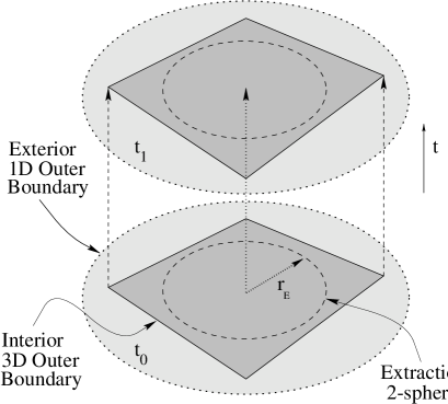
FIG. 1.: Location of the different outer boundaries and of the extraction 2-sphere for two successive timeslices. The dark shaded region shows the spatial domain over which the 3D nonlinear equation are solved.

The first step involves interpolating $K_{ij}$ and $\partial_{t}K_{ij}$ onto the 2-sphere and evaluating their projections onto the appropriate conjugate tensor spherical harmonics to eliminate the angular dependence and obtain the corresponding multipoles. The precise location of the 2-sphere within the interior 3D grid depends on the specific case under investigation. In general, for the perturbative matching to be justified, we require that the extraction surface be located in a region where the gravitational field is close to Schwarzschild. One must be careful that the numerical errors introduced by the interior evolution do not dominate the exterior solution. (Further details will be presented elsewhere [18].)

The second step entails evolving equations (7)–(12). In the test presented here, we consider a flat background with $M=0$. The initial data for the 1D exterior grid is set consistently with the interior 3D initial data. During each time integration of the 1D exterior grid, the extracted multipoles are used as inner boundary values and standard Sommerfeld outgoing wave conditions are imposed at the outer boundary (e.g., at $r=30$). The top diagram of Fig. 2 shows the only relevant multipole for this test [19], extracted from the interior 3D grid at a 2-sphere of radius $r_{{}_{E}}=1$ [20]; the lower diagram shows its evolved waveform at a radius $r=8$. Different curves refer to different resolutions of the interior 3D grid and show the convergence to the analytic solution.

FIG. 2.: Convergence to the analytic solution of the extracted ($r=1$) and evolved ($r=8$) multipole $(a_{+})_{20}$. The amplitude is scaled by $r^{3}$ to compensate for the radial fall-off.

The third and final step consists of computing outer boundary values for the interior 3D grid, and this step can proceed in one of two ways. In the first method, the values of $K_{ij}$ reconstructed from the exterior 1D data are injected as Dirichlet data at all the boundary points of the interior 3D grid. (No restrictions are put on the shape of the 2-surface where the data are injected.) For a code using a hyperbolic formulation, $\partial_{t}K_{ij}$ can also be provided at the boundary. Moreover, the evolution equation of the three-metric can be integrated using $K_{ij}$ at the boundary so Dirichlet data for $g_{ij}$ need not be provided there. The second method relates, at the 3D outer boundary, the null derivatives of the extrinsic curvature obtained from the interior grid ($K_{ij}$) and from the perturbative module ($\kappa_{ij}$, since background extrinsic curvature is assumed to be zero):

$${\partial\over\partial t}\left(K_{ij}-\kappa_{ij}\right)+{\partial\over\partial r}\left(K_{ij}-\kappa_{ij}\right)+{2\over r}\left(K_{ij}-\kappa_{ij}\right)=0$$ (13)

This method resembles a Sommerfeld condition but is more general since it can be used in regions where the radiation is not dominated by the asymptotic outgoing behavior. Moreover it takes into account arbitrary angular dependence, as well as the effects of a Schwarzschild black hole background. Experimentation with the two methods has shown that this “perturbative Sommerfeld” approach is very accurate and generally more stable than the direct injection of Dirichlet data. Figure 3 shows convergence to zero of the $L_{2}$ norm of the difference between one component of $K_{ij}$ (namely $K_{zz}$) and its analytic value, integrated over the entire outer boundary of the interior 3D grid.

FIG. 3.: Convergence to zero of the $L_{2}$ norm of the error of $K_{zz}$ integrated over the 3D outer boundary surface.

An important property of any outer boundary implementation is that it should allow the outgoing radiation to escape freely to infinity. In practice, however, a finite discretization always produces a certain amount of reflection at the outer boundary and this could drive instabilities which grow exponentially. We have compared the long-term stability obtained with the perturbative outer boundary module with that of the best “alternative” outer boundary conditions we have tried: namely a standard outgoing Sommerfeld condition. Fig. 4 shows the results of this comparison both on a long time scale and on a shorter time scale. (The calculations were performed using a very coarse resolution.) As shown in the inset (first echoes at $t\sim 7$), the amount of reflection produced with the perturbative method is smaller than that produced by the Sommerfeld condition. Moreover, the use of perturbative boundary conditions delays the onset of exponential error growth and allows for a much longer evolution (see main figure). Increasing the interior resolution and the number of $(\ell,m)$ modes used we can further prolong the running time. Using $(49)^{3}$ interior gridpoints, we are able to evolve the code for more than $50$ crossing times. In strong contrast, when a standard Sommerfeld condition is used, increased interior resolution results in a shorter running time [18].

FIG. 4.: Long-term evolution of the $L_{2}$ norm of the error in $K_{zz}$ at the 3D outer boundary surface. The inset shows $K_{zz}$ at the outer boundary along the $x-$axis. The interior grid has $(33)^{3}$ gridpoints and the code is stopped when the norm is unity.

This work was supported by the NSF Binary Black Hole Grand Challenge Grant Nos. NSF PHY 93–18152, NSF PHY 93–10083, ASC 93–18152 (ARPA supplemented). Computations were performed at NPAC (Syracuse University) and at NCSA (University of Illinois at Urbana-Champaign).

REFERENCES

- [1] Information about the Binary Black Hole Grand Chal-lenge Alliance, its goals and present status of research can be found at the web page: http://www.npac.syr.edu/projects/bh/.
- [2] R. Arnowitt, S. Deser and C. W. Misner, in Gravitation, edited by L. Witten, Wiley, New York (1962).
- [3] J. W. York in Sources of Gravitational Radiation, edited by L. Smarr, Cambridge Univ. Press, Cambridge (1979).
- [4] Y. Choquet-Bruhat and J. W. York in General Relativity and Gravitation I, edited by A. Held, Plenum, New York (1980).
- [5] E. Seidel and W.-M. Suen, Phys. Rev. Lett., 69, 1845 (1992).
- [6] A. M. Abrahams and C. R. Evans, Phys. Rev. D, 37, 317 (1988); Phys. Rev. D, 42, 2585 (1990).
- [7] A. M. Abrahams et al., Phys. Rev. D 45, 3544 (1992); P. Anninos et al., Phys. Rev. Lett. 71, 2851 (1993).
- [8] A. M. Abrahams, S. L. Shapiro and S. A. Teukolsky, Phys. Rev. D 51, 4295 (1995); A. M. Abrahams and R. H. Price, Phys. Rev. D 53, 1963, Ibidem, 1972 (1996).
- [9] N. T. Bishop, R. Gomez, P. R. Holvorcem, R. A. Matzner, P. Papadopoulos and J. Winicour Phys. Rev. Lett. 76, 4303 (1996); N. T. Bishop, R. Gomez, L. Lehner, J. Winicour Phys. Rev. D. 54, 6153 (1996).
- [10] T. Regge and J.A. Wheeler, Phys. Rev. 108, 1063 (1957); F. Zerilli, Phys. Rev. Lett. 24 737 (1970).
- [11] V. Moncrief, Annals of Physics 88, 323 (1974).
- [12] R. H. Price and J. Pullin, Phys. Rev. Lett. 72, 3297 (1994).
- [13] A. M. Abrahams and G. Cook, Phys. Rev. D , (1994).
- [14] Y. Choquet-Bruhat and J. W. York, C. R. Acad. Sci. Paris, 321, 1089 (1995); A. Abrahams, A. Anderson, Y. Choquet-Bruhat and J. W. York, Phys. Rev. Lett. 75, 3377 (1995).
- [15] A. M. Abrahams, A. Anderson, C. R. Evans, C. Lea, J. Lenaghan, M. Rupright and J. W. York, In preparation.
- [16] The Binary Black Hole Grand Challenge Alliance, In preparation.
- [17] S. Teukolsky, Phys. Rev. D 26, 745 (1982).
- [18] A. M. Abrahams, L. Rezzolla and M. Rupright, In preparation.
- [19] Other multipoles are also computed and used in the decomposition; but, given the initial data chosen, their amplitudes are several orders of magnitude smaller [18].
- [20] On a flat background spacetime, the position of the extraction 2-sphere is arbitrary. Similar results have been obtained also for [18].