Non-Abelian Black Holes in Brans-Dicke Theory

Abstract

We find a black hole solution with non-Abelian field in Brans-Dicke theory. It is an extension of non-Abelian black hole in general relativity. We discuss two non-Abelian fields: “SU(2)” Yang-Mills field with a mass (Proca field) and the SU(2)$\times$SU(2) Skyrme field. In both cases, as in general relativity, there are two branches of solutions, i.e., two black hole solutions with the same horizon radius. Masses of both black holes are always smaller than those in general relativity. A cusp structure in the mass-horizon radius ($M_{g}$-$r_{h}$) diagram, which is a typical symptom of stability change in catastrophe theory, does not appear in the Brans-Dicke frame but is found in the Einstein conformal frame. This suggests that catastrophe theory may be simply applied for a stability analysis as it is if we use the variables in the Einstein frame. We also discuss the effects of the Brans-Dicke scalar field on black hole structure.

I Introduction

For many years, there have been various efforts to find a theory of “everything”. The Kaluza-Klein theory was one of the candidates, which is constructed in a five dimensional spacetime. Jordan noticed in 1955 that in our four dimensional spacetime, a scalar field appears by a compactification in the Kaluza-Klein theory and it gives a nonminimal coupling to gravity, meaning that this theory violates even the weak equivalence principle. Dicke thought that the weak equivalence principle must be guaranteed based on several experiments. Then, from the weak equivalence principle and Mach’s Principle, which insists that an inertial force is determined by the distribution of matter all over the Universe, he and Brans constructed a new scalar-tensor theory, i.e., Brans-Dicke (BD) theory, in 1961[2]. Since then the difference between general relativity (GR) and BD theory has been discussed in many aspects. Although BD theory itself is strongly constrained by several experiments (the BD parameter $\omega\geq 500$), we believe that the theory may still be important from the following points of view:

1. BD theory can be an effective field theory of a unified theory of fundamental forces. In particular the BD-type scalar field appears as a dilaton field in superstring theory.

2. BD theory is one of the simplest extensions of GR. So if we wish to discuss something in a generalized theory of gravity, BD theory can be the best model to see a difference from GR.

Moreover, a scalar field such as the BD scalar field may have an affect on many aspects in gravitational physics. For example, the inflationary scenario would be modified by an introduction of such a scalar field[3]. Although the inflationary scenario was discussed originally in GR, since an appropriate model based on particle physics has not been found, it is important to recognize that the introduction of a scalar field can make a big change in scenarios of the very early universe.

Black holes are also important in gravitational physics. We may expect that such a scalar field also affects some feathers of a black hole[4]. However, since the gravity part in BD theory is conformally equivalent to that in GR, black hole solutions are not modified by the introduction of the BD scalar field for the case without matter or with a traceless matter field such as the electromagnetic field. As a result, for vacuum case or the case with the electromagnetic field, a conventional Kerr or Kerr-Newman black hole turns out to be a unique solution even in BD theory because of the black hole no-hair theorem in GR[5]. Hence, here we shall discuss a non-Abelian black hole in BD theory, which has so far not been studied so much. For the case with the Yang-Mills field, however, we again find the same colored black hole as that in GR[6], because its energy-momentum tensor is traceless. Then, we discuss a “massive” non-Abelian field, i.e., a massive Yang-Mills (Proca) field, and the Skyrme field. We consider only the globally neutral case in this paper.

After the introduction of basic ansätze and conditions in §.II, we present the Proca black hole solution and its properties in §.III. We find some difficulty in adopting catastrophe theory to the stability analysis. To resolve such a difficulty, we introduce new variables defined in the Einstein conformal frame in §.IV. We find quite similar properties of black hole solutions to those in GR: in particular a cusp structure appears in the mass-horizon radius diagram. This allows simple application of catastrophe theory in the stability analysis as it is. The effects of the BD scalar field on black hole structure are investigated in §.V. In §.VI, we discuss a Skyrme black hole, showing that its properties are quite similar to those in the Proca black hole. The concluding remarks will follow in §.VII. Throughout this paper we use units of c=$\hbar$=1. Notations and definitions such as Christoffel symbols and curvatures follow Misner-Thorne-Wheeler [7].

II Non-Abelian black holes in Brans-Dicke theory

The action of BD theory is written as

$$S=\int d^{4}x\sqrt{-g}\left[\frac{1}{2\kappa^{2}}\left(\phi R-\frac{\omega}{\phi}\nabla_{\alpha}\phi\nabla^{\alpha}\phi\right)+L_{m}\right]\ ,$$ (1)

where $\kappa^{2}\equiv 8\pi G$ with $G$ being Newton’s gravitational constant. The BD parameter is $\omega$, and $L_{m}$ is the Lagrangian of the matter field. The dimensionless BD scalar field $\phi$ is normalized by $G$.

For the BD field $\phi$, the field equation becomes

$$\Box\phi=\frac{\kappa^{2}}{2\omega+3}T^{\mu}_{\mu}\ .$$ (2)

Then, if the right hand side of this equation vanishes, that is, the energy-momentum tensor of the matter field is traceless, $\phi$= constant turns out to be a solution, meaning that a black hole solution in GR is also a solution in BD theory. Hence, for the SU(2) Yang-Mills field, we find that the colored black hole[6] is a solution in BD theory too. Although we have no proof, we expect that for the case with a massless non-Abelian gauge field, no new type of black hole solution appears in BD theory.

If a non-Abelian field is massive or effectively massive, however, $\phi$ = constant is no longer a solution. We will find a new type of black hole solution, and can discuss some differences from black hole solutions in GR. This is the reason for us to study a massive non-Abelian field here.

We assume that a black hole is static and spherically symmetric, in which case the metric is written as

$$ds^{2}=-\left[1-\frac{2Gm(r)}{r}\right]e^{-2\delta(r)}dt^{2}+\left[1-\frac{2Gm(r)}{r}\right]^{-1}dr^{2}+r^{2}d\Omega^{2}\ .$$ (3)

The boundary condition for a black hole solution at spatial infinity is

$$\lim_{r\rightarrow\infty}m=M<\infty,\ \lim_{r\rightarrow\infty}\delta=0,\ \lim_{r\rightarrow\infty}\phi=\phi_{0}\equiv\frac{2(2+\omega)}{3+2\omega}\ .$$ (4)

Note that a test particle far from a black hole does not move under an influence of this “mass” $M$, but feels a gravitational attractive force given by a gravitational mass $M_{g}$. $M_{g}$ is defined from the asymptotic behavior of the time-time component of the metric and given as

$$M_{g}=M+{1\over G}\lim_{r\rightarrow\infty}(r\delta)\ .$$ (5)

For the existence of a regular event horizon, $r_{h}$, we have

$$m_{h}\equiv m(r_{h})=\frac{r_{h}}{2G},\ \delta_{h}\equiv\delta(r_{h})<\infty\ .$$ (6)

We also require that no singularity exists outside the horizon, i.e.,

$$m(r)<\frac{r}{2G}\ ~{}~{}~{}~{}~{}{\rm for}~{}~{}~{}r>r_{h}.$$ (7)

For our numerical calculation, we introduce the following dimensionless variables:

$$\bar{r}=r/r_{h},\ \bar{m}=Gm/r_{h}.$$ (8)

To write down the explicit equations of motion, we have to specify our models. In what follows, we discuss the Proca field and the Skyrme field, separately.

III Proca Black Hole

We first consider a massive “SU(2)” Yang-Mills field (Proca field). The matter Lagrangian $L_{m}$ is now

$$L_{m}=-\frac{1}{16\pi g_{c}^{2}}{\rm Tr}\mbox{\boldmath$F$}^{2}-\frac{\mu^{2}}{8\pi g_{c}^{2}}{\rm Tr}\mbox{\boldmath$A$}^{2}\ ,$$ (9)

where $g_{c}$ and $\mu$ are the gauge coupling constant and the mass of the Proca field, respectively. $F$ is the field strength expressed by its potential $A$ as $\mbox{\boldmath$F$}=d\mbox{\boldmath$A$}+\mbox{\boldmath$A$}\wedge\mbox{\boldmath$A$}$. For the spherically symmetric case, we can write the vector potential as

$$\mbox{\boldmath$A$}=a(r,t)\mbox{\boldmath$\tau$}_{r}dt+\frac{b(r,t)}{r}\mbox{\boldmath$\tau$}_{r}dr+\{d(r,t)\mbox{\boldmath$\tau$}_{\theta}-[1+w(r,t)]\mbox{\boldmath$\tau$}_{\phi}\}d\theta$$ (10)

$$+\{[1+w(r,t)]\mbox{\boldmath$\tau$}_{\theta}+d(r,t)\mbox{\boldmath$\tau$}_{\phi}\}\sin\theta d\phi$$ (11)

as Witten showed[8], where $\mbox{\boldmath$\tau$}_{r},\mbox{\boldmath$\tau$}_{\theta}$, and $\mbox{\boldmath$\tau$}_{\phi}$ are the generators of su(2) Lie algebra. We adopt the ’t Hooft ansatz, i.e., $a\equiv 0$, which means that only a magnetic component of the Proca field exists. We also set $b=0$. In the static case, we can set $d=0$. Now, our potential is

$$\mbox{\boldmath$A$}=[1+w(r)](-\mbox{\boldmath$\tau$}_{\phi}d\theta+\mbox{\boldmath$\tau$}_{\theta}\sin\theta d\phi)\ .$$ (12)

The boundary condition of the Proca field for its total energy to be finite is

$$\lim_{r\rightarrow\infty}w=-1\ .$$ (13)

We define dimensionless parameters as

$$\bar{\mu}=\mu/(g_{c}m_{p}),\ \ \lambda_{h}=r_{h}/(l_{p}/g_{c})\ .$$ (14)

$l_{p}\equiv G^{1/2}$ and $m_{p}\equiv G^{-1/2}$ are the Planck length and mass defined by Newton’s gravitational constant, respectively.

Under the above ansätze, we find the following basic equations:

$$\frac{d\bar{m}}{d\bar{r}} = \left(2\phi+\bar{r}\frac{d\phi}{d\bar{r}}\right)^{-1}\left[\left(1-\frac{2\bar{m}}{\bar{r}}\right)\left\{\frac{\omega+2}{2\phi}\left(\bar{r}\frac{d\phi}{d\bar{r}}\right)^{2}+\frac{2}{\lambda_{h}^{2}}\left(\frac{dw}{d\bar{r}}\right)^{2}\right\}-\bar{m}\frac{d\phi}{d\bar{r}}\right.$$ (16)

$$+\left.\frac{1}{\lambda_{h}^{2}}\left(\frac{1-w^{2}}{\bar{r}}\right)^{2}\left(1+\frac{\bar{r}}{\phi}\frac{d\phi}{d\bar{r}}\right)+2(1+w)^{2}\bar{\mu}^{2}\left\{\frac{2\omega+1}{2\omega+3}+\frac{2(\omega+1)\bar{r}}{(2\omega+3)\phi}\frac{d\phi}{d\bar{r}}\right\}\right]\ ,$$

$$\frac{d\delta}{d\bar{r}} = -\frac{\bar{r}}{\phi}\left(2\phi+\bar{r}\frac{d\phi}{d\bar{r}}\right)^{-1}\left\{(\omega+1)\left(\frac{d\phi}{d\bar{r}}\right)^{2}+\frac{4}{\lambda_{h}^{2}}\frac{\phi}{\bar{r}^{2}}\left(\frac{dw}{d\bar{r}}\right)^{2}\right\}$$ (19)

$$-\bar{r}\left(2\phi+\bar{r}\frac{d\phi}{d\bar{r}}\right)^{-1}\left(1-\frac{2\bar{m}}{\bar{r}}\right)^{-1}\left[\frac{1}{\lambda_{h}^{2}}\frac{\bar{r}}{\phi}\frac{d\phi}{d\bar{r}}\left\{\left(\frac{1-w^{2}}{\bar{r}^{2}}\right)^{2}+\frac{4(\omega+1)\bar{\mu}^{2}\lambda_{h}^{2}}{2\omega+3}\left(\frac{1+w}{\bar{r}}\right)^{2}\right\}\right.$$

$$-\left.\frac{2}{\bar{r}}\left(1-\frac{\bar{m}}{\bar{r}}\right)\frac{d\phi}{d\bar{r}}-\frac{4\bar{\mu}^{2}}{2\omega+3}\left(\frac{1+w}{\bar{r}}\right)^{2}\right]\ ,$$

$$\frac{d^{2}\phi}{d\bar{r}^{2}} = \frac{1}{\phi}\left(\frac{d\phi}{d\bar{r}}\right)^{2}+\left(1-\frac{2\bar{m}}{\bar{r}}\right)^{-1}\left[\frac{1}{\lambda_{h}^{2}}\frac{\bar{r}}{\phi}\frac{d\phi}{d\bar{r}}\left\{\left(\frac{1-w^{2}}{\bar{r}^{2}}\right)^{2}+\frac{4(\omega+1)\bar{\mu}^{2}\lambda_{h}^{2}}{2\omega+3}\left(\frac{1+w}{\bar{r}}\right)^{2}\right\}\right.$$ (21)

$$-\left.\frac{2}{\bar{r}}\left(1-\frac{\bar{m}}{\bar{r}}\right)\frac{d\phi}{d\bar{r}}-\frac{4\bar{\mu}^{2}}{2\omega+3}\left(\frac{1+w}{\bar{r}}\right)^{2}\right]\ ,$$

$$\frac{d^{2}w}{d\bar{r}^{2}} = \frac{1}{\phi}\frac{dw}{d\bar{r}}\frac{d\phi}{d\bar{r}}+\left(1-\frac{2\bar{m}}{\bar{r}}\right)^{-1}\left[(1+w)\left\{\bar{\mu}^{2}\lambda_{h}^{2}-\frac{w(1-w)}{\bar{r}^{2}}\right\}-\frac{2\bar{m}}{\bar{r}^{2}}\frac{dw}{d\bar{r}}\right.$$ (23)

$$+\left.\frac{1}{\lambda_{h}^{2}}\frac{\bar{r}}{\phi}\frac{dw}{d\bar{r}}\left\{\left(\frac{1-w^{2}}{\bar{r}^{2}}\right)^{2}+\frac{4(\omega+1)\bar{\mu}^{2}\lambda_{h}^{2}}{(2\omega+3)}\left(\frac{1+w}{\bar{r}}\right)^{2}\right\}\right]\ .$$

As for the boundary condition at the event horizon, in order for the horizon to be regular, the square brackets in (19), (21) and (23) must vanish at the horizon $\bar{r}=1$. Hence, we find that

$$\frac{dw}{d\bar{r}}\bigg{|}_{\bar{r}=1} = -\frac{\phi_{h}\lambda_{h}^{2}(2\omega+3)(1+w_{h})\{\bar{\mu}^{2}\lambda_{h}^{2}-w_{h}(1-w_{h})\}}{(2\omega+3)\{(1-w^{2}_{h})^{2}-\phi_{h}\lambda_{h}^{2}\}+4\bar{\mu}^{2}(\omega+1)\lambda_{h}^{2}(1+w_{h})^{2}}\ ,$$ (24)

$$\frac{d\phi}{d\bar{r}}\bigg{|}_{\bar{r}=1} = \frac{4\bar{\mu}^{2}(1+w_{h})^{2}\lambda_{h}^{2}\phi_{h}}{(2\omega+3)\{(1-w^{2}_{h})^{2}-\phi_{h}\lambda_{h}^{2}\}+4\bar{\mu}^{2}(\omega+1)\lambda_{h}^{2}(1+w_{h})^{2}}\ ,$$ (25)

where $w_{h}\equiv w(r_{h})$ and $\phi_{h}\equiv\phi(r_{h})$. As a result, $w_{h}$ and $\phi_{h}$ turn out to be shooting parameters and should be determined iteratively so that the boundary conditions (4) and (13) are satisfied.

In Fig.1, we present a numerical solution with $r_{h}=0.5l_{p}/g_{c}$ and $\mu=0.15g_{c}m_{p}$. We set $\omega=0$. Although this is not consistent with the present limit from experiments, we choose this value because we wish to clarify the difference from black holes in GR. For a massive non-Abelian field, the node number of the potential $w(r)$ is limited by some finite integer. Here the node number is chosen to be the smallest value, i.e., one. The dotted line denotes the Proca black hole in GR[9] with the same parameters, i.e. $r_{h}=0.5l_{p}/g_{c}$ and $\mu=0.15g_{c}m_{p}$, which we show as a reference.

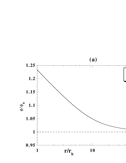
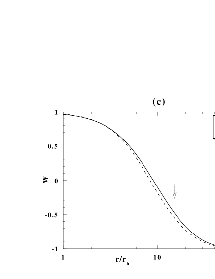
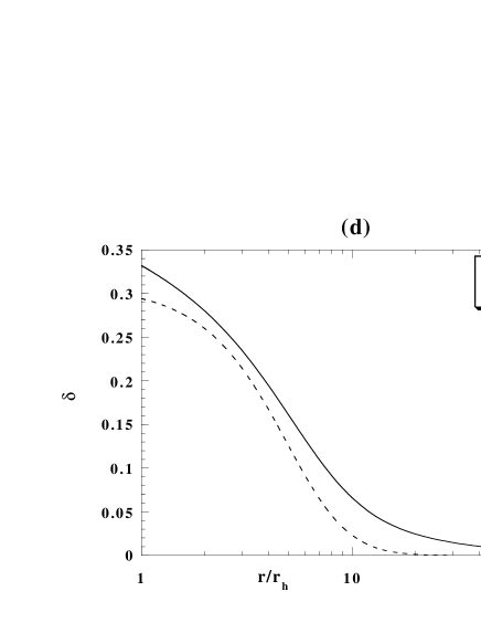
FIG. 1.: The solution of the Proca black hole in BD theory with $\omega=0$ for $r_{h}=0.5l_{p}/g_{c}$ and $\mu=0.15g_{c}m_{p}$( (a) $\phi(r)$, (b) $\bar{m}(r)$, (c) w(r), (d) $\delta$(r) ). : The Proca black hole in GR is also depicted as a reference by a dotted line. The arrow in (c) shows the Compton wavelength of the Proca field ($1/\mu$).

As seen from Fig.1(a), the BD scalar field decreases monotonically as

$$\phi \sim \phi_{0}\left(1+\frac{2GM_{s}}{r}\right)\ ,$$ (26)

where $M_{s}$ is a constant and called the scalar mass[10]. Fig.1(c) shows that the non-trivial structure of the non-Abelian field extends to the scale of the Compton wavelength of the Proca field ($\sim 1/\mu$), which is shown by an arrow. From Fig.1(d), you may not see a clear difference between the lapse function $\delta$ in BD theory and that in GR, but $\delta$ in BD theory falls as $1/r$ as $r\rightarrow\infty$ while $\delta$ in GR vanishes much faster than $1/r$. In fact, from Eq. (19) we find

$$\frac{d\delta}{dr}\sim\frac{1}{\phi}\frac{d\phi}{dr}\ \sim-\frac{2GM_{s}}{r^{2}}$$ (27)

near spatial infinity. This gives the relation between $M$ and $M_{g}$ as

$$M_{g}=M+2M_{s}\ .$$ (28)

To see a property of a family of black hole solutions, we show the relation between the gravitational mass $M_{g}$ and horizon radius $r_{h}$ in Fig.2. The dotted lines denote the Proca black hole in GR with the same parameters, i.e. $\mu=0.1g_{c}m_{p}$ or $\mu=0.15g_{c}m_{p}$, and the dot-dashed lines represent the Schwarzschild and colored black holes, respectively, which we show as references.

As we mentioned in Fig.1(c), the non-trivial structure of the non-Abelian field is as large as the scale of the Compton wavelength ($\sim 1/\mu$). This is responsible for the existence of a maximum horizon radius ($\sim 1/\mu$) as in GR. That is, beyond this critical horizon radius, a non-trivial structure is swallowed into the horizon and then cannot exist, resulting in a trivial Schwarzschild spacetime.

The Schwarzschild black hole is a trivial solution ($m=M_{g},\ \delta=0,\ \phi=\phi_{0}\$and$\ w=-1$), which has no upper bound for a mass or a horizon radius. If the YM field is massless, a family of colored black holes also exists as a non-trivial black hole, where the BD scalar field is $\phi=\phi_{0}=$ constant. There is also no upper bound for horizon radius as in GR.

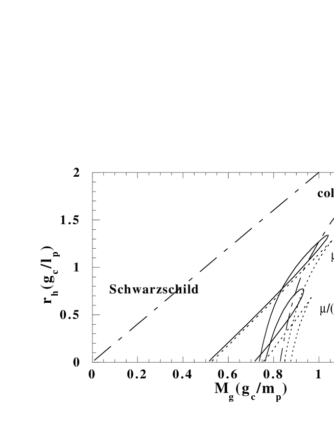
FIG. 2.: $M_{g}-r_{h}$ diagram of the Proca black holes. The solid loop lines denote Proca black holes with $\mu=0.1g_{c}m_{p}$ and $0.15g_{c}m_{p}$ in BD theory ($\omega=0$). We depict those in GR with the same parameters by dotted lines. The Schwarzschild and colored black holes are also shown as references.

The mass of the Proca black hole in BD theory is always smaller than that in GR (see also Fig.1(b)). This is just because the value of the BD scalar field near the black hole is larger than that at infinity, which means the effective gravitational constant is always smaller than $G$. Therefore the mass concentration by gravitational attractive force may get smaller.

In GR, there are two branches of black hole solutions: One is stable and the other is unstable. Those two branches coincide at a critical horizon radius or at a critical mass, where we find a cusp structure on the gravitational mass $M_{g}$- horizon radius $r_{h}$ diagram. This cusp structure is a typical symptom of stability change in catastrophe theory[11]. The stability analysis by catastrophe theory agrees with that by linear perturbations.

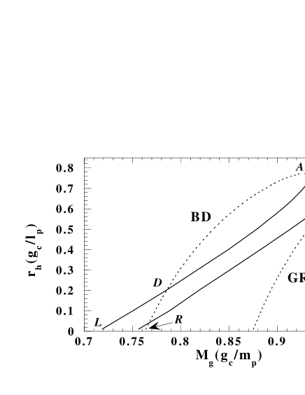
FIG. 3.: $M_{g}$-$r_{h}$ diagram for Proca black holes in BD theory ($\omega=0$) and in GR. The mass of the Proca field is $\mu=0.15g_{c}m_{p}$.

To see the detail and compare our solution with that in GR, we depict the enlarged diagram for $\mu=0.15g_{c}m_{p}$ in Fig.3. No cusp structure appears in BD theory. Though the solution curves seems to merge at the point D, we find two solutions exist at D, which can be distinguished from field distributions. In GR, the maximum points of horizon radius $r_{h}$ and of gravitational mass $M_{g}$ are the same, i.e., the point $C$ in Fig.3. In BD theory, however those two points, $A$ (maximum horizon radius) and $B$ (maximum gravitational mass), are different. This result does not depend on the choice of the BD parameter $\omega$ and the mass of the Proca field $\mu$. In particular, a cusp structure disappears in BD theory as mentioned above. One may wonder whether catastrophe theory can be simply applied to stability analysis as it is in BD theory, although it works quite well in GR[12]. For fixing $r_{h}$, we still have two solutions in BD theory as in GR. Is there any correspondence of those two solutions to two branches in GR? We expect that there are two types of black holes in the BD theory as well.

As we discussed in our previous papers[12], if we divide the total energy density $\rho_{total}$ into a kinetic term $\rho_{F^{2}}$ and a mass term $\rho_{A^{2}}$, one of the main differences between the two branches in GR (the solid-line and the dotted-line branches in Fig.3) comes from the difference of dominant ingredient, i.e., in the solid-line branch, $\rho_{A^{2}}$ is dominant compared to $\rho_{F^{2}}$, stabilizing a black hole solution. In the dotted-line branch, the situation is opposite. The stable solid-line branch is Schwarzschild type, while the unstable dotted-line branch is colored black hole type, in which the non-Abelian field and gravity balance each other.

In BD theory, if we divide the total energy density $\rho_{total}$ as

$$\rho_{total} = -T^{0}_{\ 0}=\rho_{A^{2}}+\rho_{F^{2}}+\rho_{\phi}\ ,$$ (29)

where

$$\rho_{A^{2}}\ (\frac{r_{h}}{m_{p}})^{2} = \frac{2(1+w)^{2}\bar{\mu}^{2}}{\bar{r}^{2}}\left(2\phi+\bar{r}\frac{d\phi}{d\bar{r}}\right)^{-1}\left\{\frac{2\omega+1}{2\omega+3}+\frac{2(\omega+1)\bar{r}}{(2\omega+3)\phi}\frac{d\phi}{d\bar{r}}\right\}\ ,$$ (30)

$$\rho_{F^{2}}\ (\frac{r_{h}}{m_{p}})^{2} = \frac{1}{\bar{r}^{2}\lambda_{h}^{2}}\left(2\phi+\bar{r}\frac{d\phi}{d\bar{r}}\right)^{-1}\left\{2\left(1-\frac{2\bar{m}}{\bar{r}}\right)\left(\frac{dw}{d\bar{r}}\right)^{2}+\left(\frac{1-w^{2}}{\bar{r}}\right)^{2}\left(1+\frac{\bar{r}}{\phi}\frac{d\phi}{d\bar{r}}\right)\right\}\ ,$$ (31)

$$\rho_{\phi}\ (\frac{r_{h}}{m_{p}})^{2} = \frac{1}{\bar{r}^{2}}\left(2\phi+\bar{r}\frac{d\phi}{d\bar{r}}\right)^{-1}\left\{\frac{\omega+2}{2\phi}\left(1-\frac{2\bar{m}}{\bar{r}}\right)\left(\bar{r}\frac{d\phi}{d\bar{r}}\right)^{2}-\bar{m}\frac{d\phi}{d\bar{r}}\right\}\ .$$ (32)

We find the similar behavior to the case in GR, i.e., $\rho_{A^{2}}$ is dominant to $\rho_{F^{2}}$ in the solid-line branch, while the opposite is true in the dotted-line branch (see Fig.4).

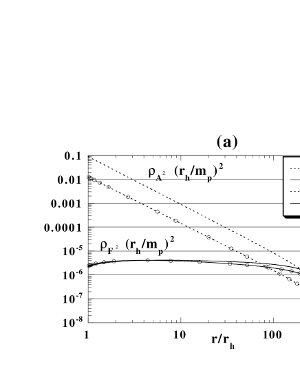
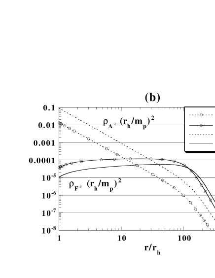
FIG. 4.: Distributions of the energy density for (a) the solid-line and (b) the dotted-line branches of the Proca black holes with $\mu=0.15g_{c}m_{p}$ both in BD theory ($\omega=0$) and in GR. The horizon radii of the black holes are $r_{h}=0.01l_{p}/g_{c}$.

In the solid-line branch, the black hole and non-Abelian structure are rather independent. In fact, a particle-like solution in this branch can exist without gravity. On the other hand, in the dotted-line branch, we need both the non-Abelian field and gravity. Then, we can divide the family of solutions into two: a sold-line branch from $A$ to $L$ (solid line) and a dotted-line branch from $R$ to $A$ (dotted line), respectively (see Fig.3). In the solid-line branch, the existence of the BD scalar field may not change the black hole structure, but it may affect a lot in the dotted-line branch. This is because the non-Abelian field in the solid-line branch does not give a dominant contribution to the black hole structure. As we will see later, this becomes more clear in the Einstein conformal frame, in which the effect of the BD scalar field is reduced to matter coupling.

For these two branches, we depict the scalar mass in terms of the horizon radius in Fig.5. The scalar mass $M_{s}$ in the solid-line branch is always larger than that in dotted-line branch. We also show the inverse temperature $1/T$ in terms of $M_{g}$ and the field strength at the horizon $B_{h}$ in terms of $r_{h}$ of Proca black holes with $\mu=0.15g_{c}m_{p}$ in Figs.7,7, which are quite similar to those in GR. $T$ and $B_{h}$ are defined by

$$T = \frac{1}{4\pi r}e^{-\delta}(1-2G\frac{dm}{dr})\bigg{|}_{\bar{r}=1}$$ (33)

$$B_{h} = ({\rm Tr}\mbox{\boldmath$F$}^{2})^{1/2}\bigg{|}_{\bar{r}=1}=\frac{\sqrt{2}(1-w_{h}^{2})}{r_{h}^{2}}\ .$$ (34)

Those also suggest that a stability may change somewhere in between $A$ (maximum horizon radius) and $B$ (maximum gravitational mass).

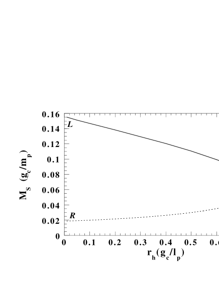
FIG. 5.: $r_{h}$-$M_{s}$ (scalar mass) diagram of the Proca black holes with $\mu=0.15g_{c}m_{p}$ in BD theory ($\omega=0$). The dotted and solid lines correspond to those in Fig.3.

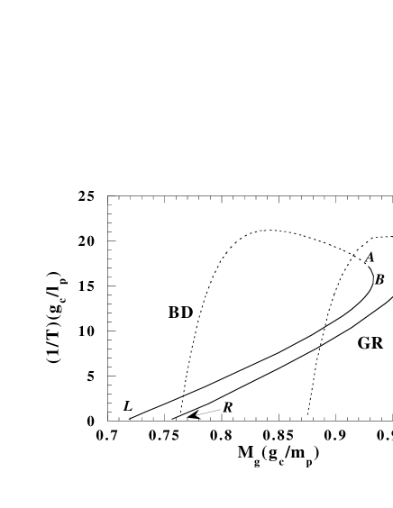
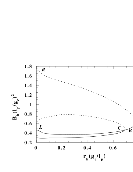
(a)       (b)

FIG. 6.: (a) $M_{g}$-$1/T$ diagram for Proca black holes with $\mu=0.15g_{c}m_{p}$ in BD theory ($\omega=0$) and in GR.

FIG. 7.: (b) $r_{h}$-$B_{h}$ diagram for Proca black holes with $\mu=0.15g_{c}m_{p}$ in BD theory ($\omega=0$) and in GR.

IV Proca Black Hole in the Einstein Conformal Frame

The gravity part of BD theory is conformally equivalent to that of GR, and a description by use of the Einstein conformal frame sometimes gives us simpler basic equations and easier analysis because the coupling of the BD scalar to gravity is moved to a matter term and the gravity part is just described as in the Einstein frame, which is already familiar. Hence, here we shall reanalyze our present problem in the Einstein conformal frame. We consider a conformal transformation

$$\hat{g}_{ab}=\frac{\phi}{\phi_{0}}g_{ab}\ .$$ (35)

The equivalent action $\hat{S}\equiv S/\phi_{0}$ is given as

$$\hat{S} = \displaystyle\int d^{4}x\sqrt{-\hat{g}}\left[\frac{1}{2\kappa^{2}}\hat{R}-\frac{1}{2}\hat{\nabla}_{\alpha}\varphi\hat{\nabla}^{\alpha}\varphi-{1\over\phi_{0}}\left(\frac{1}{16\pi g_{c}^{2}}{\rm Tr}\mbox{\boldmath$F$}^{2}+\frac{\mu^{2}}{8\pi g_{c}^{2}}\exp(-\kappa\beta\varphi){\rm Tr}\mbox{\boldmath$A$}^{2}\right)\right]\ ,$$ (37)

$$\ \ \ \ \varphi\equiv\frac{1}{\kappa\beta}\ln\left({\phi\over\phi_{0}}\right)\ ,\ \ \ \ \ \ \ \ \beta\equiv\left(\frac{2\omega+3}{2}\right)^{-1/2}.$$

For a black hole solution, if we define spherically symmetric coordinates in the Einstein frame as

$$d\hat{s}^{2} \equiv \frac{\phi}{\phi_{0}}ds^{2}$$ (38)

$$= -\left[1-\frac{2G\hat{m}(\hat{r})}{\hat{r}}\right]e^{-2\hat{\delta}(\hat{r})}dt^{2}+\left[1-\frac{2G\hat{m}(\hat{r})}{\hat{r}}\right]^{-1}d\hat{r}^{2}+\hat{r}^{2}d\Omega^{2}\ ,$$ (39)

we find

$$\hat{M}\equiv\lim_{\hat{r}\rightarrow\infty}\hat{m}(\hat{r})=M_{g}-M_{s},\ \ \ \hat{r}_{h}=r_{h}\sqrt{\frac{\phi_{h}}{\phi_{0}}}\ ,$$ (40)

where variables with a caret $\hat{}$ denote those in the Einstein frame. We also introduce dimensionless variables and parameters as

$$\bar{\hat{r}}=\hat{r}/\hat{r}_{h}\ ,\ \bar{\hat{m}}=G\hat{m}/\hat{r}_{h}\ ,\ \hat{\lambda}_{h}=\hat{r}_{h}g_{c}/l_{p}\ ,\ \bar{\varphi}=\varphi/m_{p}\ .$$ (41)

The basic equations are now

$$\frac{d\bar{\hat{m}}}{d\bar{\hat{r}}} = \left\{\frac{1}{\phi_{0}\hat{\lambda}_{h}^{2}}\left(\frac{dw}{d\bar{\hat{r}}}\right)^{2}+2\pi\bar{\hat{r}}^{2}\left(\frac{d\bar{\varphi}}{d\bar{\hat{r}}}\right)^{2}\right\}\left(1-\frac{2\bar{\hat{m}}}{\bar{\hat{r}}}\right)+\frac{1}{2\phi_{0}\hat{\lambda}_{h}^{2}}\left(\frac{1-w^{2}}{\bar{\hat{r}}}\right)^{2}$$ (43)

$$+\frac{\bar{\mu}^{2}}{\phi_{0}}\exp{(-\sqrt{8\pi}\beta\bar{\varphi})}(1+w)^{2}\ ,$$

$$\frac{d\hat{\delta}}{d\bar{\hat{r}}} = -4\pi\bar{\hat{r}}\left(\frac{d\bar{\varphi}}{d\bar{\hat{r}}}\right)^{2}-\frac{2}{\phi_{0}\hat{\lambda}_{h}^{2}\bar{\hat{r}}}\left(\frac{dw}{d\bar{\hat{r}}}\right)^{2}\ ,$$ (44)

$$\frac{d^{2}\bar{\varphi}}{d\bar{\hat{r}}^{2}} = -\frac{2}{\bar{\hat{r}}}+\left(1-\frac{2\bar{\hat{m}}}{\bar{\hat{r}}}\right)^{-1}\left[\left(\frac{d\bar{\varphi}}{d\bar{\hat{r}}}\right)\left\{-\frac{2\bar{\hat{m}}}{\bar{\hat{r}}^{2}}+\frac{\bar{\hat{r}}}{\phi_{0}\hat{\lambda}_{h}^{2}}\left(\frac{1-w^{2}}{\bar{\hat{r}}^{2}}\right)^{2}+2\bar{\hat{r}}\frac{\bar{\mu}^{2}}{\phi_{0}}\exp{(-\sqrt{8\pi}\beta\bar{\varphi})}\left(\frac{1+w}{\bar{\hat{r}}}\right)^{2}\right\}\right.$$ (46)

$$\left.-\frac{\bar{\mu}^{2}\beta\sqrt{8\pi}}{4\pi\phi_{0}}\exp{(-\sqrt{8\pi}\beta\bar{\varphi})}\left(\frac{1+w}{\bar{\hat{r}}}\right)^{2}\right]\ ,$$

$$\frac{d^{2}w}{d\bar{\hat{r}}^{2}} = \left(1-\frac{2\bar{\hat{m}}}{\bar{\hat{r}}}\right)^{-1}\left[\frac{dw}{d\bar{\hat{r}}}\left\{-\frac{2\bar{\hat{m}}}{\bar{\hat{r}}^{2}}+\frac{\bar{\hat{r}}}{\phi_{0}\hat{\lambda}_{h}^{2}}\left(\frac{1-w^{2}}{\bar{\hat{r}}^{2}}\right)^{2}+2\bar{\hat{r}}\frac{\bar{\mu}^{2}}{\phi_{0}}\exp{(-\sqrt{8\pi}\beta\bar{\varphi})}\left(\frac{1+w}{\bar{\hat{r}}}\right)^{2}\right\}\right.$$ (48)

$$\left.-\frac{w(1-w^{2})}{\bar{\hat{r}}^{2}}+\bar{\mu}^{2}\hat{\lambda_{h}^{2}}\exp{(-\sqrt{8\pi}\beta\bar{\varphi})}(1+w)\right]\ .$$

As we expected, these are simpler than those described in the BD frame. The boundary conditions are similar to the ones in the BD frame. From our numerical calculation, we can show that $\hat{M}=\hat{M}_{g}$ because $\hat{\delta}$ vanishes faster than $\hat{r}^{-1}$.

First, in Fig.9, we show the $\hat{M}_{g}$-$\hat{r}_{h}$ diagram in the Einstein frame that is related to Fig.3 by conformal transformation. Surprisingly, we recover a cusp structure even in BD theory. The solid-line is always located above the dotted-line branch as in GR. We also show the inverse temperature $1/T$ in terms of the gravitational mass $\hat{M}_{g}$ in Fig.9. Both figures show that the properties of the Proca black holes in BD theory are quite similar to those in GR.

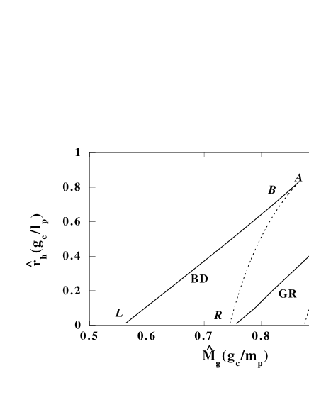
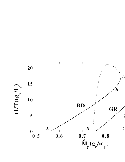
(a)       (b)

FIG. 8.: (a) $\hat{M}_{g}$-$\hat{r}_{h}$ diagram in the Einstein frame for Proca black holes in BD theory ($\omega=0$) and in GR. The mass of the Proca field is $\mu=0.15g_{c}m_{p}$. We find a cusp structure, which indicates a stability change via catastrophe theory.

FIG. 9.: (b) $\hat{M}_{g}$-$1/T$ diagram in the Einstein frame for Proca black holes in BD theory ($\omega=0$) and in GR. The mass of the Proca field is $\mu=0.15g_{c}m_{p}$.

This suggests that catastrophe theory will be simply applied in a stability analysis for non-Abelian black holes in BD theory as well.

From the point of view of catastrophe theory[11], stability changes at a cusp point in the control parameter-potential function diagram. In GR, if we regard gravitational mass and black hole entropy (or equivalently the area of the event horizon) as a control parameter and a potential function, respectively, we find a cusp $C$ in the $M_{g}$-$r_{h}$ ($\hat{M}_{g}$-$\hat{r}_{h}$) diagram (Figs.3,9), which is a symptom of stability change in catastrophe theory. In fact the stability of the black hole does change at this cusp point $C$. In BD theory, however, a cusp structure does not appear in Fig.3, while it does in Fig.9. This suggests that if we use the variables in the Einstein frame, we can simply apply catastrophe theory to the stability analysis in BD theory as it is. From Fig.9, catastrophe theory predicts that stability change can occur at the point $A$. From Fig.3, however, no such prediction is possible.

To study stability, we have another method, i.e., a turning point method for thermodynamical variables[13]. Stability will change at the point where $d(1/T)/dM=\infty$. In GR, we understand that a stability change occurs at the point $C$ in Figs.7,9. This is consistent with analysis by catastrophe theory. In BD theory, $d(1/T)/dM=\infty$ occurs at the point $B$ in Fig.7 (BD frame), which is inconsistent with the stability analysis by catastrophe theory. However, if we use the $\hat{M}_{g}$-$1/T$ diagram in the Einstein frame, the divergence occurs at the point $A$, which is consistent with catastrophe theory. To understand this inconsistency, we have to remember that variables in the turning point method should satisfy thermodynamical laws, in particular the “mass” of a black hole should satisfy the first law of black hole thermodynamics. In fact, the gravitational mass in the BD frame does not satisfy the first law of black hole thermodynamics, while it does so for the variables in the Einstein frame (Fig.9), and therefore the turning point method could be applied. We expect that a stability change occurs at the point $A$ but not at the point $B$, and this is consistent with catastrophe theory.

These conjectures for stability should be justified by analyzing linear perturbations of black holes and black hole thermodynamics[14].

V The Effects of the Brans-Dicke Scalar Field

By use of the Einstein frame, we also understand easily a qualitative difference between black holes in BD theory and in GR. As we see in the action (37), the coupling of the BD scalar field appears in the mass term. This coupling reduces effectively the mass of the Proca field by a factor $\exp(-\kappa\beta\varphi/2)$ because $\varphi$ is monotonically decreasing to zero as $r\rightarrow\infty$ (see Fig.1(a)). In GR, as the mass is reduced, the Proca black hole shifts in the left-upper direction in the $M_{g}$-$r_{h}$ diagram (see Fig.2). In fact, in the limit of zero mass, we recover Schwarzschild and colored black hole branches. As a result, for a fixed Proca field mass $\mu$, the black hole solution in BD theory also shifts in the left-upper direction from that in GR because of the coupling. Another contribution is $\phi_{0}$, which appears in the matter Lagrangian. Since $\phi_{0}^{-1}$ is its overall factor, this effect is renormalized by a redefinition of the gauge coupling constant $g_{c}$, i.e., $g_{c}^{\prime}=\sqrt{\phi_{0}}g_{c}$. As $\phi_{0}$ changes monotonically from 1 to $\infty$ for $\infty>\omega>-3/2$, the effective gauge coupling constant $g_{c}^{\prime}$ changes from $g_{c}$ to $\infty$.

The effects of the BD scalar field are divided into two:
(1) The gauge coupling constant is renormalized as $g_{c}^{\prime}=\sqrt{\phi_{0}}g_{c}$, which gives a stronger coupling than that in GR.
(2) The Brans-Dicke scalar field decreases as $r\rightarrow\infty$, which gives an effective change of the mass of the Proca field, i.e., $\mu^{\prime}=\mu\exp(-\kappa\beta\varphi/2)$.

In order to see the difference between BD theory and GR more clearly, we show the $\omega$ dependence of the black hole solutions in Figs.10,11, and 12.

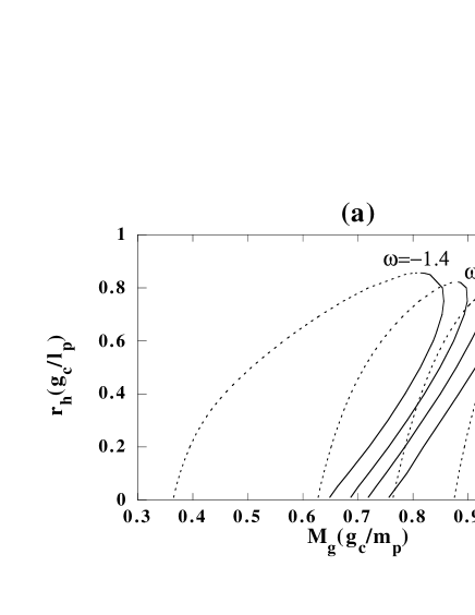
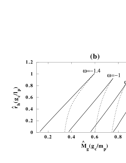
FIG. 10.: (a) $M_{g}$-$r_{h}$ diagram in the BD frame (b) $\hat{M}_{g}$-$\hat{r}_{h}$ diagram in the Einstein frame for several values of $\omega$. The mass of the Proca field is $\mu=0.15g_{c}m_{p}$.

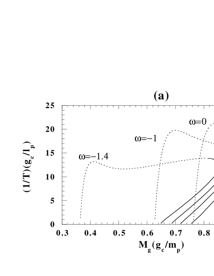
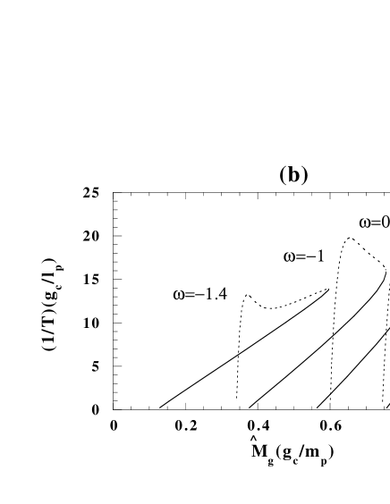
FIG. 11.: (a) $M_{g}$-$1/T$ diagram in the BD frame (b) $\hat{M}_{g}$-$1/T$ diagram in the Einstein frame for several values of $\omega$. The mass of the Proca field is $\mu=0.15g_{c}m_{p}$.

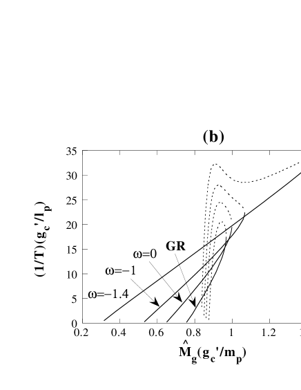
FIG. 12.: (a) $\hat{M}_{g}$-$r_{h}$ diagram and (b) $\hat{M}_{g}$-$1/T$ diagram normalized by $g_{c}^{\prime}=\sqrt{\phi_{0}}$ $g_{c}$ in the Einstein frame for several values of $\omega$. The mass of the Proca field is $\mu=0.15g_{c}m_{p}$.

From Fig.12, in which the effect is absorbed in normalization by $g_{c}^{\prime}$, we find the deviation from GR is quite similar to the behavior when changing a mass of the Proca field in GR (see Fig.2). This means that effects (1) and (2) really explain the deviation from GR.

In Fig.13, we depict the gravitational mass and the lapse function in terms of $\omega$ for fixed horizon radius ($r_{h}=0.5l_{p}/g_{c}$) and fixed mass of the Proca field ($\mu=0.15g_{c}m_{p}$). The solid and dotted lines correspond to those in the solid-line and in the dotted-line branches, respectively. Note that, when we fix the horizon radius in the BD frame (or in the Einstein frame), the horizon radius in the Einstein frame (or in the BD frame) will change for different values of $\omega$.

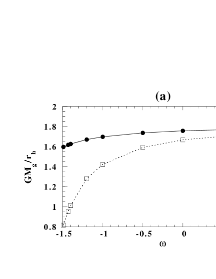
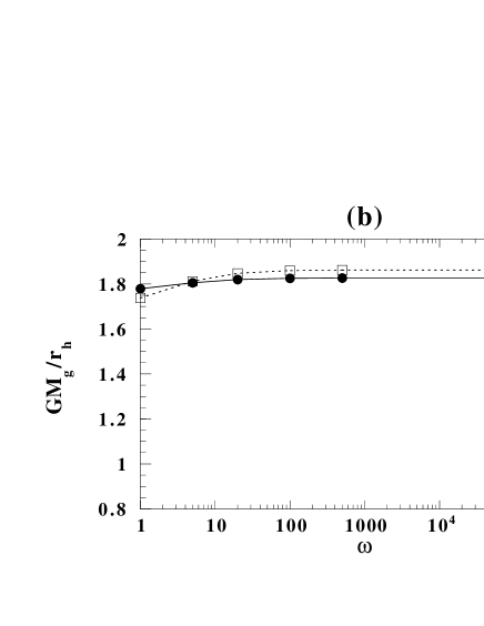
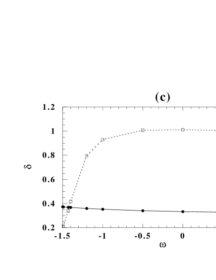
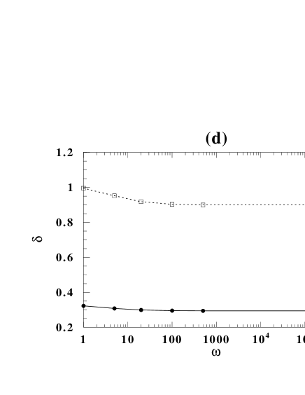
FIG. 13.: $\omega$ dependence on the gravitational mass $M_{g}$ and the lapse function $\delta$ of the Proca black hole in the BD frame for a fixed $r_{h}=0.5l_{p}/g_{c}$ and $\mu=0.15g_{c}m_{p}$ ((a) , (c) : $\omega\leq 1$ and (b) , (d) : $\omega\geq 1$). The dotted and solid lines correspond to the dotted- and solid-line branches in Fig.10.

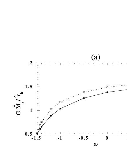
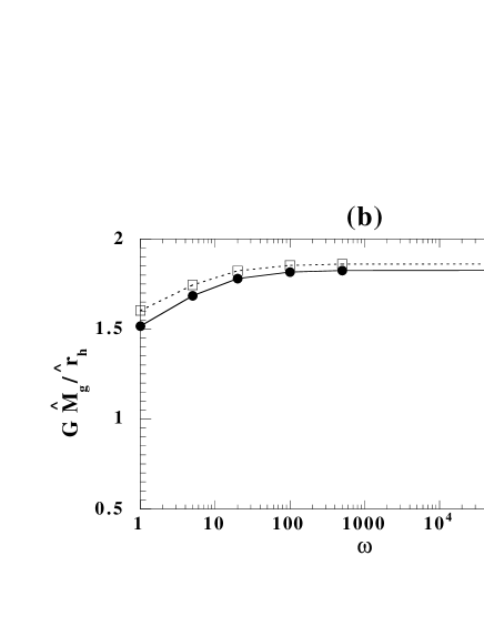
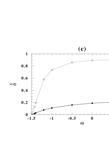
FIG. 14.: $\omega$ dependence on the gravitational mass $\hat{M}_{g}$ and the lapse function $\hat{\delta}$ of the Proca black hole in the Einstein frame for a fixed $r_{h}=0.5l_{p}/g_{c}$ and $\mu=0.15g_{c}m_{p}$ ((a) , (c) : $\omega\leq 1$ and (b) , (d) : $\omega\geq 1$). The dotted and solid lines correspond to the dotted- and solid-line branches in Fig.10.

We can see that the gravitational mass approaches some constants as $\omega\rightarrow\infty$, which correspond to those in GR. In the Einstein frame, the horizon radii in both branches approach the Schwarzschild radius in the limit of $\omega=-3/2$, resulting in a trivial Schwarzschild black hole(Fig.14).

This is because the matter contribution will vanish in this limit as we discussed above ($\phi_{0}^{-1}\rightarrow 0$). In the BD frame, however, we find that the dotted-line branch changes faster than the solid-line branch and both horizon radii in the limit of $\omega=-3/2$ are different from the Schwarzschild radius. Then non-trivial black holes can exist even for $\omega=-3/2$. This is consistent with the above result in the Einstein frame because the conformal transformation becomes singular for $\omega=-3/2$.

Although any value of $\omega>-3/2$ does not give a ghost, we find a negative mass contribution in the BD frame, resulting in that $M$ becomes negative for $\omega<(\omega_{cr}<-1)$. We show $m(r)$ for several values of $\omega$ in Fig.16. This does not mean, however, that we have a negative-mass black hole, because the gravitational mass $M_{g}$ is still positive. A test particle moving around a black hole feels an attractive force given by $M_{g}$, which is always positive. The effect of negative $M$ could be observed in a time delay, which changes its sign for negative $M$[10].

In the Einstein frame, $\hat{m}(r)$ is monotonically increasing as $r\rightarrow\infty$, resulting in a positive mass $\hat{M}$, which is the same as the gravitational mass $\hat{M}_{g}$ (Fig.16). As we know, in BD theory, we can define several masses[10]. The reason why we have several masses is because the BD scalar field decreases as $r^{-1}$, which is responsible for having different masses in each frame, and the scalar field itself also gives a contribution into a mass energy as a scalar mass $M_{s}$. In the vacuum case, we find a negative $M$ for $\omega<-1$. In our case, however, the BD scalar field is concentrated by the gravitational attractive force of the black hole. This changes the sensitivity $s$ just as for a self-gravitating star. From the asymptotic behavior of $g_{00}$ and $g_{rr}$, we find a relation between $M$ and $M_{g}$ as

$$\frac{M_{g}}{M}=\frac{\omega+2-s}{\omega+1+s}\ ,$$ (49)

where $s$ is a sensitivity (see Eq.(11.83) in [10]). Then the sensitivity $s$ could be evaluated as

$$s=\frac{1}{2}-\frac{(2\omega+3)(M_{g}-M)}{2(M+M_{g})}\ .$$ (50)

For a Schwarzschild black hole ($M=M_{g}$), $s=1/2$. If $\omega=-3/2$, however, $s=1/2$ even if $M\neq M_{g}$. We show the sensitivity $s$ in Fig.17. From Eq.(49), $M$ becomes negative for $\omega<-(1+s)\ (<-1)$. Then for a given $\omega\ (<-1)$, $M$ of the Proca black hole with smaller sensitivity than $s_{cr}\equiv-(1+\omega)$ becomes negative. It may correspond to smaller black holes in the solid-line branch from Fig.17. When $\omega\rightarrow\infty$, we find $M=M_{g}$ but $s\neq 1/2$. The reason is that the mass difference $M_{g}-M$(or $2M_{s}$) decreases as $\omega^{-1}$ for $\omega\rightarrow\infty$ (see Eq.(11.85) in [10]). While, as $\omega\rightarrow-3/2$, $s\rightarrow 1/2$ but $M_{g}\neq M$ (or $M_{s}\neq 0$) (see Fig.18). This is consistent with the previous fact that there still exists a nontrivial black hole in the limit of $\omega\rightarrow-3/2$.

(a)       (b)

FIG. 15.: (a) The mass function $m(r)$ with $r_{h}=0.5l_{p}/g_{c}$ and $\mu=0.15g_{c}m_{p}$ in the BD frame for several values of $\omega$.

FIG. 16.: (b) The mass function $\hat{m}(\hat{r})$ in the Einstein frame for several values of $\omega$. As in Fig. 16, we set $\mu=0.15g_{c}m_{p}$ and $r_{h}=0.5l_{p}/g_{c}$, which means that $\hat{\lambda}_{h}$ is not fixed in this figure.

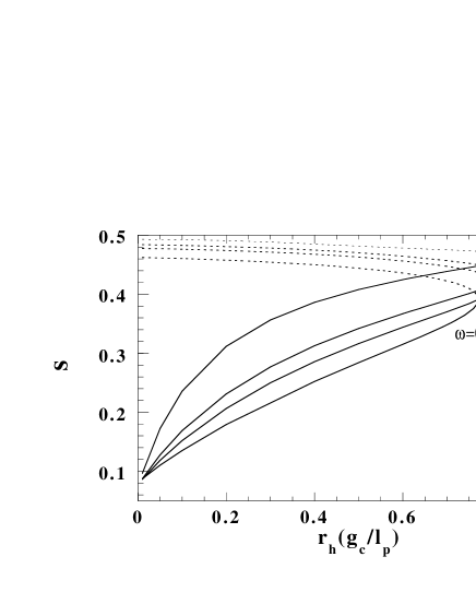
FIG. 17.: $r_{h}$-$s$ diagram for several values of $\omega$. The mass of the Proca field is $\mu=0.15g_{c}m_{p}$. The dotted and solid lines correspond to the dotted- and solid-line branches in Fig.10.

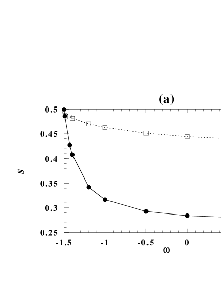
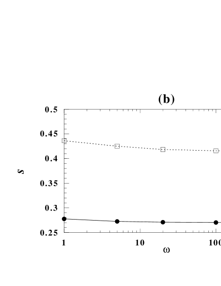
FIG. 18.: $\omega$ dependence on the sensitivity $s$ of the Proca black hole for a fixed $r_{h}=0.5l_{p}/g_{c}$ and $\mu=0.15g_{c}m_{p}$ ((a) $\omega\leq 1$ and (b) $\omega\geq 1$). The dotted and solid lines correspond to the dotted- and solid-line branches in Fig.10.

VI Skyrme Black Hole

In GR, non-trivial black holes with a massive non-Abelian field have quite similar properties, which we classified as Type II in [12]. How about black holes in BD theory? To see whether the above results for the Proca black hole are generic or not, we shall study the Skyrme field as another example of a “massive” non-Abelian field.

The action of the Skyrme field $L_{m}$ is $SU(2)\times SU(2)$ invariant and given as[15]

$$L_{m}=-\frac{1}{32g_{s}^{2}}{\rm Tr}\mbox{\boldmath$F$}^{2}-\frac{f_{s}^{2}}{4}{\rm Tr}\mbox{\boldmath$A$}^{2}\ ,$$ (51)

where $f_{s}$ and $g_{s}$ are coupling constants. $g_{s}$ is related to $g_{c}$ for the Proca field as

$$g_{s}=\sqrt{4\pi}g_{c}\ .$$ (52)

The “mass” parameter of the Skyrme field, $\mu$, is defined by $\mu=f_{s}g_{s}$. $F$ and $A$ are the field strength and its potential, respectively. They are described by the $SU(2)$-valued function $U$ as

$$\mbox{\boldmath$F$}=\mbox{\boldmath$A$}\wedge\mbox{\boldmath$A$},~{}~{}~{}\mbox{\boldmath$A$}=\mbox{\boldmath$U$}^{{\dagger}}\nabla\mbox{\boldmath$U$}\ .$$ (53)

In the spherically symmetric and static case, we can set $U$,

$$\mbox{\boldmath$U$}(\chi)=\cos\chi(r)+i\sin\chi(r)\mbox{\boldmath$\sigma$}_{i}\hat{r}^{i}\ ,$$ (54)

where $\mbox{\boldmath$\sigma$}_{i}$ and $\hat{r}^{i}$ are the Pauli spin matrices and a radial normal, respectively. The boundary condition for the total field energy to be finite is

$$\lim_{r\rightarrow\infty}\chi=0\ .$$ (55)

For simplicity, we solve the present system in the Einstein frame. The equivalent action $\hat{S}\equiv S/\phi_{0}$ is

$$\hat{S}=\displaystyle\int d^{4}x\sqrt{-\hat{g}}\left[\frac{\hat{R}}{2\kappa^{2}}-\frac{1}{2}\varphi_{,\alpha}\varphi^{,\alpha}-{1\over\phi_{0}}\left(\frac{1}{32g_{s}^{2}}{\rm Tr}\mbox{\boldmath$F$}^{2}+\frac{f_{s}^{2}}{4}\exp{(-\kappa\beta\varphi)}{\rm Tr}\mbox{\boldmath$A$}^{2}\right)\right]\ .$$ (56)

With the dimensionless parameter $\bar{f}_{s}\equiv f_{s}/m_{p}$, the basic equations are now

$$\frac{d\bar{\hat{m}}}{d\bar{\hat{r}}} = 2\pi\left[\bar{\hat{r}}^{2}\left(1-\frac{2\bar{\hat{m}}}{\bar{\hat{r}}}\right)\left\{\left(\frac{d\bar{\varphi}}{d\bar{\hat{r}}}\right)^{2}+\left(\frac{d\chi}{d\bar{\hat{r}}}\right)^{2}\left(\frac{\bar{f}_{s}^{2}}{\phi_{0}}\exp{(-\sqrt{8\pi}\beta\bar{\varphi})}+\frac{\sin^{2}\chi}{2\pi\phi_{0}\hat{\lambda}_{h}^{2}\bar{\hat{r}}^{2}}\right)\right\}\right.$$ (58)

$$\left.+\sin^{2}\chi\left(2\frac{\bar{f}_{s}^{2}}{\phi_{0}}\exp{(-\sqrt{8\pi}\beta\bar{\varphi})}+\frac{\sin^{2}\chi}{4\pi\phi_{0}\hat{\lambda}_{h}^{2}\bar{\hat{r}}^{2}}\right)\right]\ ,$$

$$\frac{d\hat{\delta}}{d\bar{\hat{r}}} = -4\pi\bar{\hat{r}}\left\{\left(\frac{d\bar{\varphi}}{d\bar{\hat{r}}}\right)^{2}+\left(\frac{d\chi}{d\bar{\hat{r}}}\right)^{2}\left(\frac{\bar{f}_{s}^{2}}{\phi_{0}}\exp{(-\sqrt{8\pi}\beta\bar{\varphi})}+\frac{\sin^{2}\chi}{2\pi\phi_{0}\hat{\lambda}_{h}^{2}\bar{\hat{r}}^{2}}\right)\right\}\ ,$$ (59)

$$\frac{d^{2}\bar{\varphi}}{d\bar{\hat{r}}^{2}} = \left(1-\frac{2\bar{\hat{m}}}{\bar{\hat{r}}}\right)^{-1}\left[\frac{d\bar{\varphi}}{d\bar{\hat{r}}}\left\{\frac{\sin^{2}\chi}{\bar{\hat{r}}}\left(8\pi\frac{\bar{f}_{s}^{2}}{\phi_{0}}\exp{(-\sqrt{8\pi}\beta\bar{\varphi})}+\frac{\sin^{2}\chi}{\phi_{0}\hat{\lambda}_{h}^{2}\bar{\hat{r}}^{2}}\right)-\frac{2\bar{\hat{m}}}{\bar{\hat{r}}^{2}}\right\}\right.$$ (62)

$$\left.-\sqrt{8\pi}\beta\frac{\bar{f}_{s}^{2}}{\phi_{0}}\exp{(-\sqrt{8\pi}\beta\bar{\varphi})}\frac{\sin^{2}\chi}{\bar{\hat{r}}^{2}}\right]$$

$$-\frac{2}{\bar{\hat{r}}}\frac{d\bar{\varphi}}{d\bar{\hat{r}}}-\frac{\sqrt{8\pi}\beta\bar{f}_{s}^{2}}{2\phi_{0}}\exp{(-\sqrt{8\pi}\beta\bar{\varphi}})\left(\frac{d\chi}{d\bar{\hat{r}}}\right)^{2}\ ,$$

$$\frac{d^{2}\chi}{d\bar{\hat{r}}^{2}} = -\frac{\exp{(-\sqrt{8\pi}\beta\bar{\varphi})}}{4\pi\bar{\hat{r}}^{2}\hat{\lambda}_{h}^{2}\bar{f}_{s}^{2}\exp{(-\sqrt{8\pi}\beta\bar{\varphi})}+2\sin^{2}\chi}\left(8\pi\hat{\lambda}_{h}^{2}\bar{f}_{s}^{2}\bar{\hat{r}}-4\pi\sqrt{8\pi}\beta\bar{\hat{r}}^{2}\hat{\lambda}_{h}^{2}\bar{f}_{s}^{2}\frac{d\bar{\varphi}}{d\bar{\hat{r}}}+\frac{d\chi}{d\bar{\hat{r}}}\sin 2\chi\right)\frac{d\chi}{d\bar{\hat{r}}}$$ (65)

$$+\left(1-\frac{2\bar{\hat{m}}}{\bar{\hat{r}}}\right)^{-1}\left[\frac{\sin 2\chi}{4\pi\bar{\hat{r}}^{2}\hat{\lambda}_{h}^{2}\bar{f}_{s}^{2}\exp{(-\sqrt{8\pi}\beta\bar{\varphi})}+2\sin^{2}\chi}\left(4\pi\hat{\lambda}_{h}^{2}\bar{f}_{s}^{2}\exp{(-\sqrt{8\pi}\beta\bar{\varphi})}+\frac{\sin^{2}\chi}{\bar{\hat{r}}^{2}}\right)\right.$$

$$+\left.\frac{d\chi}{d\bar{\hat{r}}}\left\{\frac{\sin^{2}\chi}{\bar{\hat{r}}}\left(8\pi\frac{\bar{f}_{s}^{2}}{\phi_{0}}\exp{(-\sqrt{8\pi}\beta\bar{\varphi})}+\frac{\sin^{2}\chi}{\phi_{0}\hat{\lambda}_{h}^{2}\bar{\hat{r}}^{2}}\right)-\frac{2\bar{\hat{m}}}{\bar{\hat{r}}^{2}}\right\}\right]\ .$$

As in the case of the Proca black hole, the square brackets in (62) and (65) must vanish at $r_{h}$ for the horizon to be regular. Hence

$$\frac{d\chi}{d\bar{r}}\bigg{|}_{\bar{r}=1} = -\frac{\phi_{0}\hat{\lambda}_{h}^{2}\sin 2\chi_{h}(4\pi\bar{f}_{s}^{2}\hat{\lambda}_{h}^{2}e^{-\sqrt{8\pi}\beta\bar{\varphi}_{h}}+\sin^{2}\chi_{h})}{(4\pi\bar{f}_{s}^{2}\hat{\lambda}_{h}^{2}e^{-\sqrt{8\pi}\beta\bar{\varphi}_{h}}+2\sin^{2}\chi_{h})\{\sin^{2}\chi_{h}(8\pi\bar{f}_{s}^{2}\hat{\lambda}_{h}^{2}e^{-\sqrt{8\pi}\beta\bar{\varphi}_{h}}+\sin^{2}\chi_{h})-\phi_{0}\hat{\lambda}_{h}^{2}\}}\ ,$$ (66)

$$\frac{d\bar{\varphi}}{d\bar{r}}\bigg{|}_{\bar{r}=1} = \frac{\sqrt{8\pi}\beta\bar{f}_{s}^{2}\hat{\lambda}_{h}^{2}e^{-\sqrt{8\pi}\beta\bar{\varphi}_{h}}\sin^{2}\chi_{h}}{\sin^{2}\chi_{h}(8\pi\bar{f}_{s}^{2}\hat{\lambda}_{h}^{2}e^{-\sqrt{8\pi}\beta\bar{\varphi}_{h}}+\sin^{2}\chi_{h})-\phi_{0}\hat{\lambda}_{h}^{2}}\ ,$$ (67)

where $\chi_{h}\equiv\chi(r_{h})$ and $\varphi_{h}\equiv\varphi(r_{h})$. $\chi_{h}$ and $\bar{\varphi}_{h}(=\varphi_{h}/m_{p})$ are shooting parameters and should be determined iteratively so that the boundary conditions (4) and (55) are satisfied.

We show a numerical result of a Skyrme black hole in BD theory in Fig.19.

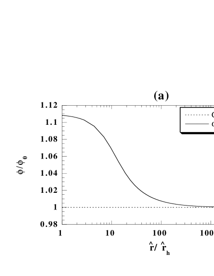
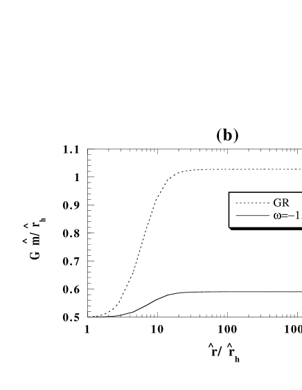
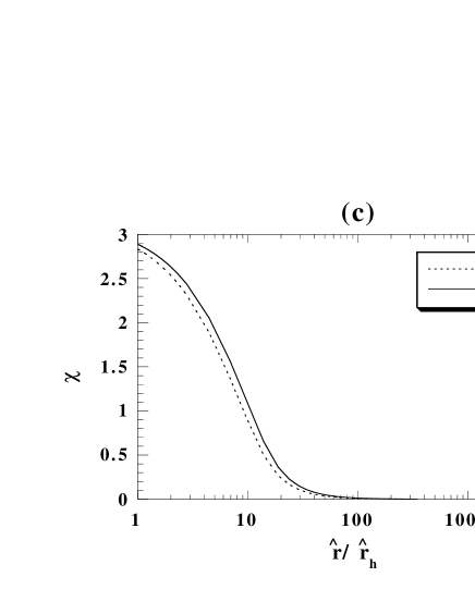
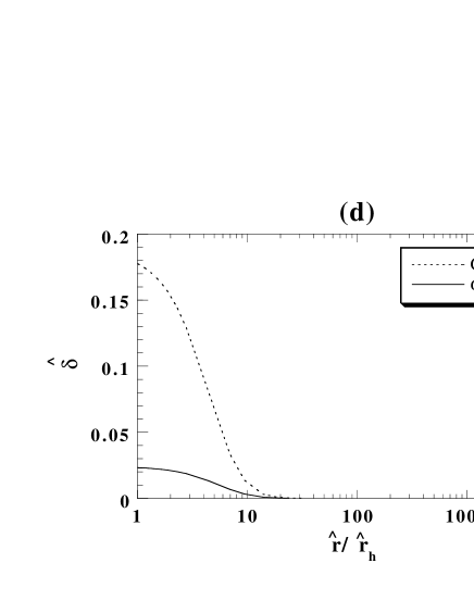
FIG. 19.: The solution of the Skyrme black hole with $\hat{r}_{h}=1.0l_{p}/g_{c}$ and $f_{s}=0.03m_{p}$ in BD theory ( (a) $\phi(r)$, (b) $\hat{m}(r)$, (c) $\chi(r)$, (d) $\hat{\delta}(r)$ ). : The Skyrme black hole in GR is also depicted as a reference.

Here we set the parameters as

$$\hat{r}_{h}=1.0l_{p}/g_{c},\ \ f_{s}=0.03m_{p},\ \ \omega=-1.4\ .$$ (68)

The dotted lines are those in GR with $\hat{r}_{h}=1.0l_{p}/g_{c}$ and $f_{s}=0.03m_{p}$. The solutions correspond to solid-line in Fig.20. We have shown only for a solution with one node number. For a Skyrme black hole, rather than the node number, the solution is characterized by the “winding” number defined by

$$W_{n}\equiv\frac{1}{\pi}|\chi_{h}-\chi(\infty)-\sin(\chi_{h})|\ .$$ (69)

We show for a solution with the “winding” number one. Note that the comparison is made in the Einstein frame for a fixed $\hat{r}_{h}$, which does not mean the horizon radii with different $\omega$ in the BD frame are the same.

$\hat{\delta}$ falls faster than $\hat{r}^{-1}$ because (59) is

$$\frac{d\hat{\delta}}{d\hat{r}}\sim-4\pi\hat{r}\left(\frac{d\varphi}{d\hat{r}}\right)^{2}\ ,$$ (70)

as $\hat{r}\rightarrow\infty$ and $\varphi$ vanishes faster than $\hat{r}^{-1}$ (see Figs.19(a), (d)). Then, as in the Proca black hole, $\hat{M}=\hat{M}_{g}$.

To study the properties of a family of black holes, we depict the $\hat{M}_{g}$-$\hat{r}_{h}$ and $M_{g}$-$r_{h}$ (the BD frame) diagrams in Fig.20 and the $M_{g}$-$1/T$ and $\hat{M}_{g}$-$1/T$ diagrams in Fig.21.

FIG. 20.: (a) $M_{g}$-$r_{h}$ diagram in the BD frame and (b) $\hat{M}_{g}$-$\hat{r}_{h}$ diagram in the Einstein frame for Skyrme black holes. We set $f_{s}=0.03m_{p}$.

FIG. 21.: (a) $M_{g}$-$1/T$ diagram in the BD frame and (b) $\hat{M}_{g}$-$1/T$ diagram in the Einstein frame for Skyrme black holes. We set $f_{s}=0.03m_{p}$.

We find that the results are quite similar to those for the Proca black holes. We have a cusp structure in the $\hat{M}_{g}$-$\hat{r}_{h}$ diagram in the Einstein frame, but it disappears in the BD frame.

Most properties found for the Proca black hole apply to the Skyrme black hole as well. This suggests that a universal picture for non-trivial black holes with massive non-Abelian fields is possible.

VII Concluding Remarks

We have analyzed non-Abelian black holes (Proca and Skyrme black holes) in BD theory and shown some differences from those in GR. The Einstein conformal frame makes our analysis easier. The effect of the BD scalar field can be reduced into two parts in the Einstein frame: the effective change of mass of the non-Abelian field, i.e. $\mu\rightarrow\mu\exp(-\kappa\beta\varphi/2)$ or $f_{s}\rightarrow f_{s}\exp(-\kappa\beta\varphi/2)$, and the renormalized coupling $g_{c}\rightarrow\sqrt{\phi_{0}}g_{c}$ or $g_{s}\rightarrow\sqrt{\phi_{0}}g_{s}$ and $f_{s}\rightarrow f_{s}/\sqrt{\phi_{0}}$. As a result, the solutions shift in the left-upper direction in the $M_{g}$-$r_{h}$ diagram. Although we recover the Schwarzschild black hole in the limit of $\omega\rightarrow-\frac{3}{2}$ in the Einstein frame, we still have non-trivial black holes in the BD frame in the same limit, because the conformal transformation becomes singular then.

Secondly, we have analyzed for various values of $\omega$. When $\omega\geq 500$, the difference from GR is so small that we will not see any observational difference. The solutions for $-\frac{3}{2}\leq\omega\mbox{\raisebox{-4.30554pt}{$\stackrel{{\scriptstyle\textstyle<}}{{\textstyle\sim}}$}}-1$ seem to be somewhat pathological, because the mass function $m$ becomes negative in the BD frame, resulting in negative value of $M$. However, even in such cases, $M_{g}$ is always positive, therefore a test particle around such a black hole still feels an attractive force.

Thirdly, we find that the cusp structure in $M_{g}$-$r_{h}$ diagram does not appear in the BD theory although it was found in GR and provided us a new method for stability analysis via catastrophe theory, while it exists in the Einstein frame. This suggests that a stability change occurs at a cusp point in the Einstein frame. The justification of this conjecture and the proper analysis including that by linear perturbations will be given elsewhere[14].

In this paper, we have studied a globally neutral type of non-Abelian black holes in BD theory. A globally charged black hole, i.e., a monopole black hole may be much more interesting. That is because charged black holes are important in the context of cosmology, in particular, in the relation with a dynamical monopole (topological inflation)[16]. This is under investigation.

ACKOWLEDGEMENTS

We would like to thank Jun-ichirou Koga for useful discussions and P. Haines for his critical reading. T. Torii is thankful for financial support from the JSPS. This work was supported partially by a Grant-in-Aid for Scientific Research Fund of the Ministry of Education, Science and Culture (Specially Promoted Research No. 08102010 and No. 09410217), by a JSPS Grant-in-Aid (No. 094162), and by the Waseda University Grant for Special Research Projects.