BROWN-HET-1096

We study the back reaction of cosmological perturbations on the evolution of the universe. The object usually employed to describe the back reaction of perturbations is called the effective energy-momentum tensor (EEMT) of cosmological perturbations. In this formulation, the problem of the gauge dependence of the EEMT must be tackled. We advance beyond traditional results that involve only high frequency perturbations in vacuo[1], and formulate the back reaction problem in a gauge invariant manner for completely generic perturbations. We give a quick proof that the EEMT for high-frequency perturbations is gauge invariant which greatly simplifies the pioneering approach by Isaacson[1]. As applications we analyze the back reaction of gravitational waves and scalar metric fluctuations in Friedmann-Robertson-Walker background spacetimes. We investigate in particular back reaction effects during inflation in the Chaotic scenario. Fluctuations with a wavelength much bigger than the Hubble radius during inflation contribute a negative energy density, and in that case back reaction counteracts any pre-existing cosmological constant. Finally, we set up the equations of motion for the back reaction on the geometry and on the matter, and show how they are perfectly consistent with the Bianchi identities and the continuity equations.

Chapter 1 Introduction

It is a well-known fact in oceanography that waves in the sea carry some amount of energy, which is released in the form of thermal energy as the waves crash on continental shorelines. This energy is responsible for a small fraction of the total thermal energy stored in the oceans’ water. Since waves pass through each other without much dispersion, the problem of propagation of sea waves can be treated linearly, and in fact oceanography analyses the several different classes of waves (of different amplitudes and wavelengths) independently from each other. Waves “average to zero” in the sense that the overall sea level, for a constant amount of water, is set at $0$ meters. Nevertheless, the average energy stored in waves is not zero, since it is not a linear but really a quadratic function of the wave. This second order phenomenon is the simplest case of a nonlinear feedback effect, or back reaction, in fluid dynamics.

A close analogy can be drawn between sea waves (called, ironically, “waves of gravity” in oceanographic jargon) and the coupled matter and metric perturbations (gravitational perturbations for short) with which we will concern ourselves here. The sea level and the temperature of the sea water correspond, respectively, to the background geometry upon which the waves (gravitational perturbations) propagate, and their energy density; the average of a gravitational perturbation is zero as well; the problem of propagation of perturbations can be treated in linear theory as a first approximation, although the exact problem, like fluid dynamics, is fundamentally nonlinear; the energy stored in the gravitational perturbations is, similarly, a quadratic function of the perturbations; finally, metric and density perturbations can effect the background geometry and energy density in which they propagate.

The theory of General Relativity[2, 3, 4], used here to describe gravitational systems, is much more complex than fluid dynamics in that one of its key elements is covariance under general gauge transformations that change the coordinate frames of observers in the manifold spacetime. Although this constraint on Einstein’s equations can be dealt with in exact problems containing symmetries and even in the linear theory of perturbations, to second order (when the quadratic effects associated with the energy carried by the waves appear), a formalism appropriate to the situation at hand has been sorely lacking in the literature. Consequently, many difficulties arise in the treatment of problems related to back reaction such as long calculations, lack of well-defined physical observables and, gravest of all: gauge dependence of the source of back reaction effects (which would correspond to the sea temperature), called the effective energy-momentum tensor of gravitational perturbations.

We separate gravitational perturbations in two broad classes: fluctuations which are of short wavelength and high frequency (HF), and the ones which have long wavelength and low frequency (LF). Although the problems cited above have been partially solved in the case of HF perturbations[1], we will see that, quite surprisingly, the decisive contribution from back reaction in at least one case (the Chaotic Inflationary scenario[5]) comes actually from the soft LF perturbations, and not from the hard HF ones.

We will show how a crucial ingredient in solving these problems is the fact that even linear gauge transformations (i.e., transformations that simply redefine the perturbations of matter and metric) can change the characteristics of the background geometry, as well as its dynamics. With that element in hand, we will show how it is possible to construct physical observables (gauge invariant quantities) which measure the effects of the back reaction of gravitational perturbations.

We apply this formalism to the problems of back reaction of gravitational waves (metric perturbations which are decoupled from matter sources) and scalar perturbations (coupled matter and metric fluctuations) in homogeneous and isotropic Friedmann-Robertson-Walker (FRW) background geometries. One of the results is that, due to back reaction, the equation of state of long wavelength gravity waves suffers corrections that have not been included in previous treatments.

The main result of our analysis comes from an application to the case of scalar perturbations during inflation in the chaotic model, where we have shown that back reaction can reduce the speed and the duration of inflation. The power of the feedback effects comes not from the amplitude of the perturbations, which is always small, but from the fact that the expansion of the universe redshifts the physical wavelengths of perturbations causing an exponential growth of the population of soft infrared (IR) modes.

As a spinoff of these ideas we suggest that back reaction might provide a dynamical relaxation mechanism whereby a preexisting cosmological constant is screened.

This work is organized as follows: in Chapter 2 we treat the problem of propagation of coupled metric and matter perturbations in FRW spacetimes, with special care given to the simple but interesting case of scalar field matter. Chapter 3 deals with the Chaotic Inflationary scenario, and with the process of generation of cosmological perturbations by quantum fluctuations of the scalar field. These introductory chapters can be skipped if the reader is familiar with modern cosmology.

We give a brief historical account of early as well as recent attempts to tackle the back reaction of gravitational perturbations in Chapter 4, and show how the problem in the context of HF perturbations can be formulated in a simpler way than before. In Chapter 5 we discuss the theory of finite gauge transformations, which we argue is fundamental to an understanding of some conceptual as well as practical issues related to back reaction. We also provide a covariant formulation of back reaction in generic backgrounds. Finally, in chapters 6 and 7 we develop applications to the case of gravity waves and scalar perturbations.

Chapter 2 The Theory of Cosmological Perturbations

Recent years have seen a confirmation of the basic working hypotheses of Cosmology: 1. that the universe is approximately homogeneous, with small perturbations superimposed onto this smooth background, and 2. that the universe is expanding, its energy density falling, and the temperature of the primordial background radiation is decreasing. The COBE satellite[6] and a series of similar experiments[7] have determined this fact beyond any dispute, and now it is finally clear that the plasma that predominated in the universe up to some $300,000$ years after the Big Bang was extremely homogeneous, in fact its temperature did not vary more than one part in $10^{5}$.

The structures on large scales that we see with the help of telescopes today (planets, clouds, galaxies, clusters of galaxies and so on) are but the result of a few billion-years of clumping of these tiny inhomogeneities in the plasma. The theory of the origin and evolution of these cosmological perturbations has become a cornerstone of modern cosmology, since by virtue of the theory of cosmological perturbations it is finally becoming possible to falsify models of the evolution of the early universe, as well as to test some of the underlying tenets of relativistic cosmology. The observation of the cosmic background radiation anisotropies, together with the theory of their origin and evolution, provides the matrix on which the basic parameters of cosmology (expansion rate, density, ratio of baryonic matter to total matter, deacceleration parameter and so on) have to be fitted.

Having established the importance of the study of perturbations in cosmology, it is to this we now turn.

2.1 Gravitational instability

Soon after publishing his seminal paper on General Relativity, Einstein used his theory to try and describe the Cosmos. It is important to notice that by 1917, when he published his “Kosmologische Betrachtungen zur allgemeinen Relativitätstheorie”[8], E. Hubble had not yet established Slipher’s suggestion that distant galaxies are receding, and therefore as far as anyone was concerned the Universe was static. Einstein soon realized that his theory would not lead to such a static Universe, and in order to achieve that he introduced a “universal constant”, now widely known as the cosmological constant $\Lambda$. In the ensuing model, a closed universe is kept static by the repulsive gravitational force coming from a fine-tuned cosmological constant. It just turns out that this model is unstable: it would expand (collapse) at an accelerated rate if the matter was slightly less (more) dense than some critical density.

The recent history of large-scale structure in the Universe is dominated by a similar type of gravitational instability: galaxies, for example, formed from gas clouds that collapsed by gravitational attraction around the galactic center. By the same process, smaller (stars, planets) and bigger (clusters and superclusters) structures also formed from this coarsening of a quasi-homogeneous expanding fluid. An evolution scenario that starts by forming the largest structures first is known as “top-down”, while one in which the small structures form first is known as “bottom-up”. The intermediate picture, of “scale-invariant” evolution, is the one that is currently favored by experimental data.

In the same manner that an overdensity is unstable to gravitational attraction and can grow to become a galaxy, for example, underdensities are also unstable and grow with time to form voids, regions with a much lower density of galaxies. In that case it is useful to think of an “effective gravitational repulsion”[9] acting on the matter in the boundaries between the voids, and pushing them together into pancakes. It is not clear which are the structures that dominate the Universe at the present time, but it has been argued that in the scale of clusters of galaxies, voids are in fact more pervasive than clusters[9].

Perturbations in the homogeneous fluid of a static Universe, as often happens with instabilities in Partial Differential Equations, grow in amplitude exponentially (their physical size of course grows together with the expansion of the Universe). If the expansion rate of the Universe is a power-law in time, i.e., if the physical scales $R\sim t^{m}$, the expansion counteracts the gravitational attraction and the perturbations’ amplitudes now grow only as a power-law: $\delta q\sim t^{n}$. Finally, if the universe is expanding exponentially (as it does if a cosmological constant dominates the evolution), perturbations are asymptotically static, that is, their amplitude tends to a constant.

Since the Universe at the present time seems to be expanding as a power-law, we conclude that it is also slowly becoming more and more complex, with growing voids and clusters of galaxies. But if there was a time when the Universe inflated exponentially, then perturbations with large enough wavelengths $\lambda>R_{H}$ would have been frozen during this period. If by some mechanism perturbations of that scale were created with the same amplitude during an inflationary phase, once that phase was over and a power-law expansion subsided the perturbations could then grow and start forming stars, galaxies, voids, etc. The spectrum of perturbations, that is, the amplitude of each mode with physical wavelength $\lambda$, would then be “scale-invariant”, which is consistent with the data available now.

In mathematical language, we will solve Einstein’s theory linearized around an expanding homogeneous background geometry[2, 3, 4]. A crucial issue is related to the freedom of gauge, that is, the symmetry under general coordinate transformations. It turns out that it is possible to build variables which have the same value in all coordinate frames, i.e., gauge-invariant variables, and those are of course the physically meaningful quantities. In the next sections we consider this theory in more detail.

2.2 Relativistic cosmology: background models

Clearly a Newtonian approximation to the description of the Universe in its largest scale is insufficient: since the expansion rate is now $65\pm 15kms^{-1}Mpc^{-1}$ (see [12] for an account of the latest measurements), galaxies at a distance of $1000Mpc$ from the Milky Way, for example, are receding from us at $20\%$ of the velocity of light. The expansion rate gets even bigger as we look back into the past, thus only Einstein’s relativistic theory is capable of providing an accurate description.

In a perfectly homogeneous and isotropic Universe, there are no preferred directions or axes in space, and the geometry, the metric and all other physical parameters depends only on time. We write the line element in this “cosmic time” as

$$ds^{2}=dt^{2}-a^{2}(t)d\vec{x}^{2}\quad,$$ (2.1)

where $a(t)$ is the scale factor. The spatial coordinates $\vec{x}$ are called “comoving coordinates”, and are related to physical distances by $\vec{r}=a(t)\vec{x}$ , hence the name “scale factor”. If we could sprinkle dots over the universe, the physical distances between dots would increase if the Universe was expanding and decrease if the Universe happened to be contracting, but the comoving distances between dots would nevertheless remain always the same. Eq. (2.1) is known as the Friedmann-Robertson-Walker (FRW) metric on flat space (we will not discuss here the trivial but cumbersome cases of open and closed Universes)

It will be practical, in certain applications, to use a different clock or time-slicing, where the time variable (called “conformal time”) is $d\eta=dt/a(t)$ . In this case we can write the line element as

$$ds^{2}=a^{2}(\eta)(d{\eta}^{2}-d\vec{x}^{2})\quad.$$ (2.2)

The time derivative of a function $f$ with respect to conformal time, $f^{\prime}$, can be related to the derivative with respect to cosmic time, $\dot{f}$, using the rule

$$\frac{d}{d\eta}f=a(t)\frac{d}{dt}f\quad.$$ (2.3)

The reader can freely exchange between the cosmic and conformal time pictures at any time.

The equations determining the kinematics and the dynamics of matter in General Relativity are the Einstein Field Equations,

$$G_{\mu\nu}=T_{\mu\nu}$$ (2.4)

where $G_{\mu\nu}$ is the Einstein tensor (which expresses a curvature of spacetime) and $T_{\mu\nu}$ is the energy-momentum tensor (EMT) of matter.

We will later consider more extensively the case of scalar field matter, where the EMT is given by

$$T_{\mu\nu}^{S}=\varphi_{,\mu}\varphi_{,\nu}-g_{\mu\nu}\left[\frac{1}{2}\varphi^{,\alpha}\varphi_{,\alpha}-V(\varphi)\right]\quad,$$ (2.5)

where $V(\varphi)$ is the potential of the scalar field $\varphi$.

For now, let us examine the more common cases of hydrodynamical fluids such as pressureless matter (dust) and radiation, whose EMTs can be expressed as

$$T_{\mu\nu}=\left(\begin{array}[]{cccc}\rho&0&0&0\\ 0&p&0&0\\ 0&0&p&0\\ 0&0&0&p\end{array}\right)$$ (2.6)

where $\rho(t)$ is the energy density, and the pressure $p(t)$ is related to the energy density by the equation of state $p=w\rho$ with $w$ constant. For matter we have $w_{d}=0$, while for radiation $w_{r}=1/3$. It is useful to note that when the dominant component of the Universe is a cosmological constant, the EMT can also be written as in (2.6), with $w_{\Lambda}=-1$.

In the homogeneous and isotropic background of a FRW Universe, with metric (2.2), the field equations (2.4) are diagonal and the time-time and space-space parts read, respectively,

$$3H^{2} = \rho\quad,$$ (2.7)

$$-3H^{2}-2\dot{H} = p$$ (2.8)

where $H=\dot{a}/a$ is the Hubble parameter, which measures the expansion rate of the universe. The inverse of the Hubble parameter $H^{-1}$ has dimensions of time, and is in fact a fundamental time scale in cosmology, since it is proportional to the age of the Universe - around 14 billion years, give or take a couple of billion years.

The geometric fact expressed by the Bianchi identities, $G_{\mu\nu}^{;\mu}=0$ is reciprocated on the rhs of (2.4) by the continuity equations, $T_{\mu\nu}^{;\mu}=0$ (semi-colons denote covariant derivative). The continuity equations are expressed, in a FRW Universe, by the constraint

$$\dot{\rho}+3H(\rho+p)=0\quad.$$ (2.9)

It is easy to see that the identity above is just the integrability condition that must be satisfied in order that Eqs. (2.7) and (2.8) have a solution. We can find the first integral of (2.9), which is

$$\rho\sim a(t)^{-3(1+w)}\quad.$$ (2.10)

Pressureless matter will have an energy density inversely proportional to the volume $V^{-1}\sim a^{-3}$, while radiation is not only diluted but also suffers from redshift, $\lambda_{ph}=\lambda/a(t)$, thus its energy density is proportional to $a^{-4}$. The temperature in radiation is related to its energy density by statistical mechanics, $\rho_{r}\sim T_{r}^{4}$, and thus $T_{r}\sim a^{-1}$. A cosmological constant ($w_{\Lambda}=-1$) have constant energy density. An important consequence of these equations is that, as we run the clock backwards (thus decreasing $a$), the energy density of radiation ( $\sim a^{-4}$ ) increases more rapidly than the one in matter ($\sim a^{-3}$) while the energy density due to a cosmological constant stays constant. We thus conclude that no matter how small the energy density in radiation is right now, it will necessarily be dominant in the early Universe.

Substituting the above expression into Eq. (2.7) yields the solution for the scale factor as a function of time,

$$a(t)\sim t^{\frac{2}{3(1+w)}}$$ (2.11)

if $w\neq-1$ and

$$a(t)\sim e^{H_{0}t}$$ (2.12)

if $w=-1$. In this last case, called de Sitter spacetime, the scale factor grows exponentially and the Hubble parameter is a constant, as evident in Eq. (2.7) . The fact that for non-exotic matter (such as a cosmological constant) the scale factor goes to zero when $t\rightarrow 0$ is an intrinsic feature of General Relativity, and this special case of space-like singularity is called the Big Bang.

At the present time the Universe is dominated by pressureless matter, with a fraction ($10^{-4}$) of the energy density contained in a background of photons which occupy the microwave band with a temperature of $2.73^{\circ}K$ (thus the name Cosmic Microwave Background Radiation - CMBR). Approximately 1,000,000 years after the Big Bang, though, the energy density is still just high enough that the temperature of the CMBR can ionize Hydrogen atoms. After this moment (sometimes also called recombination), when $T_{dec}\approx 3000^{\circ}K$, matter becomes transparent to radiation and they decouple from each other.

An important consequence of recombination is that photons did not scatter from matter after the time of decoupling $t_{dec}$ up to the present time. In other words, they traveled in a straight line since this “surface of last scattering” at $t_{dec}$ (see Fig. 2.1), and if we can set the temperature of our experiment low enough that we can detect those photons, we will be seeing a picture of the last events that took place at this time of decoupling.

Figure 2.1: Surface of last scattering (dotted circle) of the cosmic microwave background radiation. Photons that emerged from overdense regions after the time of decoupling are more redshifted then photons that came from underdense regions.

That is the content of the map of the CMBR sky produced by the COBE satellite. Photons coming from the surface of last scattering have an average temperature of $2.736^{\circ}K$, with fluctuations in the quadrupole of about one part in $5\times 10^{-6}$, or $10mK$. There is also a dipole that was subtracted in the CMBR map which is ascribed to a peculiar motion of our galaxy, with respect to this “ether” of primordial photons, of about $370$ $km$ $s^{-1}$.

Notice that the presence of this background of radiation introduces a class of preferred reference frames (coordinates) for observers in the Universe: the comoving observers. It would make little sense to utilize a reference frame which is moving with respect to the background photons, since it would introduce dipoles in the CMBR, in the Hubble diagrams, and indeed in most all-sky observations.

It is important to stress this fact: when talking about cosmology, we are going to consider only reference frames (or coordinate frames) which are, within a first approximation, static with respect to the cosmic background radiation. When we consider gauge transformations, in this context, we will be always considering transformations between coordinate frames inside this class of quasi-static comoving frames. A precise mathematical formulation of this point will be given in Section 5.1.

Before concluding this section let us examine the important case of scalar field matter, which will be crucial in the next sections. If the Universe is filled with a homogeneous scalar field $\varphi_{0}(t)$ with potential energy $V(\varphi_{0})$, the EMT is diagonal with energy density and pressure given by

$$\rho_{s}=\frac{1}{2}\dot{\varphi}_{0}^{2}+V(\varphi_{0})\quad,$$ (2.13)

$$p_{s}=\frac{1}{2}\dot{\varphi}_{0}^{2}-V(\varphi_{0})\quad.$$ (2.14)

When the potential term dominates, the EMT is identical to the EMT of a cosmological constant $\Lambda=V(\varphi_{0})$. If such a scalar field is dominant over other forms of matter, the Universe will expand exponentially - or inflate - like de Sitter space, until the kinetic terms become comparable to the potential term. If this inflationary period lasts long enough, an apparent event horizon is created due to the exponentially fast expansion rate. Two observers in opposite poles of a sphere with radius the size of the horizon $R_{H}$ will not be able to exchange signals, because the expansion of the Universe is so fast that those signals cannot reach the other poles. Of course, once inflation is over those signals can progress towards the other observer once again, but during inflation we can define this horizon. Clearly, the faster the expansion rate the smaller the horizon size, and in fact, $R_{H}=H^{-1}$. The existence of horizons during periods of quasi-exponential expansion will be a welcome feature of inflationary models that we explore later on.

In many situations (during the reheating phase after inflation, for example) the scalar field is oscillating coherently around the zero of the potential with amplitude $2{\bar{\varphi}}_{0}$, and then on average the kinetic term equals the potential term, implying that $\bar{p}_{s}=0$ and $\bar{\rho}_{s}=2V(\bar{\varphi}_{0})$.

The continuity equations in the case of scalar field matter are just the equation of motion for $\varphi_{0}$ (the Klein-Gordon equation in a FRW spacetime) and read

$$\ddot{\varphi}_{0}+3H\dot{\varphi}_{0}+V_{,\varphi}(\varphi_{0})=0\quad.$$ (2.15)

In general the first situation described above (potential energy dominance) implies that the first term in (2.15) can be neglected. In that case $\dot{\varphi}_{0}\cong-V^{\prime}/3H$ and the scalar field is “slowly rolling” down towards the minimum of the potential. The second situation (coherent oscillations) usually means that the friction term $3H\dot{\varphi}_{0}$ is negligible.

We conclude then that if the Universe was initially dominated by a scalar field displaced from the zero of its potential, it would inflate exponentially until the friction term became small, and then it would expand in a power-law just like in a matter-dominated Universe with $p_{s}=0$.

2.3 Perturbations of FRW spacetimes

The mosaic of hot and cold spots in the COBE map of the CMBR shows that some regions of the early Universe were slightly hotter (and therefore denser) than others. Since energy curves space, this implies that the metric was also largely homogeneous, with some small bumps corresponding to the hot and cold spots. Call $\epsilon$ the adimensional measure of the magnitude of these inhomogeneities. In the case of our Universe at the time of decoupling, $\epsilon$ is, explicitly,

$$\epsilon_{dec}=\left.\frac{\delta T}{T}\right|_{dec}\approx 10^{-5}\quad,$$ (2.16)

where $\delta T$ denotes the fluctuations in the temperature field. Metric perturbations can be preliminarily thought of as proportional to the variation of the newtonian potential, which in turn is proportional to the temperature fluctuations of the primordial plasma. The constant $\epsilon$ thus regulates the size of both matter and metric perturbations, and in fact can even be related to the small parameter that enters when we consider gauge transformations (see next section).

Although the background variables depend only on the coordinate $\eta$ (we use conformal time here for convenience) the perturbed variables can vary along all the 4 coordinates. The scalar field, thus, will be written as

$$\varphi=\varphi_{0}(\eta)+\epsilon\delta\varphi(\eta,\vec{x})\quad,$$ (2.17)

and the metric $g_{\mu\nu}$ as

$$g_{\mu\nu}=\gamma_{\mu\nu}(\eta)+\epsilon\delta g_{\mu\nu}(\eta,\vec{x})$$ (2.18)

where $\gamma_{\mu\nu}$ is given in (2.2),

$$\gamma_{\mu\nu}=a^{2}(\eta)\left(\begin{array}[]{ll}1&0\\ 0&-\delta_{ij}\end{array}\right)\quad.$$ (2.19)

The metric perturbations $\delta g_{\mu\nu}$ of a homogeneous and isotropic background (2.19) can actually be classified into scalar, vector and tensor, each category belonging to different “multiplets” of the group of spatial coordinate transformations on a fixed time slice (for a review, see [13]). Scalar perturbations transform between each other when the coordinate transformation can be expressed in terms of a 3-scalars; vector perturbations mix with other vector perturbations when the transformation is due to a traceless 3-vector; and tensor perturbations (also known as gravitational waves) are unchanged since there is no way by which a genuine traceless, divergenceless 3-tensor can produce a coordinate transformation. We will concern ourselves mostly with scalar and tensor perturbations, since in most applications vector perturbations decay rapidly. As would be expected, each perturbative “mode” couple to different sectors of matter, in such a way that there is no correlation between the 3 categories, and we can analyze them separately.

The scalar perturbations can be constructed in terms of 4 scalar quantities, $\phi$, $\psi$, $B$ and $E$:

$$\delta g_{\mu\nu}^{S}=a^{2}(\eta)\left(\begin{array}[]{ll}2\phi&-B_{,i}\\ -B_{,j}&2[\psi\delta_{ij}-E_{,ij}]\end{array}\right)\quad.$$ (2.20)

Vector perturbations can be written in terms of two transverse (or solenoidal) 3-vectors $S_{i}$ and $F_{i}$ (if they were not transverse we could extract scalars - the divergences $S^{i}_{,i}$ and $F^{i}_{,i}$ - from them and construct new, transverse vectors)

$$\delta g_{\mu\nu}^{V}=-a^{2}(\eta)\left(\begin{array}[]{ll}0&-S_{i}\\ -S_{j}&F_{i,j}+F_{j,i}\end{array}\right)\quad.$$ (2.21)

Finally, tensor perturbations can be cast in terms of a traceless, transverse 3-tensor $h_{ij}$. Again, if the constraints $h^{i}_{i}=0$ or $h^{i}_{j,i}=0$ were not satisfied, we could extract a scalar or a vector from $h_{ij}$ and then construct a new tensor that would be traceless and transverse. The metric perturbations for gravitational waves are thus

$$\delta g_{\mu\nu}^{T}=-a^{2}(\eta)\left(\begin{array}[]{ll}0&0\\ 0&h_{ij}\end{array}\right)\quad.$$ (2.22)

The accounting for degrees of freedom is the following:

4 d.o.f. for scalar modes (0 constraints);

4 d.o.f. for vector modes (2 constraints);

2 d.o.f. for tensor modes (4 constraints),

giving a total of 10, which is the number of independent components of the symmetric tensor $\delta g_{\mu\nu}$.

The splitting above, into scalar, vector and tensor modes, is specific to the FRW background, and would not be valid if the 3-space was not homogeneous and isotropic. In the case when the background is a Schwarzschild geometry, which is symmetric on two of the variables (the polar and azimuthal angles) but not on the radius, perturbations can be separated into similar groups that transform according to rotations in $S^{2}$.

2.4 Diffeomorphism transformations

General Relativity is a diffeomorphism-invariant theory, i.e., its action and physical observables are symmetric under transformations that take any one coordinate frame continuously into another. A general infinitesimal coordinate transformation takes a system of coordinates $\{x^{\mu}\}$ of a given manifold ${\cal M}$ into a different coordinate system $\{\tilde{x}^{\mu}\}$ in such a way that the structure of the manifold remains the same. This mathematical definition means that physically meaningful observables such as the topology, the existence of singularities or the amplitude of the quadrupole anisotropy in the CMBR are notions which are independent of the coordinate frame we happen to choose.

In infinitesimal form, we can write a general gauge transformation as

$$x^{\mu}_{P}\longrightarrow\tilde{x}^{\mu}_{P}=x^{\mu}_{P}+\varepsilon\xi^{\mu}_{P}\quad,$$ (2.23)

where $\varepsilon$ is a small parameter (later $\varepsilon$ will be identified with the $\epsilon$ that measures the relative magnitude of perturbations) and $\xi(x)$ is a general 4-vector. Here we present a simplified version of the treatment given in Chapter 5. For a fuller discussion of the issue of perturbations of homogeneous spacetimes, see [14] and [15]

Now the question is, how do tensors transform under a gauge transformation? In fact tensors by definition transform according to the law

$$q^{\mu\cdots}_{\nu\cdots}(x_{P})\rightarrow{\tilde{q}}^{\mu\cdots}_{\nu\cdots}(\tilde{x}_{P})={\partial\tilde{x}^{\mu}\overwithdelims( )\partial x^{\alpha}}_{P}\cdots{\partial x^{\beta}\overwithdelims( )\partial\tilde{x}^{\nu}}_{P}\cdots q^{\alpha\cdots}_{\beta\cdots}(x_{P})\quad.$$ (2.24)

Notice that on the l.h.s. of this equation the components $\tilde{q}$ are evaluated at the coordinate value $\tilde{x}^{\mu}_{P}=x^{\mu}_{P}+\varepsilon\xi^{\mu}_{P}$. Substituting this expression for $\tilde{x}$ into Eq. (2.24) and expanding both the left and the right-hand-sides yields the definition of the Lie derivative

$$\tilde{q}(x_{P})=q(x_{P})-\varepsilon{\cal L}_{\xi}q(x_{P})+{\cal O}(\varepsilon^{2})\quad.$$ (2.25)

The Lie derivative can be interpreted as being the differential operator that transforms tensors without changing the coordinate point at which the tensor is evaluated. We speak then of “Lie dragging” tensors over real points whose coordinate values have been fixed, along a line with tangent vector $\xi$. The difference between tensor components before and after the dragging defines the Lie derivative.

The algebraic definition of the Lie derivative is quite straightforward: it acts on 4-scalars as

$${\cal L}_{\xi}S=S_{,\alpha}\xi^{\alpha}\quad,$$ (2.26)

on vector fields as

$$\left({\cal L}_{\xi}v\right)^{\mu}=v^{\mu}_{,\alpha}\xi^{\alpha}-v^{\alpha}\xi^{\mu}_{,\alpha}\quad,$$ (2.27)

on 1-forms (covariant vectors) as

$$\left({\cal L}_{\xi}u\right)_{\mu}=u_{\mu,\alpha}\xi^{\alpha}+u_{\alpha}\xi^{\alpha}_{,\mu}\quad,$$ (2.28)

and so forth for higher-ranking tensors. The case of the metric tensor $g_{\mu\nu}$ is particularly important:

$$\tilde{g}_{\mu\nu}=g_{\mu\nu}-\varepsilon\left({\cal L}_{\xi}g\right)_{\mu\nu}=g_{\mu\nu}-\varepsilon g_{\mu\nu,\alpha}\xi^{\alpha}-\varepsilon g_{\alpha\nu}\xi^{\alpha}_{,\mu}-\varepsilon g_{\mu\alpha}\xi^{\alpha}_{,\nu}\quad.$$ (2.29)

A coordinate transformation that leaves the metric unchanged is called an isometry, and vector fields $\zeta$ (called Killing vectors) that generate isometries obey the Killing equations.

$$g_{\mu\nu,\alpha}\zeta^{\alpha}-g_{\alpha\nu}\zeta^{\alpha}_{,\mu}-g_{\mu\alpha}\zeta^{\alpha}_{,\nu}=-\zeta_{\mu;\nu}-\zeta_{\nu;\mu}=0\quad.$$ (2.30)

We want to argue now that, to our purposes, the small parameter $\varepsilon$ is the same as the $\epsilon$ introduced before as the measure of the strength of the perturbations in FRW spacetimes. As we discussed, we will be concerned only with coordinate frames which describe the Universe as approximately homogeneous and isotropic. This means that the background spacetime is constrained to be described by the metric (2.2) and the homogeneous scalar field $\varphi_{0}(\eta)$, up to a trivial time reparametrization. We can still allow, though, for coordinate transformations that change the form of the matter and metric perturbations $\delta\varphi$ and $\delta g_{\mu\nu}$. Equation (2.29) reads then

$$\tilde{g}_{\mu\nu} = \tilde{\gamma}_{\mu\nu}+\epsilon\delta{\tilde{g}}_{\mu\nu}=\gamma_{\mu\nu}+\epsilon\delta g_{\mu\nu}-\varepsilon\left[{\cal L}_{\xi}(\gamma+\epsilon\delta g)\right]_{\mu\nu}$$ (2.31)

$$= \gamma_{\mu\nu}+\epsilon\delta g_{\mu\nu}-\varepsilon\gamma_{\mu\nu,\alpha}\xi^{\alpha}-\varepsilon\gamma_{\alpha\nu}\xi^{\alpha}_{,\mu}-\varepsilon\gamma_{\mu\alpha}\xi^{\alpha}_{,\nu}+{\cal O}(\epsilon\varepsilon)\quad,$$

which after subtracting the background yields

$$\epsilon\delta{\tilde{g}}_{\mu\nu}(x)=\epsilon\delta g_{\mu\nu}(x)-\varepsilon\gamma_{\mu\nu,\alpha}\xi^{\alpha}(x)-\varepsilon\gamma_{\alpha\nu}\xi^{\alpha}_{,\mu}(x)-\varepsilon\gamma_{\mu\alpha}\xi^{\alpha}_{,\nu}(x)+{\cal O}(\epsilon\varepsilon)\quad.$$ (2.32)

The matter perturbations change similarly, and it is easy to see that

$$\epsilon\delta\tilde{\varphi}(x)=\epsilon\delta\varphi-\varepsilon\varphi_{,\alpha}\xi^{\alpha}(x)+{\cal O}(\epsilon\varepsilon)\quad.$$ (2.33)

From the equations above we can conclude that if the magnitude of perturbations is to be preserved under gauge transformations, then $\varepsilon\leq\epsilon$. In case of equality, the gauge transformation can potentially redefine the perturbations; if $\varepsilon\ll\epsilon$ the gauge transformations do not alter significantly the perturbations, and we can ignore their effect. We will use the saturated bound $\varepsilon=\epsilon$ and drop their distinction altogether, since we are interested in gauge transformations that are large enough that they actually affect the perturbations. Of course this upper bound constrains the class of gauge transformations that are allowed, but the price of not going along these lines is giving up a well-defined notion of background. In order not to make notation too heavy, we drop any reference to $\epsilon$, and without ambiguity assume it implicit in the definitions of $\xi$ and the perturbations.

If we separate the metric perturbations into the three categories described in the end of the last section (scalar, vector and tensor), gauge transformations do not destroy this classification. In a FRW background spacetime any 4-vector $\xi(\vec{x},\eta)$ can be decomposed in a 3+1 fashion into two 3-scalars and one transverse 3-vector,

$$\xi^{\mu}=\left[\xi^{0},\xi^{,i}_{s}+\xi^{i}_{T}\right]\quad,$$ (2.34)

where $\xi^{0}(\vec{x},\eta)$ and $\xi_{s}(\vec{x},\eta)$ are 3-scalars and $\xi^{i}_{T}(\vec{x},\eta)$ is a 3-vector such that $\xi^{i}_{T\,,i}=0$ .

Using the general coordinate transformations above, the metric perturbations $\delta g_{\mu\nu}^{S}+\delta g_{\mu\nu}^{V}+\delta g_{\mu\nu}^{T}$ given in (2.20)-(2.22) and the background metric (2.19) and substituting into Eq. (2.32) we find that metric perturbations change in the following way (a prime denotes derivative with respect to conformal time, $a^{\prime}=da/d\eta$): for scalar perturbations,

$$\phi\rightarrow\tilde{\phi} = \phi-\frac{a^{\prime}}{a}\xi^{0}-{\xi^{0}}^{\prime}\quad,$$ (2.35)

$$\psi\rightarrow\tilde{\psi} = \psi+\frac{a^{\prime}}{a}\xi^{0}\quad,$$ (2.36)

$$B\rightarrow\tilde{B} = B+\xi^{0}-{\xi_{s}}^{\prime}\quad,$$ (2.37)

$$E\rightarrow\tilde{E} = E-\xi_{s}\quad;$$ (2.38)

for the vector perturbations,

$$S^{i}\rightarrow\tilde{S}^{i} = S^{i}-{\xi^{i}_{T}}^{\prime}\quad,$$ (2.40)

$$F^{i}\rightarrow\tilde{F}^{i} = F^{i}-\xi^{i}_{T}\quad;$$ (2.41)

finally, the tensor perturbations (gravity waves), as we noted, do not transform,

$$h_{ij}\rightarrow\tilde{h}_{ij}=h_{ij}\quad.$$ (2.43)

On the other hand, matter perturbations are transformed according to their character: scalar field perturbations are simplest,

$$\delta\varphi\rightarrow\delta\tilde{\varphi}=\delta\varphi-\varphi_{0}^{\prime}\xi^{0}\quad.$$ (2.44)

Background 4-vector fields in homogeneous and isotropic spaces are such that their spatial components vanish (a non-vanishing component $v^{i}_{(0)}$ would define a preferred orientation and break isotropy), so $v^{\mu}_{(0)}=[v^{0}_{(0)}(\eta),0]$. Perturbations of vector fields in 3+1 can be decomposed into a transverse 3-vector field plus two scalar fields, $\delta v^{\mu}=[\delta v^{0},\delta v^{i}_{T}+\delta v^{,i}]$ and their components transform as

$$\delta v^{0} \rightarrow \delta\tilde{v}^{0}=\delta v^{0}-{v_{(0)}^{0}}^{\prime}\xi^{0}+v^{0}_{(0)}{\xi^{0}}^{\prime}\quad,$$ (2.45)

$$\delta v \rightarrow \delta\tilde{v}=\delta v+v^{0}_{(0)}{\xi^{0}}^{\prime}\quad,\quad{\rm and}$$ (2.46)

$$\delta v^{i}_{T} \rightarrow \delta\tilde{v}^{i}_{T}=\delta v^{i}_{T}+v^{0}_{(0)}{\xi^{i}_{T}}^{\prime}\quad.$$ (2.47)

This separation can be carried out to tensors of arbitrary rank.

Finally, let us comment on the problem of the “choice of gauge”. The metric tensor has 10 components, but due to the diffeomorphism symmetry, only 6 are truly dynamical variables. In order to “fix” a gauge we must impose constraints on the metric variables. From the definition of the diffeomorphism generator, Eq. (2.34), we draw that there are 2 constraints that can be imposed on the 4 scalar modes, and 2 that can be imposed on the 4 vector modes (the tensor modes are already properly constrained by the TT conditions). There are then 6 dynamical variables in the metric tensor: 2 scalar, 2 vector and 2 tensor modes.

We must stress that the constraints on the metric perturbations should completely remove the gauge freedom. Some gauge choices fail to do so (the synchronous gauge defined by the constraints $\delta g_{0\mu}=0$ is a typical example), and the price to pay for this shortcoming is having to deal with gauge modes that grow in time and obscure the calculation. We will work later with a gauge choice (longitudinal gauge) that eliminates completely the freedom under coordinate transformations.

2.5 Gauge invariant variables

The transformation laws for scalar, vectors and tensor perturbations show that they have distinct expressions in distinct reference frames. Now that we know how the gauge symmetry of gravity influences perturbations, we can try to find physical observables that can describe those perturbations in an invariant form. A quantity is said to be “gauge invariant” if it is independent of $\xi$ when the reference frame is transformed by $x\rightarrow\tilde{x}=x+\xi$. Geometric quantities such as tensors (scalars included) are covariant, not invariant, and are not included in this category.

However, Bardeen[18] was able to construct non-geometric quantities defined with respect to a particular coordinate frame, which take the same values in all nearby frames. An example of a non-geometric quantity would be the sum of a scalar with the $0-0$ component of a mixed tensor of rank $(1,1)$.

In this monograph we will follow a slightly distinct but equivalent construction than the one carried out in the standard references [13, 18, 19]. While this treatment is less straightforward, it will prove much more useful when we generalize gauge transformations in Chapter 5.

First, we note that $\xi$ is completely general, and that it has the same order of magnitude as the perturbations (the factor $\epsilon$ that we dropped earlier). We can choose its components $\xi^{0}$, $\xi_{s}$ and $\xi^{i}_{t}$ to be arbitrary functions in a particular frame. In particular we could choose them to be linear combinations of the components of the metric perturbations, and in fact that is what we should do if we would like to go to a frame where, e.g., $\tilde{E}=0$ : by Eq. (2.39) we easily see that we would have to make a gauge transformation with $\xi_{s}=E$.

Call $X^{\mu}[\delta g]$ the special kind of “vectors” defined in terms of the perturbations such that, under a gauge transformation,

$$X^{\mu}[\delta g]\rightarrow\tilde{X}^{\mu}[\delta\tilde{g}]=X^{\mu}[\delta g]+\xi^{\mu}\quad.$$ (2.48)

In other words, under a coordinate transformation generated by $\xi$, the vectors $X$ transforms like the coordinates. What we mean by (2.48) is that $X^{\mu}$ are linear functional of the components of the tensor $\delta g_{\mu\nu}$ which, under a gauge transformation, change in such a way that $\tilde{X}^{\mu}$, written in terms of $\delta{\tilde{g}}_{\mu\nu}$, is related to $X^{\mu}$ by (2.48).

Suppose now that we found at least one vector $X$ that conforms to our specifications. Consider then the following quantities $Q^{\mu\cdots}_{\nu\cdots}$ defined in terms of a generic tensor $q^{\mu\cdots}_{\nu\cdots}$ with the help of $X$:

$$Q\equiv q+{\cal L}_{X}q\quad.$$ (2.49)

If q has a perturbative expansion $q=q_{0}(\eta)+\delta q(\eta,\vec{x})$, then naturally the background is the same, $Q_{0}=q_{0}$, but not the perturbations:

$$\delta Q=\delta q+{\cal L}_{X}q_{0}\quad.$$ (2.50)

The transformation law for $\delta Q$ can be calculated as follows:

$$\delta\tilde{Q} = \delta\tilde{q}+{\cal L}_{\tilde{X}}q_{0}=\delta q-{\cal L}_{\xi}q_{0}+{\cal L}_{X+\xi}q_{0}$$ (2.51)

$$= \delta q+{\cal L}_{X}q_{0}=\delta Q\quad.$$

Therefore, the quantities $\delta Q=\delta\tilde{Q}$ are gauge invariant variables! It is possible then to define gauge invariant quantities related to the perturbations of any background variables, provided that we can find a vector $X$ that satisfies the transformation law (2.48).

With the help of the transformation laws for the metric perturbations it is easy to extract the components that transform in the desired way. Since there is more than one solution for each component $X^{0}$, $X_{s}$ and $X^{i}_{t}$, we label them as follows:

$$X^{0}_{(1)} = B-E^{\prime}\quad,$$ (2.52)

$$X^{0}_{(2)} = \frac{a}{a^{\prime}}\psi\quad,$$

$$X^{0}_{(3)} = -\int d\eta(\phi+\frac{a^{\prime}}{a}X^{0}_{(1,2)})\quad,$$

$$X_{S(1)} = -E\quad,$$

$$X_{S(2)} = -\int d\eta(B-X^{0})\quad,$$

$$X^{i}_{T(1)} = -F^{i}\quad,$$

$$X^{i}_{T(2)} = -\int d\eta S^{i}\quad.$$

In the definition of $X_{(3)}^{0}$ the last term can be any linear combination of $X_{(1)}^{0}$ and $X_{(2)}^{0}$ with norm 1 (see below).

For each one component we can actually use various definitions, as long as they sum up to unity. For example, we could define

$$X^{0}_{(\alpha)}=\frac{1}{4}X^{0}_{(1)}+\frac{3}{4}X^{0}_{(2)}\quad,$$

or

$$X_{S(\beta)}=0.78X_{S(1)}+0.22X_{S(2)}\quad.$$

There is an infinite number of definitions that we could choose, corresponding to an infinite number of ways of defining gauge invariant objects. We would prefer the simplest possible definition, that in addition is regular if we choose to switch off the expansion of the Universe and is not nonlocal (does not include integrals). We will also neglect the vector modes, since they do not play a significant role neither in structure formation nor in back reaction, which is the object of this work.

We are left with only one simple choice,

$$X^{0}=B-E^{\prime}\quad,$$ (2.53)

and

$$X_{s}\equiv X=-E$$ (2.54)

and, of course, $X^{i}_{T}=0$ since we are not going to allow for vector modes in any reference frame. With these definitions we can compute the explicit expressions for gauge invariant metric components. Substituting in Eq. (2.50) and separating the components we have

$$\phi \stackrel{{\scriptstyle X}}{{\rightarrow}} \Phi=\phi+\frac{1}{a}[a(B-E^{\prime})]^{\prime}\quad,$$ (2.55)

$$\psi \stackrel{{\scriptstyle X}}{{\rightarrow}} \Psi=\phi-\frac{a^{\prime}}{a}(B-E^{\prime})\quad,$$ (2.56)

$$B \stackrel{{\scriptstyle X}}{{\rightarrow}} 0\quad{\rm and}$$

$$E \stackrel{{\scriptstyle X}}{{\rightarrow}} 0\quad.$$

The gauge invariant variable related to the scalar field perturbation is also defined in Eq. (2.50),

$$\delta\varphi\quad\stackrel{{\scriptstyle X}}{{\rightarrow}}\quad\delta\varphi_{gi}=\delta\varphi+{\varphi_{0}}^{\prime}(B-E^{\prime})\quad.$$ (2.57)

While the construction detailed above is undeniably more involved than the one usually encountered in the literature, in the end of the day it proves simpler. The classical construction consists of looking for gauge invariant combinations of components of a given tensor with the metric perturbations. In our construction, once the $X$ are properly identified and classified (a trivial procedure), it is a matter of simple algebra to calculate the gauge invariant variables corresponding to any tensor. It will also prove much simpler to deal with once we go beyond the first order in perturbation theory in Chapter 5.

So far we did not impose any constraints on the metric, therefore the “gauge” is completely general. Since we have excluded the vector modes from the analyses (2 constraints), we still have to impose 2 conditions on the scalar functions. We could choose, for example, the synchronous gauge $\phi=0$ and $B=0$, but these 2 constraints are not sufficient to completely eliminate the gauge freedom (see [13]). We will use instead the constraints that make definitions (2.53) and (2.54) easiest to compute, i.e., $B=0$ and $E=0$, known as longitudinal gauge (since the metric perturbations are diagonal). There are three good reasons for this choice of gauge: one is that, as opposed to synchronous gauge, longitudinal gauge does not carry any “unphysical modes”, therefore we do not have to deal with “ghosts” in the calculation; two, $\phi$ can be connected to the gravitational potential in the Newtonian limit, and it is desirable that we can easily take that limit if we wish to; finally, in the gauge where $B=E=0$, the dynamical variables $\phi$ and $\psi$ actually coincide with the gauge invariant variables $\Phi$ and $\Psi$, respectively.

In fact, with the choice of the vector $X$ as in (2.53) and (2.54), all gauge-invariant variables are coincident with their expressions in longitudinal gauge. This suggests an elegant way of writing the equations for cosmological perturbations in a completely gauge invariant manner: we derive the equations of motion in longitudinal gauge, then substitute $\phi$, $\psi$ and $\delta\varphi$ for their gauge invariant counterparts $\Phi$, $\Psi$ and $\delta\varphi_{gi}$.

Since we are going to use the longitudinal gauge for the remainder of this paper whenever we speak of scalar perturbations, we can drop the notational distinction between the gauge invariant variables and their corresponding longitudinal gauge variables. Thus from now on we restrict ourselves to the scalar metric perturbations given by

$$\delta g_{\mu\nu}^{S}=a^{2}(\eta)\left(\begin{array}[]{ll}2\phi&0\\ 0&2\psi\delta_{ij}\end{array}\right)\quad.$$ (2.58)

It goes without saying that gravity waves do no interfere at all with the discussion above, since they are gauge invariant to start with.

2.6 Equations of motion for the perturbations

The propagation of linearized perturbations in a background spacetime is given by the Einstein field equations, expanded in a Taylor series around the background metric $\gamma_{\mu\nu}$ and matter fields $\varphi_{0}$, truncated at the second order. We will use the following notation:

$$0=G_{\mu\nu}[g]-T_{\mu\nu}[g,\varphi] \equiv \Pi_{\mu\nu}[g,\varphi]$$ (2.59)

$$= \left.\Pi_{\mu\nu}^{(0)}[\gamma,\varphi_{0}]+\delta\Pi_{\mu\nu}[\delta g,\delta\varphi]\right|_{\gamma,\varphi_{0}}\quad.$$

The tensor $\Pi_{\mu\nu}^{(0)}$ is zero if the background equations $G_{\mu\nu}^{(0)}=T_{\mu\nu}^{(0)}$ are satisfied, which of course must be solved prior to the linear equations $\delta G_{\mu\nu}=\delta T_{\mu\nu}$. It is straightforward but lengthy to derive the linearized equations of motion, and it is widely available in the literature[13]. We simply state here the results for the cases of gravity waves (tensor perturbations) and scalar perturbations. We neglect the vector modes, since they do not appear in most models of structure formation.

Einstein’s equations linearized around a FRW background spacetime imply the following equations of motion for the tensor modes:

$$h_{ij}^{\prime\prime}+2{\cal H}h_{ij}^{\prime}-\nabla^{2}h_{ij}=0$$ (2.60)

where ${\cal H}=a^{\prime}/a$ and a prime, as before, denotes a derivative with respect to conformal time. Notice that the right-hand-side of Eq. (2.60) does not contain any matter source, which is the reason why gravity waves do not couple to matter.

It is useful to make the substitution

$$h_{ij}(\vec{x},\eta)=\frac{1}{a(\eta)}\int\frac{d^{3}k}{(2\pi)^{3/2}}\left[\mu_{k}(\eta)\epsilon_{ij}(\vec{k})e^{i\vec{k}\cdot\vec{x}}+c.c.\right]\quad,$$ (2.61)

in which case the equations of motion for $\mu(\eta)$ read simply

$$\mu_{k}^{\prime\prime}+\left(k^{2}-\frac{a^{\prime\prime}}{a}\right)\mu_{k}=0\quad.$$ (2.62)

Due to the constraints on the tensor modes, $h^{i}_{i}=h^{i}_{j,i}=0$, the polarization tensor $\epsilon_{ij}$ in (2.61) is a symmetric and transverse-traceless (TT) tensor, $\epsilon^{i}_{j}=\epsilon_{ij}k^{i}=0$. Consider a gravity wave moving in the $z$ direction, that is, $\vec{k}=(0,0,k_{z})$. The constraints imply that the polarization tensor for this plane wave is given in terms of the two variables $\epsilon_{xx}=-\epsilon_{yy}$ and $\epsilon_{xy}=\epsilon_{yx}$. For each plane wave there are then 2 degrees of freedom, transverse to the direction of propagation of the wave.

When the background expands in time as $a\propto\eta^{p}$, the equation can be solved in terms of (spherical) Bessel functions:

$$\mu(k,\eta)=\eta^{1/2}\left[C_{1}(k)J_{p-1/2}(k\eta)+C_{2}(k)Y_{p-1/2}(k\eta)\right]\quad.$$ (2.63)

These solutions can be easily expressed in cosmic time by using $a(\eta)d\eta=\eta^{p}d\eta=dt$, therefore when $p\neq-1$ we have $\eta=t^{1/(p+1)}$ and $a(t)=t^{p/(p+1)}$, while $\eta=e^{H_{0}t}$ and $a(t)=e^{H_{0}t}$ if $p=-1$.

Scalar perturbations of the metric are much more complicated since they couple to matter perturbations, which appear as a source term in the RHS of the linearized Einstein equations. They are also much more interesting, since they gave rise to the large-scale structure that we observe. The metric for scalar perturbations in longitudinal gauge, given in Eq. (2.58), can be simplified if we take into account that the non-diagonal space-space ($i\neq j$) components of the EMT are identically zero. This implies that $\psi=\phi$, since the $i\neq j$ components of the Einstein tensor are proportional to $\nabla_{i}\nabla_{j}(\phi-\psi)$. With this identification, we drop $\psi$ and the $0-0$, $0-i$ and $i=j$ equations for the perturbations are, respectively,

$$2\nabla^{2}\phi-6{\cal H}\phi^{\prime}-2({\cal H}^{\prime}+2{{\cal H}}^{2})\phi = \varphi_{0}^{\prime}\delta\varphi^{\prime}+a^{2}V_{,\varphi}\delta\varphi\quad,$$ (2.64)

$$2\phi^{\prime}+2{\cal H}\phi = \varphi_{0}^{\prime}\delta\varphi\quad,$$ (2.65)

$$2\phi^{\prime\prime}+6{\cal H}\phi^{\prime}+2({\cal H}^{\prime}+2{\cal H}^{2})\phi = \varphi_{0}^{\prime}\delta\varphi^{\prime}-a^{2}V_{,\varphi}\delta\varphi\quad,$$ (2.66)

where ${\cal H}=a^{\prime}/a$.

Only two of the three equations above are linearly independent, which can be verifyed by using the background identity

$$2({\cal H}^{2}-{\cal H}^{\prime})={\varphi_{0}^{\prime}}^{2}$$ (2.67)

and the equations of motion for the scalar field,

$$\varphi_{0}^{\prime\prime}+2{\cal H}\varphi_{0}^{\prime}+a^{2}V_{,\varphi}=0\quad.$$ (2.68)

The rhs of Eq. (2.64) is in fact just twice the perturbed energy density of the scalar field, $\delta\rho_{s}$. If we switch off the expansion of the Universe (${\cal H},{\cal H}^{\prime}\rightarrow 0$) this equation reduces to Poisson’s equation $\nabla^{2}\phi=\delta\rho$, where the Newtonian gravitational potential has been replaced by the the relativistic metric perturbation $\phi$.

In addition to the Einstein equations, the perturbed scalar field obeys the linearized Klein-Gordon equations in a curved FRW background. These can be obtained either directly through the continuity equations $\nabla^{\mu}T_{\mu\nu}=0$, or as the integrability condition on the system (2.64)-(2.66), since the first equation is just a constraint and the second a true dynamical equation (second order in time derivatives). In either case the equation for the evolution of $\delta\varphi$ is

$$\delta\varphi^{\prime\prime}+2{\cal H}\delta\varphi^{\prime}-4\varphi_{0}^{\prime}\phi^{\prime}+2a^{2}V_{,\varphi}\phi+a^{2}V_{,\varphi\varphi}\delta\varphi-\nabla^{2}\delta\varphi=0\quad.$$ (2.69)

We can simplify the system even more by using the constraint (2.65) to express $\delta\varphi$ in terms of $\phi$. After some algebra and the use of the background equations (2.68) and (2.67) we get the surprisingly simple wave equation

$$u^{\prime\prime}-\nabla^{2}u-M_{0}^{2}(\eta)u=0\quad,$$ (2.70)

where we introduced the variable

$$u(\eta,\vec{x})=\frac{a}{\varphi_{0}^{\prime}}\phi(\eta,\vec{x})$$ (2.71)

and the auxiliary time-dependent “mass”

$$M_{0}^{2}(\eta)=\frac{\left[{\cal H}/a\varphi_{0}^{\prime}\right]^{\prime\prime}}{{\cal H}/a\varphi_{0}^{\prime}}\quad.$$ (2.72)

The main reason we use conformal time in this section is that Eq. (2.70) looks very simple. In fact, in this form the problem of evolution of perturbations turns out to be just scattering a wave off a time-dependent potential. The technique to solve this problem is self-evident: we will decompose the wave into a linear combination of plane waves

$$u(\eta,\vec{x})=\int\frac{d^{3}k}{(2\pi)^{3/2}}u_{\vec{k}}(\eta)e^{i\vec{k}\vec{x}}\quad,$$ (2.73)

where $\vec{x}=\vec{r}/a$ are comoving coordinates, and $\vec{k}$ is comoving momentum (the physical momenta $\vec{k}_{ph}$ are related to comoving momenta by $\vec{k}=a\vec{k}_{ph}$). We treat each $k$-mode separately, since there is no coupling between modes to linear order. In momentum space, the equation of motion for $u_{k}(\eta)$ is

$$u_{k}^{\prime\prime}+k^{2}u_{k}-M_{0}^{2}u_{k}=0\quad.$$ (2.74)

This equation can be solved in two asymptotic situations: the long wavelength (or low frequency, LF) limit, $k^{2}\ll M_{0}^{2}$ and the short wavelength (high frequency, HF) limit $k^{2}\gg M_{0}^{2}$. The inverse of the “mass” $M_{0}^{-1}$ is in fact a length scale proportional to the radius of curvature of the Universe. For instance, when the dynamics of the background is dominated by a scalar field potential and the Universe is inflating then $M_{0}^{-1}\approx(aH)^{-1}$, that is, this “mass” scale is only the horizon scale. In this case, we speak of modes bigger (LF) and smaller (HF) than the horizon.

The HF limit is simplest, since we can neglect the time-dependent mass $M_{0}$. Physically, it means that perturbations of very small wavelength do not feel the curvature of spacetime (although they still feel the expansion, since their physical wavelength is being stretched), and the solutions of (2.74) are

$$u_{k}^{{\tiny(HF)}\pm}(\eta)=\hat{A}_{k}^{{\tiny(HF)}\pm}e^{\pm ik\eta}\quad.$$ (2.75)

If the expansion of the Universe is stretching the wavelengths faster than its curvature radius is increasing, some modes will eventually become larger than the horizon. During an inflationary period this process becomes explosive, with modes crossing the horizon at an exponential rate (remember that the horizon scale in comoving coordinates is $R_{H}/a$).

For LF cosmological perturbations with $k^{2}\ll M_{0}^{2}$, the solution to Eq. (2.74) is, after some algebra,

$$u_{k}^{\tiny(LF)}(\eta)=\hat{A}_{k}^{\tiny(LF)}\frac{1}{\varphi_{0}^{\prime}}\left[\frac{1}{a}\int^{\eta}d\eta a^{2}(\eta)\right]^{\prime}\quad.$$ (2.76)

Notice that there is an additional integration constant implicit in the integral in (2.76), so that both solutions $u_{k}^{\tiny(HF)}$ and $u_{k}^{\tiny(LF)}$ need to be complemented by 2 “boundary conditions” - typically the metric perturbation and its time derivative on a given time slice. The general solution to second-order wave equations always involve two linearly independent solutions. There is one dominant and one decaying solution for each mode, and we usually ignore the decaying one, except when making the transition between two phases with different expansion regimes or when connecting a HF mode that crosses the horizon to the LF solution outside the horizon.

Now it is convenient to write the metric perturbations in terms of cosmic time $t$ (for time derivatives, use that $d\eta=dt/a$). The sub-horizon modes are

$$\phi_{k}^{\tiny(HF)}=\dot{\varphi}_{0}\left[A_{k}^{+{\tiny(HF)}}e^{+ik\int dt/a}+A_{k}^{-{\tiny(HF)}}e^{-ik\int dt/a}\right]\quad,$$ (2.77)

where the integration constants in the exponents can be absorbed in the definitions of $A_{k}^{{\tiny(HF)}\pm}$ so that there are really only 2 constants. Super-horizon modes behave like

$$\phi_{k}^{\tiny(LF)}=A_{k}^{{\tiny(LF)}D}\left(1-\frac{H}{a}\int adt\right)\quad,$$ (2.78)

where the index ${\small D}$ will become clear in a minute.

To make the discussion more concrete, let us consider the case when the background expands in a power-law, $a\sim t^{p}$ with $p>0$ and $p\neq 1$ (we exclude the case $p=1$ for simplicity). There are two different regimes that are possible with this type of scale factor, for which the deceleration parameter $q\equiv\frac{\ddot{a}a}{\dot{a}^{2}}$ is bigger or less than zero: the case $p<1$ gives $q<0$ and is decelerating, while the case $p>1$ is accelerating, so $q>0$.

We can easily perform the integral in (2.77), and the solution reduces to

$$A_{k}^{\pm}e^{\pm\frac{i}{1-p}\frac{k}{k_{0}}\left[\left(\frac{t}{t_{0}}\right)^{1-p}-1\right]}\quad,$$ (2.79)

where $t_{0}<t$ and $k_{0}$ are constants. In the case $p<1$ the exponent increases with time, hence the perturbations oscillate with a growing frequency and there is no dominant solution. When the expansion is accelerating, $p>1$, the frequency decays and the cosine mode becomes dominant, since the sine mode becomes small as the argument in the exponential goes to zero.

LF modes in these backgrounds have the form

$$A_{k}^{D}\left(1-\frac{p}{p+1}\right)+A_{k}^{S}\frac{1}{t^{1+p}}\quad.$$ (2.80)

In both cases, $p>1$ and $p<1$, the constant term is dominant, while the second term fastly decays. This result is very important, and holds even when the scale factor grows exponentially. We say that perturbations on scales bigger than the horizon are “frozen”, i.e., the dominant mode in their amplitude is constant in time.

The detailed description of spacetime in terms of perturbations is encrypted in the “spectrum” $\{A_{k}\}$, and this description remains valid as long as the interactions are approximately linear. For example, if we could deduce the exact form of the spectrum at an early phase in the evolution of the Universe, when nonlinear structures were still irrelevant, we would be able to determine all the structure formed thereafter, including the times when nonlinearities of a given scale became important. For the purposes of this work, knowledge of the spectrum is crucial: it gives the information about how much amplitude there is in all modes, and therefore it also carries the key to quantities like the energy density and pressure carried by each of the modes.

Of course, the precise form of the spectrum for all $k$ cannot be deduced from first principles without invoking transcendental powers, but we will see in the next chapter that some physical processes in the early universe are effective enough to create spectra with very distinct qualitative features. We turn now to just such a mechanism: the inflationary Universe.

Chapter 3 Inflationary Cosmology and Early Universe Physics

There are several reasons to support the heterodox notion that the universe suffered some sort of accelerated expansion fueled by exotic matter during a tiny fraction of a second after the Big Bang. The puzzles left unsolved by Big Bang cosmology are, in order of importance:

$\bullet$ the cosmological constant problem;

$\bullet$ the horizon or causality problem;

$\bullet$ the problem of the origin of structure;

$\bullet$ the flatness (or entropy) problem;

$\bullet$ the problem of primordial magnetic monopoles and domain walls..

As often happens historically, the solution to the least important problem leads to an idea that elucidates other, more interesting questions. This solution can still leave out the most interesting problems: the cosmological constant remains a mystery in cosmology, although Inflation can solve all the other questions mentioned above.

As mentioned in the last chapter, inflation’s account of the rich structure of the universe is successful enough that this feature alone should be sufficient to take the scenario seriously (although it is not the only satisfactory mechanism on the market.) We discuss briefly the other compelling reasons that make this theory so attractive.

3.1 Puzzles of pre-inflationary cosmology

$\bullet$ Horizon Problem

A horizon at time $t_{h}$ is, generically, a 2-dimensional surface defined with respect to a given reference point $P_{h}$ that separates the universe into 2 regions, a “white” region containing $P_{h}$ and a “black” region. If a horizon at point $P_{h}$ exists at time $t_{h}$, an observer at that point cannot receive information (light signals, to be specific) from the black region. If the information was traveling from a distant point $P_{ph}$ in the remote past and could not reach the point $P_{h}$ up to the time $t_{ph}$, we say that there is a particle horizon. If the information started to travel from a point $P_{eh}$ at the time $t_{eh}$ but would never reach the point $P_{h}$, even after an infinite amount of time, we have an event horizon. The black regions in either cases are defined as the union of all points $P_{ph}$ or $P_{eh}$, or, as the “geometrical locus” of points satisfying the respective causality conditions above.

A typical example is the Schwarzschild black hole spacetime, which possess a horizon with respect to any point outside the Schwarzschild radius, since the white external region is causally disconnected from the the black interior of the hole. This case is unique, though, in that a Schwarzschild black hole has always been there. Hence both particle and event horizons can be defined, and they coincide in the “black hole horizon”. The case of a collapsing star is more realistic, though, and in that case only an event horizon is formed.

In Cosmology, FRW spacetimes usually have either one of the two horizons. Consider the problem of propagation of light in an expanding universe,

$$ds^{2}=dt^{2}-a(t)^{2}d\vec{x}^{2}=0\quad\Longrightarrow\quad\Delta x=\int_{t_{i}}^{t_{f}}\frac{dt}{a}\quad,$$ (3.1)

with the scale factor

$$a(t)=t_{0}\left(\frac{t}{t_{0}}\right)^{p}\quad,$$ (3.2)

where $t_{0}$ is the present time (or age of the universe) and $p>0$ (remember that, for pressureless matter $p=2/3$, and for radiation $p=1/2$.)

The comoving distance traveled by light signals between the time interval $(t_{i},t_{f})$ is then given by

$$\Delta x=\frac{1}{1-p}\left[\left(\frac{t_{f}}{t_{0}}\right)^{1-p}-\left(\frac{t_{i}}{t_{0}}\right)^{1-p}\right]\quad.$$ (3.3)

Let us answer first in which circumstances there is a particle horizon, and why they are important.

If there is a finite maximal distance $\Delta x_{ph}$ that a photon could have traveled if it was emitted at time $t_{i}=0$ and received at any time $t_{f}$, then there is a particle horizon. In this case, photons traveling from a spherical shell of radius $\Delta x_{ph}$ towards the center of the sphere will just make it to the center, with photons coming from outer shells not being able to get to the center at the time $t_{ph}$. From the expression to $\Delta x$ we see that $t_{i}=0$ gives a finite radius only when $p<1$. For $p>1$ the expression diverges and there is no particle horizon. Setting $t_{f}=t_{ph}$ we have then

$$\Delta x_{ph}(t_{ph})=\frac{1}{1-p}\left(\frac{t_{ph}}{t_{0}}\right)^{1-p}\quad,\quad p<1\quad.$$ (3.4)

Particle horizons are important in Cosmology because, if one existed today, CMB photons received from opposite directions would provide information about two causally disconnected regions. To see this, compare the particle horizon at the time of last scattering of the CMB (the time of decoupling, $t_{dec}$) with the distance traveled by light from the surface to us:

$$\frac{\Delta x_{ph}(t_{dec})}{\Delta x(t_{dec}\rightarrow t_{0})}\simeq\left(\frac{t_{dec}}{t_{0}}\right)^{1/3}\simeq 10^{-2}\quad,$$ (3.5)

where we have taken $p=2/3$ since the universe was very nearly matter dominated since decoupling. We see that the particle horizon at decoupling was a factor $1/100$ smaller than the particle horizon today. In the CMB sky map, this fraction translates into a square of a few degrees (the present particle horizon is the whole $360^{\circ}$ sky). A few billion years from now this patch would be even smaller, reflecting the fact the particle horizon in the future has increased while the particle horizon at decoupling remains fixed. That is, as we go into the future, we gain access to more distant regions of the universe, regions that did not “know” about each other at $t_{dec}$.

A measurement of CMB radiation at the South pole and at the North pole would be, therefore, a comparison between physical properties (such as temperature) of two regions that had never come into causal contact until the moment those photons were observed. The fact that the CMB map shows a uniformity of 1 part in $10^{5}$ despite the existence of particle horizons poses a problem to the usual radiation- and matter-dominated cosmological models. In order to explain this uniformity in the framework of these models we have to invoke some acausal mechanism, like preparing the initial state of the whole universe (or a good part of it) right at the beginning of the Big Bang. We will see later how inflation can solve this problem, at least for the patch of the universe we happen to live in.

Event horizons, on the other hand, are also important, although they do not lead immediately to problems with classical cosmology. If there is a maximal distance $\Delta x_{e}$ beyond which photons emitted on a spherical shell at a time $t_{eh}$ can ever reach the center of the sphere, then there is an event horizon. Photons emitted from the outer shells (with radii bigger than $\Delta x_{e}$ ) at time $t_{eh}$ will never reach the center, because the expansion overcomes the propagation of the photon. In other words, the photon is redshifted to zero energy before it reaches the center of the sphere.

In formula (3.3) we make the emission time $t_{i}=t_{eh}$ and the observation time $t_{f}\rightarrow\infty$, and it easy to see that for $p<1$ the expression diverges (the expansion is not fast enough that it can redshift photons to zero.) For $p>1$ the expansion is fast enough that event horizons are well defined,

$$\Delta x_{eh}(t_{eh})=\frac{1}{p-1}\left(\frac{t_{0}}{t_{eh}}\right)^{p-1}\quad,\quad p>1\quad.$$ (3.6)

In the special case when $a=a_{0}e^{H_{0}t}$, $H_{0}$ constant, the event horizon can be easily calculated: it is, in comoving coordinates, $\frac{e^{-H_{0}t}}{H_{0}a_{0}}$, and in physical coordinates simply $H_{0}^{-1}$.

$\bullet$ The Structure Formation problem

If the universe was perfectly homogeneous, no stars or galaxies would have ever formed. We clearly need to introduce inhomogeneities that can grow and become large-scale structure, but in a purely classical theory these “seeds” for structure can only appear as ad hoc initial conditions. What explains the scale-invariant pattern of the initial inhomogeneities and their tiny initial amplitude? How did they arise?

$\bullet$ The Flatness problem

There is a critical energy density $\rho_{c}$ above which the total mass of the universe is big enough to stop the present expansion and turn it into a contraction (“crunch”). If the density is smaller than this $\rho_{c}$, the universe will expand forever, becoming colder and emptier. If the universe has the density parameter $\Omega=\rho/\rho_{c}>1$ it is said to be closed; if $\Omega<1$ it is said to be open; if $\Omega$ equals precisely one, the universe is flat and it will continue expanding forever, with an expansion rate that vanishes asymptotically.

The flat case $\Omega=1$ is clearly unstable, just like the Einstein - de Sitter universe: any deviation from flatness will increase rapidly with time. In particular, the lifetime of a Planck-scale universe with energy density $\rho_{{pl}}\sim M_{pl}^{4}$ is of the order of a Planck time $t_{{pl}}^{-1}\simeq 10^{-44}s$. By lifetime here we mean the time a closed universe would take to crunch or the time interval that it takes for an open one to become effectively empty and void. Only if $|\Omega-1|\sim 0$ a typical planckian universe can survive a longer period of time without collapsing or turning into vacuum.

The universe is presently very nearly flat, $0.1<\Omega_{0}<2$ , which implies that in the past ($t\ll t_{0}$) it was much flatter than it is now, $|1-\Omega(t)|\ll|1-\Omega(t_{0})|$. In fact, for the density parameter to be so close to 1 today, one Planck time after the Big Bang the universe would have to be flat to within one part in $10^{59}$, that is, $|\Omega(t_{{pl}})-1|\leq 10^{-59}$ ! The question of why our universe was so astonishingly flat soon after the Big Bang, or equivalently, why it survived for so long, is known as the flatness problem.

$\bullet$ The Primordial Monopoles problem

As the temperature dropped in the early universe, symmetries that existed at high temperatures are broken. For example, the electroweak phase transition occurred at an energy scale around $100$ GeV and gave mass to the originally massless vector bosons of the Glashow-Salam-Weinberg theory.

During a symmetry-breaking phase transition, many strange objects such as domain walls, cosmic strings and monopoles can be formed. Most of these objects are stable, being topological defects, and in the case of monopoles their annihilation rate is too small and their creation rate too big to ignore them. Sometimes the production of monopoles during a phase transition is so copious that they may overpopulate the universe. That is the problem with many grand unified theories, which have t’Hooft-Polyakov magnetic monopoles as a byproduct of symmetry-breaking phase transitions. The monopole creation rates are too high, and their mass ($10^{16}$ times that of the proton) too big: if they existed at all, the universe would have collapsed long ago. The magnetic monopoles problem is how to reconcile grand unified theories with the fact that the universe lived for so long and is so patently empty of monopoles. The same reasoning can be employed to show that a particle theory with a phase transition that breaks a $Z_{2}$ symmetry produces domain walls (regions interpolating $|+\rangle$ and $|-\rangle$ vacua). There is no reason why electroweak domain walls, for example, don’t exist. However there is no evidence of that, on the contrary, their existence would have catastrophic cosmological consequences and is a strong indication that there is no discrete symmetry breaking in the Higgs potential.

3.2 The Inflationary Universe

It was the last problem, that of topological defects, which precipitated the discovery[20] that a brief period of exponential expansion can explain not only the absence of monopoles and domain walls, but also the regularity of the CMB temperature map over the whole sky and the reason why the density parameter was so close to the critical value 1.

The rationale is simple: an exponential expansion would reduce any initial density of monopoles and domain walls (as it would of any preexisting particles) exponentially. This is also known as the “no-hair” theorem of de Sitter space, analogous to the one for black holes: in de Sitter space, all particles and inhomogeneities within the event horizon $H^{-1}$ will have left that sphere (or crossed the event horizon) by a time of order $H^{-1}$. Events happening inside the horizon will not be affected by events outside the horizon.

After this epoch of inflation, the universe must be again filled with radiation and other sorts of matter (but not monopoles or walls), hence the only visible effect of the inflationary epoch would be to do away with the monopoles. This exit from inflation, called reheating, is crucial to provide a fresh start to a hot universe devoid of unwarranted creatures, but with a healthy population of friendly animals like photons, baryons, leptons etc.

This exponential growth of the scale factor will also eliminate the particle horizon problem. A period of inflation in the early universe means that between a time $t_{1}$ and a time $t_{2}$ the scale factor grows exponentially, $a\propto e^{H_{0}t}$. After this period the universe is reheated, or refilled with radiation, and its evolution is once again given by $a\propto t^{1/2}$. After a bit of simple algebra it is easy to obtain from (3.1) that the article horizon gets an exponential contribution. If we set $t_{2}=t_{1}+NH_{0}^{-1}$ we have that, for any time $t>t_{2}$, the particle horizon is

$$\Delta x_{ph}(t)=2\left(\frac{t}{t_{2}}\right)^{1/2}+\frac{e^{N}}{N}\quad.$$ (3.7)

Clearly the exponential is going to dominate for $N$ large enough, therefore this distance can be made much larger than the radius of the present observable universe, if inflation lasts for a sufficient number of “e-folds” $N$. For the particle horizon at the time of decoupling to be bigger than the radius of the observed universe at the present time, $N\sim 50$. If $N\geq 50$ the horizon problem is solved: the CMB is so nearly isotropic because the distant regions of the sky we observe now were in fact microscopically close at times $t<t_{i}$ in the early universe. Their present cosmological distance is due to an inflationary phase that took place after $t_{i}$ and exponentially stretched all physical distances for a time $\geq 50H_{0}^{-1}$.

It is clear then that an inflationary phase in the early universe, with a sufficient number of e-foldings $N\geq 50$, is highly desirable. Our task now is to construct a realistic model with these features. Below we describe the simplest and most successful of those models, the so-called Chaotic Inflation scenario [5, 21]. We do not discuss Old, New, Double or String inflation in this monograph (for reviews, see [21, 22, 23].)

Consider a scalar field $\varphi$ with the potential

$$V(\varphi)=\frac{m^{2}M_{pl}^{2}}{n}\left(\frac{\varphi}{M_{pl}}\right)^{n}=\frac{m^{2}}{n}\varphi^{n}$$ (3.8)

where $n>0$, $0<m\ll M_{pl}$ and we have also introduced Planck units, $M_{pl}=1$. The energy density $\rho=T_{00}$ of this field is given by (2.5),

$$\rho^{S}(\vec{x},t)=\frac{\dot{\varphi}^{2}}{2}+\frac{(\nabla\varphi)^{2}}{2a^{2}}+V(\varphi)\quad,$$ (3.9)

and its pressure $p=-T^{i}_{i}/3$ is

$$p^{S}(\vec{x},t)=\frac{\dot{\varphi}^{2}}{2}-\frac{(\nabla\varphi)^{2}}{6a^{2}}-V(\varphi)\quad.$$ (3.10)

It is not necessary to assume that the scalar field is the only component in the very early universe: spin $1/2$ and $1$ fields could also be present but their influence will be vanishingly small, as we show below.

One Planck time after the Big Bang, the typical energy density of a Planck-size region of the universe is, by virtue of the Heinsenberg uncertainty principle, of order $1[M_{pl}^{4}]$. Focus on the 3 different components of the energy density and pressure, the kinetic terms $\dot{\varphi}^{2}$, the gradient terms $(\nabla\varphi)^{2}$ and the potential term $V(\varphi)$. We assume that each one of those terms and, in addition, the curvature $R^{2}\sim H^{4}$ should assume values in the vicinity of $1[M_{pl}^{4}]$. These conditions are then,

$$\dot{\varphi}^{2} \sim {\cal O}(1)\quad,$$ (3.11)

$$(\nabla\varphi)^{2} \sim {\cal O}(1)\quad,$$ (3.12)

$$\frac{m^{2}}{n}\varphi^{n} \sim {\cal O}(1)\quad,$$ (3.13)

$$H \sim {\cal O}(1)\quad,$$ (3.14)

The orders of magnitude above are all consistent with the Klein-Gordon equations for the scalar field and with the Einstein equations that relate the curvature to the energy and pressure density of $\varphi$. It is easy to see that the value of the scalar field $\varphi$ in a Planck-size region $H^{-1}\sim 1$ is given most simply by the second to last equation,

$$\varphi_{{pl}}\sim m^{-2/n}\gg 1\quad.$$ (3.15)

The remaining conditions, (3.11) and (3.12) impose constraints on the time derivatives and gradients of the scalar field. These are actually upper bounds, since if any one of the terms is bigger than the Planck scale, it will dominate over the others but then the universe does not have a classical description, since quantum fluctuations of the metric would destroy the classical notions of spacetime. Let us focus on a region of the universe that allows a classical description, and in which the scalar field is relatively homogeneous. To be precise, consider a region bigger than one Hubble horizon $H^{-1}$, in which the scalar field have an approximately homogeneous value over a fixed time slice, $\left|\frac{\nabla^{2}\varphi}{\varphi}\right|\ll|H|^{-2}$. We assume, in addition, that the scalar field varies slowly in time in that region, $\left|\frac{\dot{\varphi}}{\varphi}\right|\ll|H|$, although this condition can be relaxed, since the friction term $3H\dot{\varphi}$ in the Klein-Gordon equation supresses any initial time derivatives of the homogeneous field.

With those assumptions, the energy and pressure of the scalar field are approximately given by

$$\rho^{S} \simeq V(\varphi)\quad,$$ (3.16)

$$p^{S} \simeq -V(\varphi)\quad,$$ (3.17)

which, by the continuity equations $\dot{\rho}+3H(\rho+p)=0$ means that ${\dot{\rho}}^{S}\simeq 0$. The homogeneous scalar field, thus, contribute an approximately constant energy density, while all other particles (such as photons, electrons and monopoles) contribute an energy density which decays in time like radiation, $\rho_{r}\propto a^{-4}(t)$. It is easy to conclude that the scalar field, just like a cosmological constant, quickly dominates the evolution of the universe over the other matter fields, which are exponentially dissolved or “redshifted”. The scalar in question is not necessarily a fundamental scalar, it could be for example a 0-spin condensate of a fermionic or bosonic field. That the future evolution of this patch of the universe is independent of the non-scalar spectator particles is a consequence of the “no-hair” theorem for de Sitter.

Summarizing, if there is a domain (“bubble”) in the very early universe of sufficiently large size (bigger than $H^{-1}$) in which an interacting scalar field assumes an approximately homogeneous value, this patch will become dominated by the scalar field in a time lapse of the order $H^{-1}$. Since the main contributions of the scalar field to the energy and pressure come from the scalar potential $V(\varphi)$, the universe inflates - the scale factor increases exponentially. We call the inflaton the scalar field responsible for cosmological inflation.

Clearly, regions outside of the inflating bubbles become irrelevant, since the inflating domains occupy an exponentially larger share of the global volume of the early universe. According to the chaotic scenario, we live in one such bubble that inflated, reheated and cooled off to eventually become the dust-dominated universe that is visible to us today. As we shall see later, though, not all bubbles begin or end the inflationary cycle at the same time. In fact, new inflating bubbles are continuously generated in the chaotic scenario, a phenomenon due to long wavelength quantum fluctuations of the inflaton field that occur when the scalar field is above the so-called self-reproduction scale $\varphi_{sr}=m^{-2/(n+2)}<\varphi<\varphi_{{pl}}$. A bubble in which the scalar field has fallen to a value smaller than $\varphi_{sr}$ is not affected by macroscopic quantum fluctuations of the scalar field, and is said to “evolve classically” (see Section 3.3 for a detailed discussion.)

Let us consider for now the fate of one such classically evolving bubble in the case where the bubble have no boundaries, that is, as if it occupied the whole universe (we know this approximation is valid because of the no-hair theorem for de Sitter.) For simplicity, assume that at time $t_{i}$ there is a bubble of radius $H^{-1}$ in which a homogeneous scalar field takes the value $1\ll\varphi_{i}<\varphi_{sr}$.

The Klein-Gordon equation dictating the evolution of the scalar field is, without approximations and in a FRW homogeneous background,

$$\mathchoice{{\vbox{\hrule height=0.4pt\hbox{\vrule width=0.4pt,height=6.9pt\kern 6.9pt\vrule width=0.4pt} \hrule height=0.4pt}}}{{\vbox{\hrule height=0.4pt\hbox{\vrule width=0.4pt,height=6.9pt\kern 6.9pt\vrule width=0.4pt} \hrule height=0.4pt}}}{{\vbox{\hrule height=0.3pt\hbox{\vrule width=0.3pt,height=5.5pt\kern 5.5pt\vrule width=0.3pt} \hrule height=0.3pt}}}{{\vbox{\hrule height=0.3pt\hbox{\vrule width=0.3pt,height=4.6pt\kern 4.6pt\vrule width=0.3pt} \hrule height=0.3pt}}}\varphi+V^{\prime}(\varphi)=\ddot{\varphi}+3H\dot{\varphi}-\frac{1}{a^{2}}\nabla^{2}\varphi+V^{\prime}(\varphi)=0\quad,$$ (3.18)

where $V^{\prime}=dV(\varphi)/d\varphi$ is the derivative of the potential (3.8). Immediately after $t_{i}$ this equation can be approximated by

$$3H\dot{\varphi}+V^{\prime}\simeq 0\quad\Longrightarrow\quad\dot{\varphi}\simeq-\frac{V^{\prime}}{3H}\quad.$$ (3.19)

The scale factor, on the other hand, is determined by one of Eintein’s equations in curved 3-space sections,

$$3H^{2}+3\frac{k}{a^{2}}=\rho^{S}\quad,$$ (3.20)

where $k=\pm 1,0$ corresponds to a closed, open or flat universe. The term $k/a^{2}$ should be small at $t_{i}$, since we assumed that curvature, likewise radiation and other matter components, is not predominant at this early post-planckian time. As the rapid expansion begins (exponential or power-law with $t^{q}$ and $q\gg 1$), the curvature term becomes negligible as compared to $H^{2}$. In the exponential case, $H^{2}$ remains constant while $k/a^{2}\propto e^{-2Ht}$, and in the power-law case $H^{2}$ falls as $t^{-2}$ while the curvature term falls as $t^{-2q}$.

At this point a major success of inflation is already clear: if the curvature term in the Einstein’s equation is not big enough to rapidly crunch or empty the universe, inflation will make it vanishingly small as compared to the energy density of the scalar field. Therefore, open and closed universes that go through a period of inflation asymptotically resemble a flat universe. After inflation is over and the scale factor evolves as $t^{q}$ with $q<1$ the curvature term decays less fast than the energy density of matter, and the instability that we discussed in the second chapter starts to magnify the curvature again. This scenario can then explain why we don’t observe a large curvature today: it was made exponentially small in the inflationary epoch.

We neglect the curvature term from now on, since the discussion above shows that it is irrelevant during inflation.

In the simplest but typical case which we consider here, $n=2$ in the scalar potential, the maximal value for $\varphi_{i}$ is $\varphi_{sr}=m^{-1/2}$, and the value above which the classical description brakes down is $\varphi_{{pl}}=m^{-1}$ (see Fig. 3.1.) The scalar field “rolls” down the potential after the scalar field drops below $\varphi_{sr}$, until it reaches $\varphi\simeq 1$ and the inflationary epoch ends.

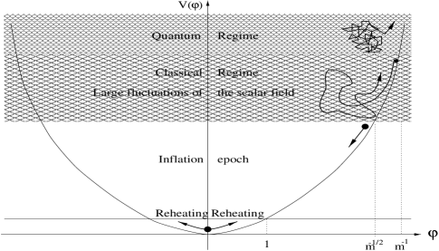
Figure 3.1: Potential energy $V(\varphi)=m^{2}\varphi^{2}/2$. Above the energy scale $1[M_{pl}^{4}]$, quantum gravitational effects are important and the classical interpretation of spacetime brakes down. Above the scale $\varphi\sim m^{-1/2}$, quantum fluctuations of the scalar field are the dominant driving force and can force the field to go both up and down the potential hill. Below this scale, classical evolution is unaffected by quantum fluctuations and the scalar field slowly rolls down the potential. After the field drops below $\varphi\sim 1[M_{pl}]$, inflation ends and the reheating period starts, where oscillations of the scalar field lead to particle creation.

The solution to Eqs. (3.19) and (3.20) for $n=2$ and $k=0$ are straightforward:

$$H\simeq\frac{m}{\sqrt{6}}\varphi$$ (3.21)

and

$$\varphi(t)-\varphi_{i}\simeq-m\sqrt{\frac{2}{3}}(t-t_{i})\quad,$$ (3.22)

where $\varphi_{i}$ is the value of the scalar field at the time $t_{i}$. The Hubble parameter as a function of time is then

$$H(t)\simeq H_{i}-\frac{m^{2}}{3}(t-t_{i})\quad,$$ (3.23)

with $H_{i}=\frac{m}{\sqrt{6}}\varphi_{i}$. The scale factor can be calculated from this expression,

$$a(t)\simeq a_{i}e^{H_{i}(t-t_{i})-\frac{m^{2}}{6}(t-t_{i})^{2}}\quad.$$ (3.24)

It is sometimes useful to use the homogeneous scalar field as a time parameter, and in that case we have the simple expression

$$a(t)\simeq a_{i}e^{\frac{1}{4}(\varphi_{i}^{2}-\varphi^{2})}\quad.$$ (3.25)

Notice that, since $m\ll 1$, the time derivative of the Hubble parameter, $\dot{H}=-m^{2}/3$, is much smaller than $H_{i}\leq m^{1/2}/\sqrt{6}$, that is, it is valid to approximate the Hubble parameter as a constant during inflation. It can also be verified that the kinetic term $\dot{\varphi}^{2}\simeq 2m^{2}/3$ is much smaller than the potential term $m^{2}\varphi^{2}/2$, so that it can be neglected in the expressions for the energy density and pressure. In conclusion, the solutions found are consistent with the approximations, and inflation only makes the solutions more accurate.

During inflation, quantum fluctuations of the scalar field are coupled to the expansion of the universe, which amplifies these fluctuations. After their wavelength crosses the horizon size $H^{-1}$, the fluctuations freeze (their amplitude becomes constant) and quantum corrections cease to be important. These cosmological perturbations from inflation reenter the horizon once inflation is over, and they provide the basis for the inflationary model for structure formation.

We will discuss the generation and evolution of perturbations at greater length in the next section, but for now it suffices to say that the scale at which the fluctuations are generated is approximately constant during inflation. Fluctuations of the size of the Hubble radius have approximately the same amplitude during inflation. After a perturbation becomes larger than the horizon, its amplitude freezes, although its wavelength continues to be redshifted as $\lambda_{ph}\propto a(t)$.

When inflation is over, the Hubble radius increases much faster than $a(t)$, and scales outside the horizon start to cross back into the horizon. Provided the reheating period (see below) is much smaller than the inflationary epoch, the perturbations generated during inflation with same amplitude reenter the Hubble radius $H^{-1}$ after reheating. Since their amplitude has been frozen from the moment they crossed out of the horizon, when they cross back into the horizon their amplitudes are obviously approximately equal. This scale-invariant spectrum of perturbations obtained after the end of inflation is verified by the analysis of the CMB, and constitutes another major success of the inflationary models (but not one exclusive of these models.)

When do inflation end? From Eqs. (3.9) and (3.10) we see that the kinetic term $\dot{\varphi}^{2}/2\simeq 2m^{2}/3$ becomes comparable to $m^{2}\varphi^{2}/2$ when $\varphi=\varphi_{reh}\simeq 1$. At this point the second derivative in the Klein-Gordon equation (3.18), $\ddot{\varphi}$, cannot be neglected anymore. In fact, when the scalar field reaches $\varphi_{reh}$ it accelerates down the potential, since the friction term $3H\dot{\varphi}$ has become much smaller. Another way of seeing this is noting that the natural time scale of the inflaton, $m^{-1}$, becomes equal to the cosmological time scale $H^{-1}$ when $\varphi\simeq 1$, and after the field falls even further, the friction term becomes much smaller, ending the “slow-roll” (see Fig. 3.1.)

In the new regime the scalar field oscillates fastly between two maxima of the potential with very little friction. The Klein-Gordon equation can be approximated by

$$\ddot{\varphi}+m^{2}\varphi\simeq 0\quad,$$ (3.26)

whose solution is straightforward,

$$\varphi(t)\simeq\varphi_{*}\sin{(mt+\theta)}\quad.$$ (3.27)

Notice that energy density and pressure oscillate together with the scalar field, but if we average over a cycle $m^{-1}$ the result is

$$\langle\rho\rangle_{m^{-1}}=\frac{m^{2}\varphi_{*}^{2}}{2}\quad,\quad\langle p\rangle_{m^{-1}}=0\quad.$$ (3.28)

This is the equation of state of pressureless dust, $p=0$, and we know that in that case the continuity equations $\dot{\rho}+3H(\rho+p)=0$ imply that the energy density falls like $a^{-3}$. This time dependence is hidden in $\varphi_{*}$, which in fact decays slowly, while the scale factor falls as a power-law so that the approximation is consistent.

This period of fast oscillations (with period $m^{-1}\gg H^{-1}$) marks the end of cosmological inflation, since the scale factor now grows as a power-law, $a\propto t^{2/3}$. At this point the couplings of the inflaton field to other matter fields becomes also important, and particle production occurs through the mechanism of parametric resonance[24]. This period is known as “reheating”, and is the process by which the empty post-inflationary universe is replenished of the hot particles that we know were present at very early times. Of course, the temperature of the plasma during reheating should not be bigger than the GUT scale, otherwise the problem of monopoles would strike again.

The inflaton field eventually decouples from the other matter sectors, and usually it is assumed that it settles at the minimum of its potential. At the end of reheating virtually all the energy contained in the scalar field at the end of inflation has been converted into ultra-relativistic particles (radiation). Sometimes the inflaton field leaves remnants, and it has been suggested that it could even provide some of the dark or “missing” matter predicted by primordial nucleosynthesis.

3.3 Cosmological perturbations from inflation

One of the main applications of inflationary models is the origin of large-scale structure. Inflation provides a causal mechanism whereby microscopic quantum fluctuations of the scalar field evolve into the classical cosmological perturbations that originated the structure of the universe.

During inflation, the analysis at the end of Chapter 2 shows that the metric perturbations have a time dependence given by Eqs. (2.77) and (2.78),

$$\phi_{k}^{\tiny(HF)}=\dot{\varphi}_{0}\left[A_{k}^{+{\tiny(HF)}}e^{+ik\int dt/a}+A_{k}^{-{\tiny(HF)}}e^{-ik\int dt/a}\right]\quad,$$

when the perturbation is smaller than the horizon, and

$$\phi_{k}^{\tiny(LF)}=A_{k}^{{\tiny(LF)}}\left(1-\frac{H}{a}\int adt\right)\quad,$$

when it is bigger than the horizon.

The factors $A_{k}$ are as yet undetermined, and the classical theory of perturbations does not provide any clue to what their value is. Of course, they are fixed by the initial conditions. When there is no theory available to provide these initial conditions, we can only determine the $A_{k}$’s through the observed inhomogeneities in the present-day universe, and use the theory of cosmological perturbations to deduce what the “seeds” might have looked like at very early times. Modern attempts at explaining large-scale structure such as inflation and topological defects, try to provide physical mechanisms that could generate a spectrum of $A_{k}$ that is consistent with the observed map of the CMBR from a minimal set of parameters and initial conditions. Chaotic Inflation is particularly minimalistic, and necessitates only the self-couplings of the inflaton and its initial value on a homogeneous time slice.

Clearly, the theory about the origins of the seeds are outside the scope of the classical theory of cosmological perturbations. In the inflationary scenario, the mechanism stems from the inherently quantum fluctuations of a scalar field in flat spacetime. In the case of topological defects, the origin of perturbations is a “classical” effect in the sense that the perturbations are created by the motions of macroscopic solitonic objects.

On small wavelengths, fluctuations of the scalar field around a homogeneous background $\varphi_{0}$ can be described by the usual canonical quantum operators acting on a Fock space. When their wavelength crosses the Hubble radius, the fluctuations become squeezed in states with a very high occupancy number, and are thus best described by functions with a statistical distribution. Fluctuations bigger than the horizon during inflation are said to be classical perturbations, in the sense that they follow the classical equations of motion, $\delta G_{\mu\nu}=\delta T_{\mu\nu}$, without quantum corrections.

Fluctuations of the homogeneous scalar field inside the horizon can be treated by quantum field theory. Outside the horizon the expectation value of the field excitations is very high, and can be replaced by a sum over momentum modes of classical fields with amplitudes obeying a Gaussian statistical distribution. The spatial average $\langle\delta f\rangle$ of linear perturbations yield zero identically, just as happens with the expectation value of a linear quantum fluctuation ($\langle 0|\delta f^{+}a^{+}+\delta f^{-}a^{-}|0\rangle=0$ at all times). The notion of spatial average here is defined on the biggest possible scale, that is, on the scale of the physical radius of the entire inflating bubble, $H^{-1}(t_{i})a(t)/a(t_{i})\gg H^{-1}(t)$, where $t_{i}$ is the time when inflation started in that bubble. Of course, fluctuations around the homogeneous value are by definition zero on this largest scale, although they might be nonzero on smaller domains inside the initial bubble.

The two-point functions of fluctuations, as opposed to linear functions of the perturbations, do not vanish in general, $\langle 0|\delta\hat{f}_{k}\delta\hat{f}_{k^{\prime}}|0\rangle\propto\delta_{k^{\prime}k}$. Knowledge of the correlation functions of field operators at the horizon scale ($|k|\sim H$) gives the amplitudes of modes $|\delta f_{k}|^{2}$ with a classical interpretation and Gaussian statistics.

The reasoning used below is as follows: we first determine the amplitude of the modes of the perturbations when they cross outside the horizon. That fixes the amplitudes of all modes created during inflation that are of cosmological interest. We then just follow the classical evolution of the modes to obtain the spectrum of the perturbations, both during inflation when their wavelength is exponentially bigger than the horizon $H^{-1}$, and after inflation ends when they start to reenter the horizon.

We start by presenting a non-rigorous derivation[5] of the “spectrum” $\phi_{k}$, based on the Hawking temperature associated with a de Sitter spacetime[25]. Quantum fluctuations of the scalar field on scales of order the Hubble radius $H^{-1}$ should have an amplitude proportional to the Hawking temperature of the thermal fluctuations of de Sitter. Their root mean square value on a sphere with a radius of the size of the Hubble horizon is then

$$|\delta\varphi_{H}|\sim T_{H}=\frac{H}{2\pi}\quad.$$ (3.29)

Since $\varphi(t)\gg 1[M_{pl}]$ and $H\sim m\varphi_{0}(t)$ during inflation, these perturbations are small, as expected: $\delta\varphi/\varphi_{0}\ll 1$. The energy density of the universe, during inflation, is dominated by the potential energy $V(\varphi)$, and thus fluctuations with scales close to the Hubble horizon should also be proportional to the fluctuations of the scalar field, $\delta\rho_{H}/\rho\sim\delta V/V$. Using the model with $V=m^{2}\varphi^{2}/2$ and Eq. (3.29), as well as the identity[13] $\left.\frac{\delta\rho}{\rho}\right|_{k(t)}=-2\phi|_{k(t)}$ valid when the perturbation crosses the horizon, $k(t)=H$, we get that, during inflation, the amplitude of the modes for the scalar perturbation $\phi_{H}$ is (up to some numerical coefficients),

$$|\phi_{H}|\simeq m\quad.$$ (3.30)

This amplitude corresponds to a perturbation on the scale of the Hubble radius, and real perturbations are expected to be positive or negative, that is, the fluctuations either raise or lower the energy density inside the horizon.

We are primarily interested in the spectrum of the momentum modes, so we need to perform a Fourier transformation starting from the fluctuations $\phi_{H}(r)$. This quantity reflects net perturbations inside a sphere of radius $r$, and its value can assume both negative and positive values. The best we can do then is to evaluate the square of this quantity on spheres of radius $r$. The integration over volume inside the sphere introduces a factor of $r^{3}\sim k^{-3}(r)$, so we find the result

$$\phi_{k(r)}^{2}\simeq k^{-3}(r)\left|\phi_{H}\right|_{r}^{2}\quad\rightarrow\quad|\phi_{k(r)}|\simeq k^{-3/2}(r)\left|\phi_{H}\right|_{r}\quad.$$ (3.31)

$\left|\phi\right|_{k(r)}^{2}$ is usually referred to as the power spectrum of the field $\phi$ at the scale k(r). We finally find that, for quantum fluctuations with size comparable to the Hubble radius, $k\sim H$,

$$|\phi|_{k}\simeq k^{-3/2}m\quad.$$ (3.32)

Due to the special time-translation invariance properties of de Sitter spacetime, we can generalize this result to other scales. As soon as the physical wavelength of a fluctuation becomes bigger than the horizon, the time dependence of its amplitude $\phi_{k}$ is given by the classical equations of motion and, as a consequence, its amplitude freezes [actually it evolves very slowly with time, $\dot{\phi}_{k}/\phi_{k}\ll H$, see Eq. (2.78)]. What that means is that we can assume that the amplitudes (3.30) carries on for a long time after the perturbation leaves the horizon, and, as long as inflation goes on, this amplitude is approximately constant. Therefore, during inflation and for modes with wavelengths bigger than the horizon, the spectrum is given by (3.30), where the $k$’s correspond to scales bigger than the horizon, $k>H$.

The argument above relied on a separation between the classical and the quantum regime that was criticized for being artificial. The full quantum treatment is slightly more complicated, but the end result, Eq. (3.32) during inflation, is essentially the same.

We now proceed to the full quantum treatment of the creation of perturbations[13]. Our aim is to quantize, using the canonical scheme, the coupled scalar and metric perturbations, and calculate their two-point correlation functions $\langle\delta\hat{f}^{2}\rangle$. In order to use the variational principles (find the canonically conjugated momenta and the Hamiltonian), the action must be determined to second order in the perturbations. We start from the fundamental action

$$S=\int\sqrt{-g}d^{4}x\left\{-\frac{1}{2}R+{\cal L}_{m}\right\}\quad,$$ (3.33)

where $R$ is the Ricci scalar curvature and ${\cal L}_{m}$ is the Lagrange density function for the matter sector. We are interested in a scalar field, for which

$${\cal L}_{\varphi}=\frac{1}{2}D^{\mu}\varphi D_{\mu}\varphi-V(\varphi)\quad.$$ (3.34)

We should now expand the action (3.33) to second order in the scalar perturbations $\phi$ and $\delta\varphi$, around the flat FRW background with $a(t)$ and $\varphi_{0}(t)$. The $0^{th}$-order term gives the equations for the backgrounds, while the $1^{st}$-order term is identically zero (its variation $\delta S$ is proportional to the background equations of motion).

It turns out that, due to the constraint (2.65), there is only one dynamical variable expressing scalar perturbations, the gauge-invariant potential ${{\vartheta}}$. We shall find explicit solutions for the modes ${\vartheta}_{k}$, then relate those to the modes $\delta\varphi_{k}$ and $\phi_{k}$. Finally, we give explicit expressions for the spectra of the scalar perturbations.

The action in terms of ${\vartheta}$ is most easily expressed in conformal time, and we simply state the result here (for a detailed discussion, see Ref. [13]):

$$\delta^{2}S=\frac{1}{2}\int d^{4}x\left\{{\vartheta}^{\prime 2}-(\nabla{\vartheta})^{2}+\frac{z^{\prime\prime}}{z}{\vartheta}^{2}\right\}\quad,$$ (3.35)

where we have discarded several total derivatives that do not affect the quantization procedure or the classical evolution. The potential ${\vartheta}$ has dimensions of mass, and is defined as

$${\vartheta}(\eta,\vec{x}) = a\delta\varphi(\eta,\vec{x})+z\phi(\eta\vec{x})\quad,$$ (3.36)

$$z(\eta) = a{\varphi_{0}}^{\prime}/{\cal H}\quad,$$

where ${\cal H}=a^{\prime}/a$. The action (3.35) describes a scalar field ${\vartheta}$ with a time-dependent mass $M^{2}=-z^{\prime\prime}/z$, in analogy with the equation of motion (2.70) for the perturbation $u$ defined in Section 2.6 . This mass is, as before, a function of the background quantities $\varphi_{0}(\eta)$ and ${\cal H}$. When the scalar field is not rolling down the potential, ${\varphi_{0}}^{\prime}=0=z$, the perturbations are not amplified and as a consequence there is no creation of particles. The quantization procedure used here is also analogous to the quantization of scalar fields in Minkowski space-time in the presence of external fields.

The second step in canonical quantization is to determine the canonical momenta associated with ${\vartheta}$, and impose the commutation relations between the field operators and the canonically conjugated momenta. The momenta are defined with the help of (3.35) as

$$\pi(\eta,\vec{x})=\frac{\partial{\cal L}^{(2)}}{\partial{\vartheta}^{\prime}}={\vartheta}^{\prime}\quad.$$ (3.37)

In the quantum theory, fields and momenta ${\vartheta}$ and $\pi$ are raised to the category of Heisenberg operators $\hat{\vartheta}$ and $\hat{\pi}$, and we impose the canonical same-time commutation relations

$$[\hat{\vartheta}(\eta,\vec{x}),\hat{\vartheta}(\eta,\vec{x}^{\prime})]=[\hat{\pi}(\eta,\vec{x}),\hat{\pi}(\eta,\vec{x}^{\prime})]=0$$ (3.38)

and

$$[\hat{\vartheta}(\eta,\vec{x}),\hat{\pi}(\eta,\vec{x}^{\prime})]=i\delta(\vec{x}-\vec{x}^{\prime})\quad.$$ (3.39)

The dynamics of the field operators is given by the hamiltonian equations of motion

$$i\hat{\vartheta}^{\prime}=[\hat{\vartheta},\hat{H}]\quad,\quad i\hat{\pi}^{\prime}=[\hat{\pi},\hat{H}]\quad,$$ (3.40)

where the Hamiltonian can be easily reconstructed from the second-order action $\delta^{2}S$,

$$\hat{H}=\int d^{3}x({\vartheta}^{\prime}\pi-{\cal L})=\frac{1}{2}\int d^{3}x\left\{\pi^{2}+(\nabla{\vartheta})^{2}-\frac{z^{\prime\prime}}{z}{\vartheta}^{2}\right\}\quad.$$ (3.41)

The equation of motion for $\hat{\vartheta}$ can be obtained from the hamiltonian system (3.40), or equivalently by varying the action $\delta^{2}S$ with respect to the field ${\vartheta}$:

$$\hat{\vartheta}^{\prime\prime}-\nabla^{2}\hat{\vartheta}-\frac{z^{\prime\prime}}{z}\hat{\vartheta}=0\quad.$$ (3.42)

The best way to solve this equation is, clearly, to expand the field in plane waves (generalized spherical harmonics in the case of open and closed spaces):

$${\vartheta}(\eta,\vec{x})=\frac{1}{\sqrt{2}}\int\frac{d^{3}k}{(2\pi)^{3}/2}\left[{\vartheta}_{k}^{\ast}e^{i\vec{k}\vec{x}}a^{-}_{k}+{\vartheta}_{k}e^{-i\vec{k}\vec{x}}a^{+}_{k}\right]\quad,$$ (3.43)

where the operators $\hat{a}$ will be interpreted as raising and lowering (creation and annihilation) operators acting on the vacuum $|0\rangle$ of the Fock space representation (we use the Heisenberg representation). All time dependence is contained in the functions ${\vartheta}_{k}(\eta)$, which now satisfy the equations

$${{\vartheta}_{k}}^{\prime\prime}+(k^{2}-{z^{\prime\prime}}/{z}){\vartheta}_{k}=0\quad.$$ (3.44)

In terms of the creation and annihilation operators, the commutation relations are the ones for a simple harmonic oscillator,

$$[a_{k}^{-},a_{k^{\prime}}^{-}]=[a_{k}^{+},a_{k^{\prime}}^{+}]=0\quad,\quad[a_{k}^{-},a_{k^{\prime}}^{+}]=\delta(\vec{k}-\vec{k^{\prime}})\quad.$$ (3.45)

The mode functions ${\vartheta}_{k}(\eta)$ must obey the following normalization conditions so that the last commutation relation is equivalent to $[{\vartheta}(x),\pi(x^{\prime})]=i\delta(x-x^{\prime})$:

$${\vartheta}_{k}^{\prime}{\vartheta}_{k}^{\ast}-{{\vartheta}_{k}^{\ast}}^{\prime}{\vartheta}_{k}=2i\quad.$$ (3.46)

Usually, modes associated with the annihilation operator $\hat{a}_{k}$ have a positive frequency $w^{2}(k)=k^{2}+M^{2}$, while the modes corresponding to $\hat{a}^{\dagger}$ have negative frequency. In our case the mass term $M^{2}=-z^{\prime\prime}/z$ is time-dependent, leading to a mixing between the positive- and negative-frequency modes associated with $a^{-}_{k}$ and $a^{+}_{k}$. Hence, even if we define a vacuum state for the Fock representation at some initial conformal time $|0,\eta_{1}\rangle$, this vacuum will appear to have a non-vanishing particle content at a later time, $a^{-}_{k}(\eta_{2}>\eta_{1})|0,\eta_{1}\rangle\neq 0$. Mathematically, it is possible to define eigenfunctions $\psi_{k}(\eta_{1})$ of the creation and annihilation operators at time $\eta_{1}$, but these cannot be expressed in terms of eigenfunctions at a later time $\eta_{2}$, $\psi_{k}(\eta_{2})$. The number operator at time $\eta_{1}$, $N_{k}^{1}=a_{k}^{+}(\eta_{1})a_{k}^{-}(\eta_{1})$, vanishes for the vacuum $|0,\eta_{1}\rangle$, but is not zero if the operator is evaluated at a later time,

$$\langle N_{k}^{2}\rangle_{\eta_{1}}=\langle 0,\eta_{1}|N_{k}(\eta_{2})|0,\eta_{1}\rangle\neq 0\quad.$$ (3.47)

Conversely, it is equivalent to say that the creation and annihilation operators at different times mix with each other. With that perspective, it makes no sense to define a unique set of eigenfunctions that are annihilated by all operators $a_{k}^{-}(t)$. The linear transformations that relates creation and annihilation operators at different times are called Bogoliubov transformations:

$$\left(\begin{array}[]{c}a_{k}^{-}(\eta_{2})\\ a_{k}^{+}(\eta_{2})\end{array}\right)=\left(\begin{array}[]{cc}\alpha_{k}(\eta_{1},\eta_{2})&\beta_{k}^{\ast}(\eta_{1},\eta_{2})\\ \beta_{k}(\eta_{1},\eta_{2})&\alpha_{k}^{\ast}(\eta_{1},\eta_{2})\end{array}\right)\left(\begin{array}[]{c}a_{k}^{-}(\eta_{1})\\ a_{k}^{+}(\eta_{1})\end{array}\right)\quad,$$ (3.48)

where unitarity implies that $|\alpha_{k}|^{2}-|\beta_{k}|^{2}=1$.

If we define the number operator at the time $\eta_{2}$ in terms of the vacuum at $\eta_{2}$, it is clear that, at an earlier time $\eta_{1}$, the occupation number is given by

$$\langle N_{k}^{2}\rangle_{\eta_{1}} = \langle 0,\eta_{1}|a_{k}^{+}(\eta_{2})a_{k}^{-}(\eta_{2})|0,\eta_{1}\rangle$$

$$= \langle 0,\eta_{1}|a_{k}^{-}(\eta_{1})\beta_{k}(\eta_{1},\eta_{2})\beta_{k}^{\ast}(\eta_{1},\eta_{2})a_{k}^{+}(\eta_{1})|0,\eta_{1}\rangle=|\beta_{k}(\eta_{1},\eta_{2})|^{2}\quad,$$

and conversely, if we define the vacuum at $\eta_{2}$, the number operator defined in terms of the vacuum at $\eta_{1}$ has the expectation value

$$\langle N_{k}^{1}\rangle_{\eta_{2}}=\langle 0,\eta_{2}|a_{k}^{+}(\eta_{1})a_{k}^{-}(\eta_{1})|0,\eta_{2}\rangle=|\beta_{k}(\eta_{2},\eta_{1})|^{2}\quad.$$ (3.50)

The “forward” ($\eta_{1}\rightarrow\eta_{2}$) and “backward” ($\eta_{1}\leftarrow\eta_{2}$) Bogoliubov coefficients can be related by inverting the matrix (3.48) and taking into account the unitarity constraint,

$$\alpha_{k}(\eta_{2},\eta_{1})=\alpha^{\ast}(\eta_{1},\eta_{2})\quad,\quad\beta_{k}(\eta_{2},\eta_{1})=-\beta(\eta_{1},\eta_{2})\quad,$$ (3.51)

therefore it is a consequence of unitarity that $\langle N_{k}^{1}\rangle_{\eta_{2}}=\langle N_{k}^{2}\rangle_{\eta_{1}}$.

To summarize, an observer at $\eta_{2}$ will measure a nonvanishing number of particles $N^{2}_{k}(\eta_{1})$ in the “vacuum” state $|0,\eta_{1}\rangle$ as long as the Bogoliubov transformations are not trivial, i.e., as long as $\beta_{k}\neq 0$. This “particle production” from an initial vacuum state is a consequence of the time-dependent background external fields, and is the mechanism responsible for the origin of cosmological perturbations in inflationary models.

The ambiguity in chosing a vacuum is related to the freedom in choosing the precise initial conditions for the mode functions ${\vartheta}_{k}$ and ${\vartheta}_{k}^{\prime}$ at some initial time. Since the equations of motion that determine the ${\vartheta}_{k}$’s is second-order in time, there are two integration constants that must be fixed. The normalization constraints (3.46) reduce the number to one free parameter, which is essentially the choice of an initial time $\eta_{0}$ such that the vacuum $|0,\eta_{0}\rangle$ is empty at $\eta_{0}$.

During the inflating period, high frequency modes are redshifted by the expansion of the universe, and eventually become low frequency. We will define the vacuum states in the limit $k\rightarrow\infty$, when the perturbations are well inside the horizon and we can consider the background to be approximated by flat Minkowski, therefore the ambiguity in the definition of a particle that occurs for long wavelength modes in curved spacetimes is absent[13]. The equations of motion (3.44) and the normalization conditions (3.46) imply that the mode functions are

$${\vartheta}_{k}(\eta_{i})\simeq M(k\eta_{i})k^{-1/2}e^{+ik\eta_{i}}\quad,\quad{\vartheta}_{k}^{\prime}(\eta_{i})\simeq iN(k\eta_{i})k^{1/2}e^{+ik\eta_{i}}\quad\quad(k\eta_{i}\gg 1)\quad,$$ (3.52)

where $|M(k\eta_{i})|\rightarrow 1$ and $|N(k\eta_{i})|\rightarrow 1$ when $k\eta_{i}\gg 1$ and the normalization condition is

$$MN^{\ast}+M^{\ast}N=2\quad.$$ (3.53)

The time $\eta_{i}$ can be chosen to be the time when the inflationary epoch begins, so that the vacuum is defined with respect to this initial moment. If there are particles or inhomogeneities present at that moment such that vacuum would not be the appropriate definition, this “initial time” can be chosen a few e-folds later, when the expansion of the universe will have diluted the initial deformities.

The choice of initial time is akin to the choice of initial conditions on a big enough patch of the universe. Since the observed universe originated inside the Hubble radius at $N\simeq 50$ e-folds before the end of inflation, we could chose this initial time as being any moment from the beginning of inflation up to the time $\eta_{60}$ when there were $60$ e-folds left to the end of inflation. Although the choice of initial vacuum in this time interval does not alter the results of calculations of the CMBR, it will play a significant role when we discuss the global features of the chaotic scenario, that is, features of the spacetime on scales of the particle horizon $H^{-1}(t_{i})a(t_{0})/a(t_{i})$ and larger ($t_{0}$ is the time now and $t_{i}$, as before, is the time when inflation started.) Notice that if inflation occurred for more than $60$ $e$-folds, the particle horizon could be many orders of magnitude bigger than the presently observable universe.

We now wish to go back to the scalar perturbations $\phi$ and $\delta\varphi$. First, remember that the two are related by the constraint (2.65),

$$\phi^{\prime}+{\cal H}\phi=\frac{1}{2}\varphi_{0}^{\prime}\delta\varphi\quad,$$

so that all we have to do is relate ${\vartheta}$ to $\phi$. From the definition of ${\vartheta}$, (3.36), and Eq. (2.66), it is straightforward to obtain, after some juggling with algebra, that

$$\phi_{k}(\eta)=-\frac{1}{k^{2}}\frac{\varphi_{0}^{\prime 2}}{{\cal H}}\left(\frac{{\vartheta}_{k}}{z}\right)^{\prime}\quad$$ (3.54)

where, as before, $z=a\varphi_{0}^{\prime}/{\cal H}$.

The reason why we used the potential ${\vartheta}$ instead of the variable $\phi$ in the quantization procedure is that the action in terms of $\phi$ is much more complicated, and thus the quantization much more involved when written in terms of that variable.

The equation obeyed by $\phi_{k}$ have been derived before, see Eq. (2.70),

$$u_{k}^{\prime\prime}+k^{2}u_{k}-\frac{(1/z)^{\prime\prime}}{1/z}u_{k}=0\quad,$$ (3.55)

where the variable $u_{k}=a\phi_{k}/\varphi_{0}^{\prime}$, introduced in Eq. (2.71), is obviously related to ${\vartheta}_{k}$ by

$$u_{k}=-\frac{1}{k^{2}}\frac{z}{2}\left(\frac{{\vartheta}_{k}}{z}\right)^{\prime}\quad.$$ (3.56)

We will use now explicit solutions to $u_{k}$ in the short and long wavelength limits, and subject them to the constraints (3.52) and (3.53), found through the quantization of the ${\vartheta}$-modes. First, in the short wavelength limit of Eqs. (3.55), $k^{2}\gg(1/z)^{\prime\prime}/(1/z)$, there are clearly oscillating solutions with frequency $k$. We impose on these solutions the constraints found upon quantization, (3.52), which, using the relations above, are

$$u_{k}(\eta_{i}) = -\frac{1}{2}\left[\frac{i}{k^{3/2}}N(k\eta_{i})-\frac{z^{\prime}(\eta_{i})}{z(\eta_{i})}\frac{1}{k^{5/2}}M(k\eta_{i})\right]\quad,$$ (3.57)

$$u_{k}^{\prime}(\eta_{i}) = -\frac{1}{2}\left[\frac{1}{k^{3/2}}M(k\eta_{i})+3\frac{z^{\prime}(\eta_{i})}{z(\eta_{i})}\left(\frac{i}{k^{3/2}}N(k\eta_{i})-\frac{z^{\prime}(\eta_{i})}{z(\eta_{i})}\frac{1}{k^{5/2}}M(k\eta_{i})\right)\right]\quad.$$

The solutions in the high frequency, small wavelength limit are then written as

$$u_{k}(\eta)=u_{k}(\eta_{i})\cos{[k(\eta-\eta_{i})]}+\frac{u_{k}^{\prime}(\eta_{i})}{k}\sin{[k(\eta-\eta_{i})]}\quad.$$ (3.59)

The low frequency, long wavelength solutions [when $k^{2}\ll(1/z)^{\prime\prime}/(1/z)$ ] are

$$u_{k}=A_{k}\frac{1}{z}\int d\eta z^{2}\quad,$$

but we can use the background equations inside the integral, integrate by parts and the final result is

$$u_{k}(\eta)=A_{k}\frac{1}{\varphi_{0}^{\prime}}\left(\frac{1}{a}\int d\eta a^{2}\right)^{\prime}\quad.$$ (3.60)

So far the constants $A_{k}$ (which, as we discussed before, determine the spectrum of the long wavelength perturbations) are undetermined. But the spectrum $u_{k}(\eta_{i})$ for small wavelengths has been fixed by quantization. Therefore, what we have to do to determine the $A_{k}$’s is follow a short wavelength mode with physical wavelength $\lambda_{ph}=2\pi a/k$ until it reaches the limiting wavelength $2\pi ak^{-1}_{\eta_{{}_{\cal H}}}\sim\sqrt{(1/z)/(1/z)^{\prime\prime}}$, and then use the junction conditions to fix the amplitude of that mode for all later times.

A rigorous treatment would forcibly involve the approximate solutions when $k^{2}\sim(1/z)^{\prime\prime}/(1/z)$, which are very difficult to obtain. There is a much simpler way, though, which involves taking into account the relation between the ${\vartheta}_{k}$ and $u_{k}$ given in Eq. (3.56). We know that for the ${\vartheta}_{k}$ modes the scale above which the fluctuations are high frequency is $k_{\vartheta}^{2}=z^{\prime\prime}/z$. For the $u_{k}$ modes, though, that scale is $k_{u}^{2}=(1/z)^{\prime\prime}/(1/z)$. Therefore, if these scales overlap over a wide enough band, both the oscillatory solutions (3.59) and the large-wavelength solutions (3.60) must be good approximations to the exact solution. During an inflationary period, this interval is indeed large, in fact

$$z\left(\frac{1}{z}\right)^{\prime\prime}\simeq m^{2}a^{2}(\eta)\quad\ll\quad\frac{z^{\prime\prime}}{z}\simeq{\cal H}^{2}(\eta)\simeq\frac{m^{2}}{6}\varphi_{0}^{2}(\eta)a^{2}(\eta)\quad,$$

since $\varphi_{0}\gg 1$ during inflation. Therefore, for scales such that $ma(\eta)<k<{\cal H}(\eta)$, both solutions are approximately valid. We can then express the approximate solutions in this interval as

$$u_{k}(\eta)=\frac{u_{k}(\eta_{i})\cos{(k\eta_{i})}-[u_{k}^{\prime}(\eta_{i})/k]\sin{(k\eta_{i})}}{\{(1/\varphi_{0}^{\prime})[(1/a)\int d\eta a^{2}]^{\prime}\}_{\eta_{\cal H}(k)}}\frac{1}{\varphi_{0}^{\prime}}\left(\frac{1}{a}\int d\eta a^{2}\right)^{\prime}\quad,$$ (3.61)

where the junction time $\eta_{\cal H}(k)$ represents the time when the scale $k={\cal H}(\eta_{\cal H}(k))$ crosses the Hubble radius, that is, when the physical wavelength of the mode $k$, $\lambda_{ph}=2\pi a(\eta)/k$, becomes bigger than the horizon $H^{-1}=a{\cal H}{-1}$.

Therefore, formulas (3.61) and (3.59) are, respectively, valid for long wavelength and short wavelength perturbations in an inflationary universe. We will use these formulas to calculate the amplitude in each mode of the field $\phi_{k}$, for $k$’s representing both perturbations bigger and smaller than the horizon. As noted after Eq. (3.55), the modes $\phi_{k}$ can be expressed in terms of the modes $u_{k}$ by

$$\phi_{k}(\eta)=\frac{\varphi_{0}^{\prime}}{a}u_{k}(\eta)\quad.$$ (3.62)

For the simple case when the inflaton potential is $V=m^{2}\varphi^{2}/2$, the expressions for long and short waves simplify substantially, and after we take into account the approximate solutions for the scale factor in (3.25), approximation (3.21) and the useful indentity ${\cal H}\simeq-2\varphi_{0}^{\prime}\varphi_{0}$ the result is

$$|\phi_{k}|(t)=k^{-3/2}\frac{m}{2\sqrt{6}\pi}\times\left\{\begin{array}[]{ll}1\\ \left[1-\frac{4}{\varphi_{0}^{2}(t)-\varphi_{0}^{2}(t_{r})}\log{\left(\frac{k}{H(t)a(t)}\right)}\right]\,,\end{array}\right.$$ (3.63)

with $k>H(t)a(t)$ in the former case and $\quad H_{i}a(t_{i})<k<H(t)a(t)$ in the latter. In this expression, $t_{i}$ is the time when inflation started, and $t_{r}$ is the time when it ends. To the reader concerned with units, we note that had we retained units in the expression above, we would get $m/M_{pl}$ (or $\sqrt{G}m$) instead of $m$. We also notice that we have retrieved the result of Eq. (3.32), with a logarithmic correction that comes from the fact that the Hubble parameter is only approximately constant during inflation, such that the Hawking temperature at the beginning of inflation is bigger than that at the end.

We can also calculate the amplitude of perturbations after inflation is over. Assuming that the universe behaves essentially as if it was dominated by radiation, the scale factor has the time dependence $a\propto t^{1/2}$ (this is a good approximation because during the brief period of reheating, $a\propto t^{2/3}$). The result is very simple,

$$\phi_{k}(t>t_{r})\simeq k^{-3/2}m\log{(\frac{\lambda_{ph}}{\lambda_{\gamma}})}\quad,$$ (3.64)

where $\lambda_{ph}=2\pi a(t)/k$ is the physical wavelength of the perturbation with comoving wavenumber $k$, and $\lambda_{\gamma}$ is the characteristic wavelength of the cosmic background radiation.

In observational cosmology the object of interest is the power spectrum, which, as mentioned at the beginning of this section, is defined as the adimensional measure of a classical fluctuation moded out by a volume factor, e.g.,

$$\left|\delta^{\phi}_{k}\right|\equiv k^{3/2}\left|\phi_{k}\right|\quad$$ (3.65)

and

$$\left|\delta^{\delta\varphi}_{k}\right|\equiv k^{3/2}\left|\frac{\delta\varphi_{k}}{\varphi_{0}}\right|\quad.$$ (3.66)

From Eqs. (3.63) and (3.64) we see that the power spectrum of the scalar perturbations created during inflation is nearly scale invariant, with only logarithmic corrections that are not very important on scales that are relevant cosmologically. The power spectrum is also proportional to the square root of the self-coupling of the scalar field ($\sqrt{m^{2}}$ in our case of a massive inflaton). The fluctuations in the temperature seen in the CMBR are roughly proportional to the spectrum calculated above, and the amplitude measured is about $\delta T/T\sim 5\times 10^{-6}$. This implies that the mass of the inflaton has to be very small, $m\sim 10^{-6}[M_{pl}]$, so that the perturbations created by inflation have the correct amplitude. That the mass of the inflaton happens to be so small is referred to as the “fine-tuning problem”.

Summarizing, we saw that inflation provides a causal mechanism that generates perturbations with near identical amplitudes on cosmological scales. The power spectrum of perturbations is nearly scale-invariant, and is proportional to the mass of the inflaton. These perturbations are generated continuously during inflation, inside the causal Hubble horizon. They leave during inflation (their physical wavelengths become bigger than the horizon) and reenter later, after inflation ends.

3.4 Global structure of Chaotic Inflation

We have mentioned in Section 3.2 that, above a certain scale, large quantum fluctuations of the scalar field might give rise to a process that generates new inflating bubbles . We will see later that the back reaction of scalar perturbations created during inflation is important on scales where the process of self-reproduction is active. In this section we explain how the chaotic inflationary model can regenerate itself, and investigate some features of the universe on very large scales[5].

It was shown in the last section that small wavelength quantum fluctuations originated inside the Hubble horizon have their amplitude magnified, and their wavelength redshifted, as inflation proceeds. If perturbations have a small amplitude, they don’t have a noticeable effect on the evolution of bubbles. On the other hand, if a perturbation in the energy density inside an initial bubble is so large that after it leaves the horizon the background energy density in “new” bubbles is affected, then the perturbations have to be accounted for in the dynamics of these bubbles[26].

We will show below that above a certain energy scale (the so-called “self-reproducing scale”), quantum fluctuations of the scalar field are so large that they are dominant in the dynamics of the bubbles, and actually drive the scalar field up its potential hill in most regions of the universe[27]. Since the expansion rate is proportional to the potential energy of the scalar field, regions in which the scalar field is higher up its potential expand faster, and as a result these bubbles dominate the ultra-large scale structure of the universe. A bubble in which the scalar field happened to fall below the self-reproducing scale (called also a “mini-universe”) evolves classically, in the sense that the classical equation of motion for the scalar field (2.15) is obeyed, without quantum corrections. The expansion rates of these classical mini-universes are much slower than elsewhere, therefore they occupy an ever decreasing volume fraction in the universe.

In bubbles where the energy density is above the self-reproducing scale, quantum fluctuations drive the scalar field both up and down the potential. As a result, after a few e-folds an initially homogeneous bubble would turn into a rather inhomogeneous collection of bubbles, some with higher, some with lower energy density (see Fig. 3.2). From a homogeneous bubble, after a few e-folds we would get many different bubbles with different energy densities, expansion rates etc. In particular, the process could drive the energy density in some regions to such high values that the symmetries of the fundamental Grand Unifyed Theory would be restored. If a domain happens to cool down and come out of this symmetry-restored region to become a FRW universe, the physical properties of this “baby universe” could be radically different from ours, since its GUT vacuum is not necessarily the same as ours. Hence the names “self-reproduction” and ”mini-universes”: according to the chaotic scenario, there is a continuous creation of inflating bubbles, each of which might have completely different physics.

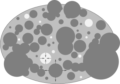
Figure 3.2: A region of constant comoving volume with an average value of the scalar field $\bar{\varphi}>\varphi_{sr}$ (“initially homogeneous bubble”). Dark bubbles correspond to domains where the scalar field fluctuated to a value bigger than $\bar{\varphi}$, and in the light bubbles it fluctuated down to $\varphi<\varphi_{sr}$. The dark bubbles occupy an exponentially high comoving volume of the initial bubble, since their Hubble parameter is bigger than the Hubble parameter of the initial bubble.

In all fairness, the global structure of the chaotic scenario bears no immediate concerns for astronomers preoccupied with the observable universe, since all of it would have come from an entirely classical region some $60$ $e$-folds before reheating. However, it is crucial when we consider, for example, the nature of the Big Bang singularity, the initial conditions for the universe and its topology, and as a means to justify the anthropic principle in inflationary cosmology.

A rigorous analysis of the global structure involves the diffusion equation for the probability distribution of the value of the scalar field, $P(\varphi,t)$. The final result, though, is the same as the one obtained by a much simpler argument explained below[5].

A classical description of spacetime is only possible when the energy density of the universe has fallen below $\rho\sim V(\varphi)\sim 1[M_{pl}^{4}]$. The value of the scalar field, in the massive case, is by assumption smaller than $\varphi<\varphi_{pl}=m^{-1}$, with the mass constrained by the observed CMB anisotropies to be $m\sim<10^{-6}$. A microscopic domain of the size of a Hubble radius $H_{pl}^{-}1\sim l_{pl}=10^{-44}$ cm would have inflated to a radius today of about

$$R(t_{0})\sim l_{pl}e^{-\frac{1}{4}[\varphi^{2}(t_{0})-\varphi_{pl}^{2}]}\sim e^{10^{10}}{\rm cm}\quad,$$ (3.67)

quite a few orders of magnitude bigger than the observable universe today. Notice that the estimate above is actually a lower bound, since we know that quantum fluctuations should make most regions inside the initial planck-size bubble inflate for much longer than that.

The generation of long wavelength perturbations is completely analogous to the mechanism described in the previous chapter: quantum perturbations of the scalar field are redshifted, while their amplitude is approximately frozen once they become larger than the horizon. The difference is the amplitude of the quantum fluctuations in a region of the universe in which the scalar field is above the self-reproducing scale. As we have noted before, quantum fluctuations during inflation have a power spectrum given by

$$|\Delta^{Q}\varphi|\sim\frac{H}{2\pi}\quad,$$ (3.68)

which can be interpreted as meaning that the scalar field takes a step of size $H/2\pi$ every time lapse $\Delta t=H^{-1}$.

At the same time, the approximate equation of motion during inflation, Eq. (3.19), implies that after the same time lapse $H^{-1}$ the change in the scalar field from the force $V_{,\varphi}$ will be

$$\Delta^{Cl}\varphi\simeq\frac{V_{,\varphi}}{V}H^{-1}\simeq\frac{2}{\varphi}\quad.$$ (3.69)

By comparing the two values we see that if we require that quantum fluctuations be unimportant, then

$$\varphi\ll\varphi_{sr}=m^{-1/2}\quad,$$ (3.70)

and the converse if the classical motion of the scalar field is negligible when compared to the quantum fluctuations. Notice that even though the quantum fluctuations are important in this limit, we still have $|\delta\varphi/\varphi|\ll 1$ so that the linear perturbative approach is still valid.

The behavior of a domain with $\varphi<\varphi_{sr}$ is very simple, and is given by the familiar picture of a scalar field rolling down the hill of the potential. Regions in which $\varphi>\varphi_{sr}$ are much more interesting, since they can show a multitude of distinct behaviors, including mini-universes with radically different physical properties. The continuous creation of inflating bubbles from other inflating bubbles means that spacetime has a fractal structure, maybe even a self-similar one. Given the virtually infinite variety of mini-universes that can be created, the chaotic scenario implies that some universes must be capable of supporting life.

The main result from this section is Eq. (3.70): above the self-reproducing scale, quantum fluctuations dominate the evolution of the scalar field. In a mini-universe like ours, the value of the scalar field at the beginning of inflation was $\varphi_{sr}=m^{-1/2}$, and it rolled down from there. The total size of our mini-universe is then roughly $L_{0}\sim 10^{10^{5}}$ cm, still a number for which units are quite meaningless.

The main point of this monograph is to show that the influence of the quantum creation of perturbations is not restricted to the effect to linear order caused by fluctuations in the self-reproducing epoch. In the next chapter we discuss how cosmological perturbations for which the linear effect is negligible can still have a decisive effect on the dynamics of the background.

Chapter 4 The Effective Energy-momentum Tensor

Gravitational waves curve the space in which they propagate. But how can the gravitational field be at the same time the cause and effect of the gravitational field? What is the difference between the gravitons that make up a gravity wave and the gravitons that constitute a background metric in which the gravity waves propagate? How do they interact?

Due to the nonlinearities of Einstein’s equations, the notions of gravitational fields and sources are not as markedly distinct as in other field theories like electromagnetism. Indeed, if gravity can be described by anything that looks like a quantum field theory, then in some classical limit of this theory there is a spin-2 massless particle, the graviton. The propagation of gravitons in flat spacetime can be described in terms of transversal plane wave solutions to the classical (usually Einstein’s) theory. These waves, parametrized by a wavenumber $\vec{k}$, clearly carry some energy and momentum proportional to $k$, and as such possess a “gravitating mass”, in analogy with non-abelian Gauge Theories where the field strength can carry color charge.

The situation is more complicated when the background in which the gravitons are propagating is a curved one. Nevertheless, in the so-called Geometrical Optics limit, when the wavelength of the graviton is much smaller than the curvature radius, the former result is still valid: gravitational waves have energy and momentum and, therefore, are themselves capable of curving spacetime. The back reaction from gravitons in the high frequency limit has been explored in many applications, most notably with respect to nucleosynthesis[28]. There, an excess of gravity waves can speed up the cooling rate of the universe and increase the fraction of helium, leading to constraints on the energy density of gravity waves at the time of nucleosynthesis from the observation of the abundances of primordial elements.

These ideas are old, and have been pushed forward since the late 50’s and 60’s, by the work of Wheeler[29], Brill and Hartle[30], Brill[31], and culminating with an important result by Isaacson[1], who showed that the energy-momentum tensor of small wavelength and high frequency (HF) gravitational waves is “gauge invariant”, i.e., has the same value in any reference frame. This result was crucial in that it put to rest any fears that the energy density and momentum of gravitational perturbations are a gauge effect.

Some questions, though, remain open, namely, what happens outside the limit of HF perturbations? How to apply the results to cosmology and, in particular, to inflationary cosmology?

4.1 Historical remarks

The first person to think of using gravitational waves as a means to curve a homogeneous spacetime was Wheeler[29]. Consider geometries in which a background changes smoothly, due to the presence of perturbations with high frequency but small amplitude. Wheeler showed that, as long as the perturbations had small amplitudes, the metric could be regarded as a smooth background ($\gamma_{\mu\nu}$) with small ripples ($h_{\mu\nu}$), and that the Eintein’s equations made sense perturbatively, even when the perturbations were HF.

In the absence of matter, the Einstein’s equations for a background metric with perturbations can be expanded in the usual Taylor series,

$$G_{\mu\nu}=0\quad\Rightarrow\quad G_{\mu\nu}^{(0)}+G_{\mu\nu}^{(1)}+G_{\mu\nu}^{(2)}+\cdots=0\quad,$$ (4.1)

where the superscripts indicate the order of the term in the perturbations. Assume that the dynamics of the background is determined by the superposition of gravity waves $h_{\mu\nu}$, but somewhat independent of the dynamics of one given mode (wave). In that case, Einstein’s equations decouple and read

$$G_{\mu\nu}^{(1)}[h] = 0\quad,$$ (4.2)

$$G_{\mu\nu}^{(0)}[\gamma] = \tau_{\mu\nu}^{(2)}\equiv-G_{\mu\nu}^{(2)}[h^{2}]\quad,$$ (4.3)

where now it is implied that the first equation is to be solved for each mode separately, and that the RHS term on the second equation involves the superposition of all the wave modes (the $0^{th}$-order term does not involve any perturbations at all). Both $G_{\mu\nu}^{(1)}[h]$ and $G_{\mu\nu}^{(2)}[h^{2}]$ are evaluated at the background $\gamma_{\mu\nu}$, which means simply that both the propagation of the linear modes and their quadratic interactions are mediated by the background spacetime.

We could interpret the RHS of (4.3) as a source, a second-order effective energy-momentum tensor $\tau_{\mu\nu}$ for the gravity waves $h_{\mu\nu}$ in the background $\gamma_{\mu\nu}$, although it is in reality nothing but the second-order term of the Taylor expansion of $G_{\mu\nu}$. In this form, it is also known as Landau’s pseudotensor of energy-momentum of gravity[2].

This effective energy-momentum tensor (EEMT) is conserved, ${G_{\mu\nu}^{(2)}}^{|\mu}=0$, as it should be given that the Bianchi identities are geometric identities for the exact metric ($|\mu$ is the covariant derivative with respect to the background metric). The nonlinearities here are evident: the source of the gravitational field is a conserved current which is a function of the gravitational field itself. In Maxwell’s equations, the source is a conserved, charged current, but the electric and magnetic fields do not carry any charge. The gravitational field, on the other hand, has a “gravitational charge”, namely, mass.

Some comments are in order at this point. First, the typical examples of backgrounds that we should have in mind are Friedman-Robertson-Walker spacetimes (homogeneous space) and black hole spacetimes ($S^{2}$ symmetry). Perturbations around these spacetimes can only be defined with the help of an average with respect to the symmetric background coordinates [$x^{3}$ for cosmology, angles $(\theta,\phi)$ for black holes] in a given patch of the spacetime. The average of a perturbation $\delta f$ should yield zero by definition, otherwise we could re-define the background and perturbation as $f_{0}\rightarrow f_{0}+\langle\delta f\rangle$ and $\delta f\rightarrow\delta f-\langle\delta f\rangle$, where $\langle\rangle$ denotes the average,

$$\langle\delta f\rangle=\left\{\begin{array}[]{ll}\frac{1}{V}\int_{V}\,d^{3}x\,\delta f(\vec{x},t)&{\rm for}\,{\rm cosmology}\\ \frac{1}{4\pi}\int\,d\theta\,d\phi\,\delta f[(\theta,\phi),(r,t)]&{\rm for}\,{\rm black}\,{\rm holes}.\end{array}\right.$$ (4.4)

Second, all perturbations $\delta f$ in these symmetric spacetimes can be decomposed into modes, which are conventionally chosen to be orthonormalized solutions of Laplace’s equations in the background of choice. In flat FRW the modes are simple plane waves $e^{\pm i\vec{k}\vec{x}}$ labeled by the wavenumber $\vec{k}$, while in Schwarzschild the modes are spherical harmonics $Y_{lm}(\theta,\phi)$ labeled by the angular momentum numbers $(l,m)$. We can use the orthonormality conditions to simplify integrals of quadratic combinations of the perturbations and turn them into sums over the labels, so for example in cosmology we have

$$\langle\delta f(x)\,\delta g(x)\rangle(t)=\frac{1}{V}\,\int d^{3}x\,\delta f(x)\,\delta g(x)=\int d^{3}k\,\delta f_{k}(t)\,\delta g_{k}(t)\quad.$$ (4.5)

In the case of black holes, we would have a sum over the numbers $(l,m)$ in the RHS of (4.5) instead of the integral (sum) over $k$. The conclusion is that the averaging of quadratic combinations of the perturbations is equal to a sum over the modes of the perturbations. A superposition of modes is, therefore, the phase space equivalent of a spatial average. In cosmology, given that the amplitudes of the modes have a Gaussian distribution, the sum could also be interpreted as an ensemble average.

This suggest a rigorous way of deriving the system of equations accounting for back reaction: we start with the Taylor expansion of Einstein’s tensor, Eq. (4.1), and perform an average. The term $\langle G_{\mu\nu}^{(1)}\rangle$ vanishes, since it is linear in the perturbations, and we are left with

$$G_{\mu\nu}^{(0)}=-\langle G_{\mu\nu}^{(2)}\rangle\quad,$$ (4.6)

where, of course, $\langle G_{\mu\nu}^{(0)}\rangle=G_{\mu\nu}^{(0)}$ since the background metric depends only on the variable $t$, in the case of cosmology, and on $r$ and $t$ in the case of black holes. The EEMT can then be interpreted in either one of two equivalent ways: 1) it is the correction to the homogeneous component coming from inhomogeneities, or 2) it is the sum of the stresses and energies in each momentum mode. The remaining equation for the perturbations, $G_{\mu\nu}^{(1)}=0$, follows naturally from (4.1), since it decouples from the other terms and thus must be zero by itself.

The first explicit construction of a consistent solutions to Einstein’s equations in the form above was the gravitational geon, due to Brill and Hartle[30]. They were looking for stable, spherically symmetric superpositions of small amplitude gravitational waves which were held together by their own gravitational attraction.

Clearly, if this configuration is to be stable and nondispersive, the background must be highly curved, and therefore it is necessary to demand a lot of energy in the gravity waves, that is, their frequency $\omega\propto E$ must be extremely high.

Although the gravitational geon model ended up depending on an unrealistic limit, they found that the gravity waves carried a mass and produced an exterior Schwarzschild spacetime outside of the geon. That work established also that the problem of propagation of gravitational waves in curved spacetimes need not be treated through the full nonlinear Einstein equations, at least as far as the system (4.2)-(4.3) is concerned.

At the same time Brill[31] completed an investigation of gravitational waves in closed universes, and he concluded that gravitational waves in an empty, closed universe would cause this universe to collapse. Furthermore, the time development of a universe filled with HF gravity waves is identical to that of a universe filled with radiation, that is, $p_{r}=\rho_{r}/3$. This was further evidence that gravitons, at least in the HF (or geometrical optics) limit, are just massless particles with 2 transversal degrees of freedom, like the photon.

After the ADM formalism[4] was developed in 1964, a series of papers[33] found that the mass-energy of any nonsingular gravitational wave configuration that is bounded by flat spacetime is positive definite (this result was later generalized to any asymptotically flat gravitating systems). Interestingly, in his 1964 paper Brill also formulated situations in which the interaction energy between distinct bundles of gravity waves is negative. As we will se in later chapters, the energy density in some cosmological perturbations corresponds to interaction energies, and have a negative sign as well.

4.2 The geometrical optics limit and gauge invariance of the EEMT

One of the difficulties that arose during those years is the gauge problem: small transformations of the coordinate system induce gauge transformations of the metric perturbations - see Eq. (2.32) - and since the EEMT is defined in terms of the metric perturbations, it should then also change under a gauge transformation, $\tau_{\mu\nu}[h^{2}]\rightarrow\tilde{\tau}_{\mu\nu}[\tilde{h}^{2}]\neq\tau_{\mu\nu}[h^{2}]$. Therefore a change in the coordinate frame would induce a change in the EEMT. This implies, e.g., that the mass of the geon as calculated by Brill and Hartle would not have an invariant meaning, assuming different values in the different frames used to describe the gravitational waves.

In 1968 Isaacson[1] (see also [35, 36, 37, 38]) came up with the answer for this important question: he showed that in the limit of HF gravitational waves, the effective energy-momentum tensor averaged over space and time is gauge invariant. In other words, assume that the gravity waves are HF, and calculate their effective energy-momentum tensor, $G_{\mu\nu}^{(2)}$. The wavelengths and periods of the waves, $l$, are much smaller than any corresponding background scales $L$ by assumption, so we can proceed to averaging over the space and time coordinates on scales bigger than $l$ but smaller than $L$ (see Fig. 4.1). Isaacson showed that the result of this calculation is independent of coordinatization, under a few weak conditions[1, 35, 36, 37].

Figure 4.1: A background spacetime with perturbations superimposed. In the geometrical optics limit, the wavelength $l$ of perturbations is much smaller than the curvature radius of the background, $L$.

We will now provide a new proof of this theorem, which does not rely on the extensive algebraic manipulations needed in previous proofs. In order to do that we introduce some formalism borrowed from functional analysis by De Witt [39] that greatly simplifies this and other calculations (see Appendix A). To facilitate the discussion we also drop tensorial indices whenever unambiguous, so $G_{\mu\nu}\rightarrow G$, $g_{\mu\nu}\rightarrow g$ etc.

We will be interpreting the functions $w(x)=w[\partial/\partial x,g(x)]$ (Einstein tensor or Riemann curvature, for example) defined on the manifold ${\cal{M}}$ as the parametrized set of functionals $w_{x}$ defined on the space of functions $g(x^{\prime})$ according to the formula

$$w_{x}\equiv w[\partial/\partial x,g(x)]=\int w[\partial/\partial x^{\prime},g(x^{\prime})]\delta(x-x^{\prime})dx^{\prime}\quad,$$ (4.7)

where $\delta(x-x^{\prime})$ is the Dirac delta function. Then the functional derivative $\delta w_{x}/\delta g(x^{\prime})$ can be defined in the standard way

$$\delta w_{x}=\int\frac{\delta w_{x}}{\delta g(x^{\prime})}\delta g(x^{\prime})dx^{\prime}\quad,$$ (4.8)

where $\delta w_{x}$ is the change of the functional $w_{x}$ under an infinitesimal variation of $g(x^{\prime})$: $g(x^{\prime})\rightarrow g(x^{\prime})+\delta g(x^{\prime}).$

If, for instance, $w_{x}=g(x),$ then

$$\delta w_{x}=\delta g(x)=\int\delta(x-x^{\prime})\delta g(x^{\prime})dx^{\prime}\quad,$$ (4.9)

and comparing this formula with (4.8) we deduce that

$$\frac{\delta w_{x}}{\delta g(x^{\prime})}=\delta(x-x^{\prime})\,\,.$$ (4.10)

As another example, consider $w_{x}=\partial^{2}g(x)/\partial x^{2}$. Using the definitions (4.7) and (4.8) one gets

$$\frac{\delta w_{x}}{\delta g(x^{\prime})}=\frac{\partial^{2}}{\partial x^{\prime 2}}\delta(x-x^{\prime})\quad.$$ (4.11)

In the following, the functional derivative $F_{xx^{\prime}}=\delta G_{x}/\delta g(x^{\prime})$ will be treated as an operator which acts on the function $f(x^{\prime})$ according to the rule

$$F_{xx^{\prime}}\cdot f(x^{\prime})=\int F_{xx^{\prime}}f(x^{\prime})dx^{\prime}$$ (4.12)

We will also use DeWitt’s condensed notation [39] and assume that continuous variables $(t,x^{i})$ are included in the indexes, e.g., $A^{\alpha}(x^{i},t)=A^{(\alpha,x^{i},t)}=A^{m},$ where $m$ is used as the collective variable (“field index”) to denote $(\alpha,x^{i},t).$ In addition we adopt as a natural extension of the Einstein summation rule that “summation” over repeated indexes also includes integration over appropriate continuous variables, e.g.,

$$A^{m}B_{m}=A^{(\alpha,x,t)}B_{(\alpha,x,t)}=\sum_{\alpha}\int A^{\alpha}(x,t)B_{\alpha}(x,t)dxdt$$ (4.13)

We shall write functional derivatives using the following short hand notation:

$$\frac{\delta w_{x}}{\delta g(x^{\prime})}\equiv\frac{\delta w}{\delta g^{m^{\prime}}}\equiv w_{,m^{\prime}}$$ (4.14)

For instance, the formula that we are interested in for the proof of gauge invariance of the EEMT of HF gravity waves,

$${\cal L}_{\xi}w(x)=\int d^{4}x^{\prime}\frac{\delta w(x)}{\delta g(x^{\prime})}{\cal L}_{\xi}g(x^{\prime})\quad,$$ (4.15)

in condensed notation takes the form

$${\cal L}_{\xi}w=w_{,m}\cdot({\cal L}_{\xi}g)^{m}\quad.$$ (4.16)

We will se later (Chapter 5) that this formula is a trivial consequence of the diffeomorphism invariance of the theory. It expresses the geometrical fact that the infinitesimal transformation induced on a tensor functional $w[g]$ by a gauge transformation can always be expressed in terms of the infinitesimal change in the functions $g$.

As further examples of the formalism, the Taylor expansion of the Einstein tensor in the metric perturbations $h_{\mu\nu}$ can be written in this formalism as simply

$$G^{(1)}[h]\,=\,\left.G_{,m}\right|_{\gamma}\cdot h^{m}$$ (4.17)

and

$$G^{(2)}[h^{2}]\,=\,\frac{1}{2}\left.G_{,mn}\right|_{\gamma}\cdot h^{m}h^{n}\quad.$$ (4.18)

We now proceed to prove that the EEMT of HF gravity waves is gauge invariant. First, we note that 4-divergences can be integrated out under a space-time average, i.e., they do not contribute to the effective energy and stress $\langle\tau_{\mu\nu}\rangle$ of the gravity waves[1]. For cosmological perturbations which are small wavelength but low frequency the average in time cannot be done, but the average in space guarantees that we can still integrate by parts expressions containing spatial derivatives.

We will now show that under a gauge transformation that takes the metric perturbations $h\rightarrow h-({\cal L}_{\xi}\gamma)$ [see Eq. (2.32)] the corrections to the EMT are of the form of a total derivative and thus, in the HF limit, can be dropped in expressions containing the averaged (effective) EMT.

For the metric $g=\gamma+h$, the EEMT is given by Eq. (4.18). If it is the gauge-transformed metric $\tilde{g}=\gamma+h-({\cal L}_{\xi}\gamma)$ that we are considering, the expression is now simply

$$\tilde{\tau}=\tau+\frac{1}{2}G_{,mn}\cdot\left[-2h^{m}({\cal L}_{\xi}\cdot\gamma)^{n}+({\cal L}_{\xi}\cdot\gamma)^{m}({\cal L}_{\xi}\cdot\gamma)^{n}\right]\quad.$$ (4.19)

Using the identity (4.16) we can integrate by parts the $\xi$-dependent correction terms and get

$$\tilde{\tau}-\tau = \frac{1}{2}{\cal L}_{\xi}\cdot\left[G_{,m}\cdot({\cal L}_{\xi}\cdot\gamma)^{m}\right]-\frac{1}{2}G_{,m}\cdot({\cal L}_{\xi}\cdot{\cal L}_{\xi}\cdot\gamma)^{m}$$ (4.21)

$$-{\cal L}_{\xi}\cdot\left[G_{,m}\cdot h^{m}\right]+G_{,m}\cdot({\cal L}_{\xi}\cdot h)^{m}\quad.$$

Now the expression between square brackets in the first term is just ${\cal L}_{\xi}G[\gamma]$, which vanishes by the equations of motion for the background $G[\gamma]=0$. The expression inside the square brackets in the third term is just the equations of motion for the perturbations $h$, therefore it also vanishes. We are left then with the expression

$$\tilde{\tau}-\tau=G_{,m}\cdot\left[({\cal L}_{\xi}\cdot h)^{m}-\frac{1}{2}({\cal L}_{\xi}\cdot{\cal L}_{\xi}\cdot\gamma)^{m}\right]\quad.$$ (4.22)

Now all that is left is to show that this is a total derivative. This is easy to do if we notice that $G_{\mu\nu\,,m}h^{m}=R_{\mu\nu\,,m}h^{m}-1/2\gamma_{\mu\nu}R_{,m}h^{m}-1/2h_{\mu\nu}R[\gamma]$, but for gravity waves in vacuum $R[\gamma]=R_{,m}h^{m}=0$, and therefore the Einstein tensor reduces to the Ricci tensor. Now, the Ricci tensor for a general metric perturbation $\delta g$ is given by

$$R_{\mu\nu\,,m}\delta g^{m} = \mathchoice{{\vbox{\hrule height=0.4pt\hbox{\vrule width=0.4pt,height=6.9pt\kern 6.9pt\vrule width=0.4pt} \hrule height=0.4pt}}}{{\vbox{\hrule height=0.4pt\hbox{\vrule width=0.4pt,height=6.9pt\kern 6.9pt\vrule width=0.4pt} \hrule height=0.4pt}}}{{\vbox{\hrule height=0.3pt\hbox{\vrule width=0.3pt,height=5.5pt\kern 5.5pt\vrule width=0.3pt} \hrule height=0.3pt}}}{{\vbox{\hrule height=0.3pt\hbox{\vrule width=0.3pt,height=4.6pt\kern 4.6pt\vrule width=0.3pt} \hrule height=0.3pt}}}\,\delta g_{\mu\nu}+\delta g^{\alpha}_{\,\,\alpha|\mu\nu}-\delta g^{\alpha}_{\,\,\mu|\nu\alpha}-\delta g^{\alpha}_{\,\,\nu|\mu\alpha}$$ (4.23)

$$= \left[\delta g^{\beta}_{\,\,\beta|\mu}\delta^{\alpha}_{\nu}+\delta g_{\mu\nu}^{\quad|\alpha}-\delta g^{\alpha}_{\,\,\mu|\nu}-\delta g^{\alpha}_{\,\,\nu|\mu}\right]_{|\alpha}\quad,$$ (4.24)

that is, a 4-divergence. Therefore, from Eq. (4.22) we obtain for the metric perturbation $\delta g={\cal L}_{\xi}\cdot(h-{\cal L}_{\xi}\cdot\gamma)$ that

$$\ll{\tilde{\tau}}_{\mu\nu}-\tau_{\mu\nu}\gg=0\quad,$$ (4.25)

where $\ll\cdots\gg$ denotes an average over both space and time, over scales bigger than the wavelengths and periods of the HF gravity waves. This completes the proof of the gauge invariance of the effective EMT of high frequency gravitational perturbations. Notice that the proof is only valid for HF perturbations because we used integration by parts in time, which is not justified when the perturbations are low frequency. We also remark that if the EMT of some matter fields $f^{m}$ is such that $T[f]_{,m}\delta f^{m}$ can also be expressed as a total derivative, then the proof above is valid for a non-vacuum spacetime with that matter.

The physical content of the proof is simple: HF gravitational waves correspond to highly localized gravitons that do not “feel” the background curvature, and therefore their short-time dynamics is essentially equivalent to that of gravitons propagating in a flat background spacetime. It is not surprising then that in this limit, called the geometrical optics limit, the energy and momenta of the gravitons have an invariant meaning in the class of reference systems that describe the background. Only in cases where coordinate transformations can actually fuzzy the localizability of the gravitons, or the notion of their energy, we are going to find difficulties with the interpretation of the EEMT.

A crucial drawback of this proof of gauge invariance of the EEMT is that it does not apply when matter is present, being valid only for vacuum spacetimes with gravitational waves. Scalar field and metric perturbations are then excluded from the proof, although they are the driving force behind structure formation and actually contribute much more than gravitational waves to the energy density of the universe.

Besides this weakness, there is at least one situation of interest in which the geometrical optics limit fails to apply: cosmology. As we saw in the theory of cosmological perturbations, there are physically relevant perturbations with a gauge invariant meaning on scales bigger than the horizon, i.e., with wavelengths bigger than the curvature radius $H^{-1}$. The amplitude of these perturbations is virtually frozen, which means that their period is also much bigger than the time scale of the background, $H^{-1}$.

The reason why we want to study the back reaction from perturbations which are bigger than the horizon during inflation is that the scales outside the horizon during inflation actually correspond to the present scales of the apparent horizon of the universe and beyond. As we saw earlier, the Hubble radius when there were $50$ $e$-folds left before the end of inflation correspond to the present apparent horizon. In other words, the region of the universe that emitted the CMBR that we measure today originated all from inside a bubble of physical radius $H^{-1}(t_{50})$ at time $t_{50}$, expanded to become a region of radius $H{-1}(t_{50})\times e^{50}$ containing some $e^{3\times 50}$ Hubble-size volumes, then after inflation ended the horizon increased to eventually encompass all these $e^{150}$ regions. If we focus on a bubble at a time $t_{b}<t_{50}$, we would be looking later at a region of spacetime which is some orders of magnitude bigger than the present radius of the observable universe.

When we set out to solve the equations for the background in one of these bubbles, we simply assume the fact that the description in terms of a scale factor and a homogeneous background scalar field is valid inside the entire bubble of radius $R_{b}(t)=H^{-1}(t_{b})e^{t-t_{b}}$, for all future times $t>t_{b}$. We wish to go beyond this calculation, and take into account the contributions from all perturbations inside the bubble. Whatever goes on outside the inflating bubble is of exponentially small consequence to processes inside the bubble, since the rate of expansion of the bubble creates physical space at a rate that quickly obliterates any outside processes and restrict their effects to the region close to the boundary $R_{b}(t)$ of the bubble. We say then that the physical radius of the bubble, $R_{b}(t)$, is also a particle horizon for that bubble.

The perturbations whose wavelengths are smaller than $H^{-1}(t)$ we call small-wavelength and HF (high frequency), while the ones which are bigger than that [but smaller than $R_{b}(t)$] are called long wavelength and low frequency (LF) (see Fig. 4.2). The problem of back reaction of HF perturbations should also include the back reaction of quantum fluctuations and the renormalization of the stress-energy tensor, which is are much more complicated issues that we do not consider here. On the other hand, the back reaction of LF perturbations can be treated as a completely classical problem (although their generation is an inherently quantum process), and this is in fact the subject of the present work.

Figure 4.2: After a time corresponding to $n$ $e$-folds of the scale factor, a bubble of initial radius $R_{b}(t_{b})=H^{-1}(t_{b})$ has inflated to the size $R_{b}(t)\sim H^{-1}(t_{b})e^{n(t)}$. The small circles correspond to horizon-sized spheres of radii $H^{-1}(t)$. Perturbations that exited the horizon at a time $t_{H_{k}}$ have a wavelength $l$ much smaller than $R_{b}(t)$ but much bigger than the Hubble radius $H^{-1}(t)$.

The perturbations created during inflation have a wavelength much smaller than the particle horizon $R_{b}(t)$ of the bubble, but the ones that we are interested in have been redshifted out of the Hubble horizon and thus have, obviously, a wavelength bigger than the Hubble horizon. When we talk later about the back reaction of scalar perturbations during inflation in the chaotic inflationary model, it is with respect to these LF, classical perturbations.

A large class of cosmological perturbations are then not HF, which destroys the purpose of the integral over time in the space-time average. Without the integral over time, the proof of gauge invariance of the EEMT is invalid. Besides, when there is matter filling up the universe, there is again no guarantee that the EEMT is gauge invariant, even for HF perturbations. But without a simple gauge-invariant meaning to the EEMT, how can we make sense of the problem of back reaction? This will be the topic of the next chapter. Now we review some recent attempts at back reaction.

4.3 The averaging problem

The back reaction of perturbations on smooth backgrounds is a small set of a more generic class of problems, known as the “averaging” or “fitting” problem[40, 41]. Locally the universe is quite inhomogeneous, with the largest structures that we see on scales of $100$ Mpc, compared to $3000$ Mpc for the radius of the observable universe. We assume that if the inhomogeneities were smoothed out evenly throughout the whole universe, the time evolution of this homogeneous spacetime obtained by averaging would not be very different from the true, inhomogeneous universe. However, nobody has ever provided an explicit covariant procedure whereby an inhomogeneous universe is mapped into a homogeneous one.

The more basic problem is, whether and how a general relativistic system can be split at all into background and perturbations, and what dynamics the averaged fields follow. It can also be formulated as the loose statement that the averaged dynamics is different from the dynamics of the average.

In the context of cosmology, the assumption is that on a sufficiently large scale the universe is isotropic and homogeneous, therefore on these scales the split into background and perturbations is justified. This is true as long as the density contrast $\delta\rho/\rho$ and the metric perturbations (or, equivalently, the newtonian potential) are much smaller than one. However, since very early times in the history of the universe there are structures which have gone into the nonlinear regime, i.e., the perturbations on the region around those structures are bigger than one. Therefore, in cosmology the averaged variables used to describe homogeneous Friedmann universes are obtained by construction rather than by derivation.

The averaging problem has been explored also in Newtonian cosmology[42], where the situation is much simpler than in the relativistic case. For instance the gauge freedom of the perturbations, which makes the analysis involved in the relativistic case, is substituted by the symmetry under a galilean transformation, $\vec{x}\rightarrow\vec{x}+\vec{v}t$, where $\vec{v}$ is a constant velocity field. The dynamical variables of newtonian cosmology are the eulerian fluid variables: mass density $\rho_{N}(\vec{x},t)>0$, fluid velocity $\vec{v}(\vec{x},t)$ and gravitational acceleration $\vec{g}(\vec{x},t)$. The back reaction of perturbations in newtonian cosmology turns out to depend only on the rate of expansion $\vec{\nabla}\cdot\vec{v}$ and rotation $\vec{\nabla}\times\vec{v}$ of the fluid, which are clearly invariant under galilean transformations.

Another interesting result from the newtonian theory is that for closed spacetimes the perturbations do not influence in the overall expansion[42]. For flat spacetimes, the perturbations can influence the expansion on arbitrarily large but finite scales, and the average motions are approximated well by a Friedmann model on scales much larger than the scale on which perturbations have an effect on the expansion.

In general relativity the problem of averaging is much more involved than in newtonian cosmology, because of the facts that 1) there is no preferred time-slicing, and 2) the metric itself is a dynamical variable, which should be averaged over. A solution to the averaging problem in general relativity would require an as yet unspecified “macroscopic description” (see, for example, Ref. [43]), in analogy to the macroscopic formulation of Maxwell’s electromagnetism inside dielectric media.

Another suggestion that has been made[44, 45] is that a inhomogeneous spacetime manifold with initial Cauchy data $({\cal M},g_{ij},K_{ij})$ can be continously deformed into a homogeneous spacetime supported by the manifold, $({\cal M},\bar{g}_{ij},\bar{K}_{ij})$ (see Fig. 4.3). The procedure is similar to the renormalization group approach: the metric on a point of the inhomogeneous spacetime is rescaled according to the curvature at that point[46]. The end result of this flow is a homogeneous metric and curvature, corresponding to a FRW universe. The procedure, though, seems too complicated to apply in any realistic situation

Figure 4.3: A manifold (${\cal M},g,K$) corresponding to an inhomogeneous spacetime can always be mapped by a continuous deformation $\Psi$ onto another manifold which corresponds to a homogeneous spacetime ($\bar{{\cal M}},\bar{g},\bar{K}$).

Most recently the problem of back reaction has been addressed by a number of authors in connection with the effect of inhomogeneities on the expansion of the universe.

Futamase[47] analysed the corrections to the expansion law of the universe using the ADM formalism. He did not solve the dynamical problem of back reaction, rather he focused on the question of local observables such as the expansion rate of the universe. Futamase and Bildhauer[48] have looked into the problem of back reaction of hydrodynamic perturbations in dust-filled universes, and concluded that the influence of high frequency perturbations increases the expansion rate of the universe, but that this effect decays rapidly with time. In their treatment, they allow for nonlinear density perturbations, as long as the metric perturbations remain linear. Their results are reinforced by some numerical work done by Shibata et al.[49] on the effect of axisymmetric gravitational waves on a de Sitter background spacetime, which shows that unless the gravity waves form a black-hole singularity, they are redshifted and the de Sitter spacetime quickly becomes empty.

Also related to the back reaction program is the subject of local observables in an inhomogeneous universe[50]. One of the most interesting questions that have been addressed lately is the variations in local measurements of the Hubble constant, and their relation to a globally defined expansion parameter[51]. This might be of crucial importance when comparing with the Hubble parameter which will be inferred from the maps of the CMBR anisotropy.

Chapter 5 Finite Diffeomorphisms

We saw in the last chapter that when the perturbations have a time period that is bigger than the expansion time $H^{-1}$, the effective (averaged) energy-momentum tensor (EEMT) is not gauge-invariant, that is, it assumes different values in different coordinate frames. This would put in jeopardy any attempts to tackle the back reaction of low frequency (LF) perturbations on the background, because the problem itself would be ill-defined: which gauge should one choose to perform the back reaction calculations?

The root of the problem, as it stood up to now, was that the second-order problem of back reaction was not formulated in a covariant manner up to second order. The perturbative expansion of the Einstein tensor was done to second order [see Eq. (4.6)], but the gauge transformations obeyed by objects in this perturbed spacetime were still regarded as first-order, linear gauge transformations.

Clearly, a consistent, covariant theory of second-order perturbations includes gauge transformations that are not truncated at first order. In fact, we will be able to formulate the whole problem of a perturbative expansion of a diffeomorphism-invariant theory in an explicitly covariant manner[52, 53].

Calculating corrections to arbitrary orders is equivalent to regarding perturbations as finite corrections, which can be improved in successive orders of magnitude in perturbation theory. The parameter $\epsilon$ of the second chapter, which expresses the strength of the perturbations ($\epsilon\sim\delta\rho/\rho$), is a finite number in any interesting perturbative theory. Furthermore, as we have argued in Chapter 2, $\epsilon$ is indistinguishable from $\varepsilon$, which is the small parameter that sets the size of the shift vector $\epsilon\xi$. Hence the parameter $\varepsilon=\epsilon$ that regulates the diffeomorphisms also have to be regarded as a finite number. This leads us to consider the theory of finite diffeomorphisms, an issue that was apparently ignored by most authors in General Relativity. The formalism can be applied to any relativistic system, and relies only on the assumption that there is an unambiguous background spacetime with perturbations.

5.1 Finite gauge transformations

A diffeomorphism of a manifold is a transformation on the map $\Theta_{x}:P\in{\cal M}\rightarrow x^{\mu}\in\Re^{4}$ of identification of the points of the manifold. We call it a gauge transformation $\Psi(\lambda)$ if the initial map $\Theta_{x}$ can be continuously deformed into the map $\Theta_{\tilde{x}}$ by taking the affine parameter $\lambda$ away from zero. In terms of the labels $x$ and $\tilde{x}$ we have

$$P\stackrel{{\scriptstyle\Theta_{x}}}{{\longrightarrow}} x^{\mu}_{P}$$

$$\downarrow \Psi(\lambda)$$

$$P\stackrel{{\scriptstyle\Theta_{\tilde{x}}}}{{\longrightarrow}} \tilde{x}^{\mu}_{P}$$

By the expression above we mean that the same point $P$ of the manifold, with coordinate label $x_{P}$ in the original frame, has a label $\tilde{x}_{P}$ in the tilde (transformed) frame.

We can construct explicit coordinate transformations for every point $P$ of the manifold ${\cal M}$ by considering a congruence of vectors $\chi^{a}=[\lambda,\chi^{\mu}(\lambda)]$ parametrized by the affine parameter $\lambda$ in the following way[19]. First, fix $\chi^{\mu}(P;\lambda=0)=x^{\mu}_{P}$ and $\chi^{\mu}(P;\lambda=\epsilon)=\tilde{x}^{\mu}_{P}$, that is, set the small number $\Delta\lambda=\epsilon$ as determining how “close” the two coordinate systems are along the curves $\chi$ (see Fig. 5.1).

Figure 5.1: Two charts, $x$ and $\tilde{x}$, related by a diffeomorphism transformation generated by the congruence of vectors $\chi$. Every point P of the manifold has a representation $x_{P}$ and $\tilde{x}_{P}$ in both charts, which are linked by the vectors $\chi$. To specify a gauge transformation is equivalent to specifying either the congruence $\chi^{a}$ or its tangent vector $\xi^{\mu}$ in the direction of the hypersurfaces of constant $\lambda$.

The affine parameter defines a foliation of charts along $\chi$, and the tangent vector field along the hypersurfaces of constant $\lambda$ is given by

$$\frac{d\chi^{\mu}(P;\lambda)}{d\lambda}=\xi^{\mu}(P;\lambda)$$ (5.1)

Now transport the coordinate system $x$ along the curve $\chi$ from $\lambda=0$ up to $\lambda=\epsilon$, that is, solve Eq. (5.1) with initial conditions $\chi^{\mu}(P;\lambda=0)=x^{\mu}_{P}$. The solution is given in terms of the Taylor series,

$$\tilde{x}^{\mu}_{P} = \chi^{\mu}(P;\lambda=\epsilon)=\chi^{\mu}(P;\lambda=0)+\epsilon\left.\frac{\partial\chi^{\mu}}{\partial\lambda}\right|_{\lambda=0}+\frac{1}{2}\epsilon^{2}\left.\frac{\partial^{2}\chi^{\mu}}{\partial\lambda^{2}}\right|_{\lambda=0}+{\cal O}(\epsilon^{3})$$ (5.2)

$$= x^{\mu}_{P}+\epsilon\xi^{\mu}_{P}+\frac{1}{2}\epsilon^{2}\xi^{\mu}_{,\nu}\xi^{\nu}+{\cal O}(\epsilon^{3})$$

where in the second line we used the identity

$$\left.\frac{d^{2}\chi^{\mu}}{d\lambda^{2}}\right|_{P;\lambda=0}=\left(\frac{\partial\xi^{\mu}}{\partial\chi^{\nu}}\frac{\partial\chi^{\nu}}{\partial\lambda}\right)_{P;\lambda=0}=\xi^{\mu}_{,\nu}\xi^{\nu}\quad.$$ (5.3)

Equation (5.2) can be written in the compact form

$$\chi_{P}^{\alpha}(P;\lambda=\epsilon)=(e^{\xi^{\beta}\frac{\partial}{\partial x^{\beta}}}x^{\alpha})_{P}\quad,$$ (5.4)

where we have included the small parameter $\epsilon$ in the definition of $\xi$. Thus the general coordinate transformation $x\stackrel{{\scriptstyle\xi}}{{\rightarrow}}\tilde{x}$ on ${\cal{M}}$ generated by the vector field $\xi^{\alpha}(x)$ can be written as

$$x^{\alpha}\rightarrow\tilde{x}^{\alpha}\,=\,\Psi(\lambda=\epsilon)\cdot x^{\alpha}\,=\,e^{\xi^{\beta}\frac{\partial}{\partial x^{\beta}}}x^{\alpha}\quad.$$ (5.5)

Conversely, given any two coordinate systems $x^{\alpha}$ and $\tilde{x}^{\alpha}$ on ${\cal{M}}$ which are not too distant, we can find the vector field $\xi^{\alpha}(x)$ which generates the coordinate transformations $x\rightarrow\tilde{x}$ in the sense (5.5). This class of coordinate transformations is suitable for our purposes, although it does not cover the more generic family of “knight diffeomorphisms” of Bruni et al.[54]. To our knowledge, the first to consider gauge transformations to second order was Taub[55].

The variables which describe physics on the manifold ${\cal{M}}$ are tensor fields $q$. As discussed in section 2.4, under coordinate transformations $x\rightarrow\tilde{x}$ the value of $q$ at the given point $P$ of the manifold transforms according to Eq. (2.24),

$$q(x_{P})\rightarrow{\tilde{q}}(\tilde{x}_{P})={\partial\tilde{x}\overwithdelims( )\partial x}_{P}\cdots{\partial x\overwithdelims( )\partial\tilde{x}}_{P}q(x_{P})$$ (5.6)

Note that both sides in this expression refer to the same point of manifold which has different coordinate values in different coordinate frames, that is ${\tilde{x}}_{P}\neq x_{P}.$ The question about the transformation law for the tensor field $q$ can be formulated in a different way. Namely, given two different points ${\cal P}$ and ${\tilde{\cal P}}$, which have the same coordinate values in different coordinate frames, that is ${\tilde{x}}_{\tilde{\cal P}}=x_{\cal P}$, we could ask how to express the components of the tensor in the coordinate frame $\tilde{x}$ at the point $\tilde{\cal P}$ (denoted by ${\tilde{q}}_{\tilde{\cal P}}$) in terms of $q$ and its derivatives given in the frame $x$ at the point ${\cal P}$. The answer to this question is found with the help of the Lie derivative [see Eq. (2.25)] of the tensor $q$ with respect to the vector field $\xi$ which generates the appropriate coordinate transformation $x\rightarrow\tilde{x}$ according to (5.5) :

$${\tilde{q}}(\tilde{x}_{\tilde{\cal P}}=x_{0})\,=\,[1-{\cal L}_{\xi}]\cdot q(x_{P}=x_{0})+O(\xi^{2})\quad.$$ (5.7)

We wish now to generalize this expression and write a formula for the exact (to all orders) diffeomorphism generated by a small but finite vector field $\xi$.

It is useful to notice that the operator ${\cal L}_{\xi}$ is the generator of the algebra of the group of diffeomorphisms, in the same manner as the angular momentum operators $\hat{J}$ are the generators of rotations in 3-D space. A quantum mechanical state $|\psi(\theta)\rangle$ can be rotated by a finite angle $\Delta\theta$ through the action of the rotation operator $e^{-i\,\hat{J}\,\Delta\theta}|\psi(\theta)\rangle=|\psi(\theta+\Delta\theta)\rangle$. Similarly, the operator realising finite diffeomorphisms can be expressed as an exponential of the differential operator ${\cal L}_{\xi}$, where the parameter $\epsilon=\Delta\lambda$ (included for simplicity in the vector field $\xi$) plays the role of the angle $\Delta\theta$. This operator can be found in some advanced books on differential geometry[56] as well as in some recent papers on the subject of finite diffeomorphisms[54]. Let us call this exponential of the Lie derivative the Lie differential operator,

$$q(x)\rightarrow\tilde{q}(x) = (e^{-{\cal L}_{\xi}}\cdot q)(x)$$ (5.8)

$$= q(x)-({\cal L}_{\xi}\cdot q)(x)+\frac{1}{2}({\cal L}_{\xi}\cdot{\cal L}_{\xi}\cdot q)(x)+{\cal O}(\xi^{3})\quad.$$

Equations (5.7) and (5.8) are tensor equations, where for notational convenience, tensor indices have been omitted. Note that, in spite of the fact that the transformation law (5.8) is the consequence of transformation law (5.6), they are different in the following respect: transformation law (5.6) is well defined for any tensor given only at the point $P$, while (5.8) is defined only for tensor fields.

With the Lie differential operator we have a simple prescription for the gauge transformation of all tensor fields of the manifold. It is valid, in particular, for tensor fields which are functionals of other tensor fields, e.g. $A_{\mu\nu}[B](x)=B_{\mu}(x)B_{\nu}(x)$. Under a gauge transformation both $A$ and $B$ are transformed by the Lie operator,

$$A\, \longrightarrow \,\tilde{A}=e^{-{\cal L}_{\xi}}A\quad,$$

$$B\, \longrightarrow \,\tilde{B}=e^{-{\cal L}_{\xi}}B\quad.$$

However, the tensor field $\tilde{A}$ is the same functional of $\tilde{B}$ as the tensor field $A$ was a functional of $B$, therefore we conclude that

$$\tilde{A}=e^{-{\cal L}_{\xi}}A[B]=A[e^{-{\cal L}_{\xi}}B]\quad.$$ (5.9)

Clearly, for this nontrivial identity to be true the Lie derivative has to obey all the properties of the usual partial derivatives when applied to tensor fields and functionals. For local tensors obtained by sum ($A_{\mu}=B_{\mu}+C_{\mu}$), multiplication ($A_{\mu\nu}=B_{\mu}C_{\nu}$), contraction ($A_{\mu}=B^{\alpha}_{\,\alpha\mu}$) or any combination thereof, the composition rule (5.9) is a consequence of linearity and of Leibniz’s rule,

$${\cal L}_{\xi}(\alpha A+\beta B) = \alpha{\cal L}_{\xi}A+\beta{\cal L}_{\xi}B\quad,$$ (5.10)

$${\cal L}_{\xi}(AB) = ({\cal L}_{\xi}A)B+A({\cal L}_{\xi}B)\quad,$$ (5.11)

where $\alpha$ and $\beta$ are constants and $A$ and $B$ tensor fields on the manifold. A key consequence of these properties is that the Lie operator obeys the same composition rule as differential operators, $df(g)=\frac{df}{dg}dg$. Therefore, all local tensor fields which are functionals of other tensor fields constructed in the ways described above follow the composition rule,

$${\cal L}_{\xi}A[B](x)=\int\,d^{4}x^{\prime}\,\frac{\delta A(x)}{\delta B(x^{\prime})}{\cal L}_{\xi}B(x^{\prime})=A_{,m}({\cal L}_{\xi}B)^{m}(x)\quad.$$ (5.12)

(see section 4.2 for notational conventions). For the example $A_{\mu\nu}=B_{\mu}B_{\nu}$ this relation can be easily verified by using that

$$\frac{\delta A_{\mu\nu}(x)}{\delta B_{\alpha}(x^{\prime})}=\delta^{\alpha}_{\mu}\delta(x-x^{\prime})B_{\nu}(x)+B_{\mu}(x)\delta^{\alpha}_{\nu}\delta(x-x^{\prime})\quad,$$

where $\delta(x-x^{\prime})$ is the 4-dimensional Dirac delta function.

Now we will show that it follows from the composition law (5.12) for the tensors built by sum, multiplication or contraction of other tensor fields, that the Lie operator obeys equation (5.9):

$$e^{-{\cal L}_{\xi}}A[B] = \left(1-{\cal L}_{\xi}+\frac{1}{2}{\cal L}_{\xi}{\cal L}_{\xi}+\ldots\right)A[B]$$ (5.13)

$$= A-A_{,m}({\cal L}_{\xi}B)^{a}+\frac{1}{2}A_{,mn}({\cal L}_{\xi}B)^{m}({\cal L}_{\xi}B)^{n}+\frac{1}{2}A_{,m}({\cal L}_{\xi}^{2}B)^{m}+\ldots\quad$$

$$= A[(1-{\cal L}_{\xi}+\frac{1}{2}{\cal L}_{\xi}{\cal L}_{\xi}+\ldots)B]=A[e^{-{\cal L}_{\xi}}B]\quad,$$

where $B$ can be any collection of tensors labeled by the indices $a$. The two last terms on the second line follow from the identity

$${\cal L}_{\xi}[A_{,m}({\cal L}_{\xi}B)^{m}]=A_{,mn}({\cal L}_{\xi}B)^{m}({\cal L}_{\xi}B)^{n}+A_{,m}({\cal L}_{\xi}{\cal L}_{\xi}B)^{m}\quad.$$ (5.14)

Notice that this last equality follows from the Leibniz rule, since ${\cal L}_{\xi}\cdot(A\cdot C)=({\cal L}_{\xi}\cdot A)\cdot C+A\cdot({\cal L}_{\xi}\cdot C)$ and $C={\cal L}_{\xi}\cdot B$. Therefore the composition law to first order together with Leibniz’s rule implies that the composition law to all orders, Eq. (5.13), is satisfied. Since the composition law to first order is itself a consequence of Leibniz’s rule [see Eq. (5.12)], we can say that everything hangs on the Leibniz rule: if it is valid for a tensor functional, then relation (5.13) is also valid.

We wish now to generalize this result for more generic tensor functionals, in particular the ones built with the help of covariant derivatives, e.g. $A^{\mu}_{\,\nu}=B^{\mu}_{\,\,;\nu}$. In order to do that we need to verify Leibniz’s rule for the covariant derivative, that is, we must show explicitly that the metric tensor transforms in such a way that the covariant derivative $D_{\alpha}[\partial/\partial x,\Gamma^{\sigma}_{\mu\nu}]$ acting on any tensor field transforms in the same way as a covariant vector $B_{\alpha}$ multiplying that tensor field.

As before, we only need to verify this to first order, since the result for higher orders follows from Leibniz’s rule. This long calculation is done in Appendix B, and the end result, as expected, is that covariant derivatives indeed obey the rule,

$${\cal L}_{\xi}\cdot(D[\frac{\partial}{\partial x},\Gamma]\cdot q)=D[\frac{\partial}{\partial x},{\cal L}_{\xi}^{\prime}\Gamma]\cdot q+D[\frac{\partial}{\partial x},\Gamma]\cdot({\cal L}_{\xi}\cdot q)\quad,$$ (5.15)

where $({\cal L}_{\xi}^{\prime}\Gamma)^{\alpha}_{\mu\nu}=({\cal L}_{\xi}\Gamma)^{\alpha}_{\mu\nu}+\xi^{\alpha}_{,\mu\nu}$ is the appropriate differential operator acting on the non-tensorial connection. This fundamental relation can also be extended to higher orders, and expressed as

$$e^{-{\cal L}_{\xi}}D_{\alpha}\left[\frac{\partial}{\partial x},g_{\mu\nu}\right]=D_{\alpha}\left[\frac{\partial}{\partial x},(e^{-{\cal L}_{\xi}}g)_{\mu\nu}\right]\quad.$$ (5.16)

In sum: the Lie operator passes through the differential operator $\partial/\partial x$ and acts only on the metric in expressions which involve a covariant derivative. Since we have proved the composition relation for tensors which are sums, multiplications, contractions and covariant derivatives of other tensor fields, the result is automatically proven for any combination of these operations. In this manner we cover all the objects which we will be interested in for the purposes of General Relativity and classical Field Theory.

In particular, the composition rule (5.16) implies that the Riemann tensor, defined as $R^{\alpha}_{\beta\mu\nu}v^{\beta}=[D_{\mu},D_{\nu}]v^{\alpha}$ for any vector $v$ transforms in the same way. If we regard the Riemann tensor as a functional of the metric, we have that

$$e^{-{\cal L}_{\xi}}\{R^{\alpha}_{\,\beta\mu\nu}[g]v^{\beta}\} = (e^{-{\cal L}_{\xi}}R)^{\alpha}_{\,\beta\mu\nu}[g](e^{-{\cal L}_{\xi}}v)^{\beta}$$

$$= [D_{\mu}(e^{-{\cal L}_{\xi}}g),D_{\nu}(e^{-{\cal L}_{\xi}}g)](e^{-{\cal L}_{\xi}}v)^{\beta}$$

$$= R^{\alpha}_{\,\beta\mu\nu}(e^{-{\cal L}_{\xi}}g)(e^{-{\cal L}_{\xi}}v)^{\beta}$$

from whence we deduce that

$$e^{-{\cal L}_{\xi}}R[g]=R[e^{-{\cal L}_{\xi}}g]\quad,$$ (5.18)

a very nontrivial result for a nonlinear, differential functional of the metric such as the Riemann tensor. Of course, contractions of the Riemann tensor such as the Ricci curvature and the Ricci scalar clearly follow the same composition rule (for an explicit proof of the composition law for the Ricci tensor, see Appendix B.)

It is clear now that the composition rule applies to all riemannian tensors, the Ricci tensor, the Einstein tensor, the stress-energy of a scalar field and so on. Indeed, any of the usual covariant expressions $A$ which are expressed as a function of other tensors $B$ follow the rule $e^{-{\cal L}_{\xi}}A[B]=A[e^{-{\cal L}_{\xi}}B]$. We will se in the next section that this rule is the base for a covariant formulation of the back reaction problem.

5.2 Finite gauge transformations and general covariance

Let us consider now what are the implications of the conclusions of the last section to the problem of back reaction of perturbations on a given background spacetime. Let us first reformulate the problem, to include not only vacuum but also matter spacetimes. The Einstein field equations can be written in the form.

$$G_{\mu\nu}[g]-T_{\mu\nu}[g,\varphi]\,\equiv\,\Pi_{\mu\nu}[g,\varphi]\,=\,0\quad,$$ (5.19)

for the exact metric $g_{\mu\nu}$ and the exact matter fields $\varphi$. Let us denote the matter and metric variables collectively as $q^{m}$, the background variables by $b^{m}$ and the perturbations by $p^{m}$ ($b$ would be, for example, the homogeneous scalar field $\varphi_{0}$ and the metric $\gamma_{\mu\nu}$ of Chapter 2, and $p$ the scalar field perturbations $\delta\varphi$ and metric perturbations $\delta g_{\mu\nu}$, in the case of scalar field matter in a FRW background). In addition we include the second-order corrections since the beginning, and denote them by $r^{m}$. We have then, with factors of $\epsilon$ explicit for clarity,

$$q^{m}(\vec{x},t)=b^{m}(t)+\epsilon p^{m}(\vec{x},t)+\epsilon^{2}r^{m}\quad,$$ (5.20)

where we are keeping in sight that we ultimately wish to attack the problem of back reaction in cosmology, where the background variables depend only on the time coordinate. For the back reaction problem in black hole physics, the background variables would depend on the radius $r$ from the singularity. The zero mode of the variables $r^{m}$ will be regarded as the back reaction corrections $r^{m}_{o}(t)$ to the background $b^{m}(t)$.

With the perturbative expansion (5.20) we can also expand the Einstein field equations,

$$\Pi[q^{m}]=\Pi[b^{m}](t)+\epsilon\Pi_{,m}p^{m}(\vec{x},t)+\frac{1}{2}\epsilon^{2}\Pi_{,mn}p^{m}p^{n}+\epsilon^{2}\Pi_{,m}r^{m}+{\cal O}(\epsilon^{3})\quad.$$ (5.21)

To lowest order, we have the background equations

$$\Pi[b]=G[b]-T[b]=G^{(0)}-T^{(0)}=0\quad,$$ (5.22)

which in the case of cosmology can be solved for the homogeneous background metric (scale factor) and matter fields on hypersurfaces of constant time.

The next order in perturbation theory is the equations of motion for the perturbations,

$$\Pi_{,m}p^{m}=G_{,m}p^{m}-T_{,m}p^{m}=G^{(1)}-T^{(1)}=0\quad,$$ (5.23)

which, again in the case of cosmology, gives the time dependence of the $k$-modes (see Chapter 2). It is important to notice that the equations (5.23) do depend on the background solution obtained from Eqs. (5.22). This is simply the statement that perturbations propagate differently in different background curvatures, which is obvious but should be stressed in this context.

To second order in perturbation theory we have that the equations of motion are

$$\frac{1}{2}\Pi_{,mn}p^{m}p^{n}+\Pi_{,m}r^{m} = \frac{1}{2}\left(G_{,mn}p^{m}p^{n}-T_{,mn}p^{m}p^{n}\right)$$ (5.24)

$$+\,G_{,m}r^{m}-T_{,m}r^{m}=0\quad.$$

Notice that the terms between brackets are simply the EMT for perturbations defined in the previous chapter. Notice also that in second order in perturbation theory we require that both the $0^{\rm th}$ and $1^{\rm st}$-order dynamics have been solved, that is, that the background and linear perturbations are known to within a level of accuracy of order $\epsilon$. This sequence can be carried to arbitrary orders in perturbation theory, with the caveat that at each order it is necessary to introduce additional degrees of freedom for the metric and matter fields.

We will show now that these equations have a covariant meaning, that is, that a gauge transformation does not change the content of Eq. (5.21). Under a gauge transformation, the fields $q$ transform as

$$q^{m}\rightarrow\tilde{q}^{m}=(e^{-{\cal L}_{\xi}}q)^{m}\quad.$$ (5.25)

The Einstein equations in the coordinate frame $\tilde{x}$ are the same tensors, written in terms of the metric and matter fields in that coordinate frame,

$$\tilde{\Pi}=\Pi[e^{-{\cal L}_{\xi}}q]=e^{-{\cal L}_{\xi}}\Pi[q]=0\quad,$$ (5.26)

where in the last equality sign we have used the equations of motion written in the coordinate frame $x$, $\Pi[q]=0$. We also made use of the “composition rule” derived in the last chapter to pull out the Lie differential operator. The conclusion is: in both coordinate frames $x$ and $\tilde{x}$, the content of the Einstein equations is the same for a given exact spacetime. In other words, we have verified explicitly the general covariance of Einstein’s General Relativity and found simple formulas that relate the form of these equations in each coordinate frame. Since the same reasoning applies to any equations written in terms of tensors on the manifold, this result applies to any covariant theory with or without matter, such as higher derivative ($R^{2}$) theories of gravity, scalar-tensor theories, dilaton gravity etc.

To make matters more clear, let us verify explicitly that, to second order, the Einstein equations (5.21) are a covariant set of equations. The gauge transformation of the field variables $q$ is, expanding (5.25),

$$(e^{-{\cal L}_{\xi}}q)^{m}=\left(1-{\cal L}_{\xi}+\frac{1}{2}{\cal L}_{\xi}^{2}\right)(b+p+r)^{m}+{\cal O}(\epsilon^{3})\quad,$$ (5.27)

where we assume that $\xi$ and $p$ carry a factor of $\epsilon$ and $r$ carries a factor of $\epsilon^{2}$. Moreover, we assume that, for our purposes at least, the vector $\xi$ averages to zero (this will be explained shortly). Sorting the above equation by orders of $\epsilon$ we have

$$b^{m} \rightarrow \tilde{b}^{m}=b^{m}$$ (5.28)

$$p^{m} \rightarrow \tilde{p}^{m}=p^{m}-({\cal L}_{\xi}b)^{m}$$ (5.29)

$$r^{m} \rightarrow \tilde{r}^{m}=r^{m}-({\cal L}_{\xi}p)^{m}+\frac{1}{2}({\cal L}_{\xi}^{2}b)^{m}\quad.$$ (5.30)

Notice that the background metric and matter fields $b(t)$ are unchanged by the gauge transformation (this is actually one of the basic assumptions - see Chapter 2). The perturbations $p(\vec{x},t)$ are transformed in the usual way, through the Lie derivative of the background. Since one of the key assumptions is that the linear perturbations average to zero in all coordinate systems that we wish to consider (see, again, Chapter 2), it is clear that the vector $\xi$ also averages to zero, $\langle\xi\rangle=0$. The novelty comes from Eq. (5.30): the second-order variables $r$, which will be used to describe the feedback from the perturbations, are changed in a nontrivial manner that involves Lie derivatives of both the perturbation and the background variables.

It is obvious that the zero and first order equations are covariant (see, e.g., Section 2.5). Let us see how the second-order equations of motion are rewritten. In the transformed reference frame we have, to order $\epsilon^{3}$,

$$\frac{1}{2}\Pi_{,mn}\tilde{p}^{m}\tilde{p}^{n} + \Pi_{,m}\tilde{r}^{m}$$ (5.31)

$$= \frac{1}{2}\Pi_{,mn}(p^{m}-{\cal L}_{\xi}b^{m})(p^{n}-{\cal L}_{\xi}b^{n})+\Pi_{,m}\left(r^{m}-{\cal L}_{\xi}p^{m}+\frac{1}{2}{\cal L}_{\xi}^{2}b^{m}\right)$$

$$= \frac{1}{2}\Pi_{,mn}p^{m}p^{n}+\Pi_{,m}r^{m}-{\cal L}_{\xi}(\Pi_{,m}p^{m})+\Pi_{,m}({\cal L}_{\xi}p)^{m}$$

$$+\frac{1}{2}{\cal L}_{\xi}[\Pi_{,m}({\cal L}_{\xi}b)^{m}]-\frac{1}{2}\Pi_{,m}({\cal L}_{\xi}^{2}b)^{m}-\Pi_{,m}({\cal L}_{\xi}p)^{m}+\frac{1}{2}\Pi_{,m}({\cal L}_{\xi}^{2}b)^{m}$$

$$= \frac{1}{2}\Pi_{,mn}p^{m}p^{n}+\Pi_{,m}r^{m}=0\quad,$$

where we have used the equations of motion for the background ${\cal L}_{\xi}\Pi[b]=\Pi[b]=0$ and for the perturbations $\Pi_{,m}p^{m}=0$ to cancel some terms. We have also used integration by parts, e.g. ${\cal L}_{\xi}\Pi_{,m}p^{m}=\Pi_{,mn}p^{m}({\cal L}_{\xi}b)^{n}+\Pi_{,m}({\cal L}_{\xi}p)^{m}$ . We see then that the content of the equations in one reference frame, (5.24), is the same as the equation in another frame, (5.31). This completes the proof of general covariance of the back reaction equations.

5.3 Background variables, averaging and covariance

So far we have only established that the general problem of feedback of perturbations is well defined, at least before any average is taken. As we showed in the last chapter, averages are fundamental to the problem of back reaction. However, it is conceivable that the average might break the covariance of the problem, since it might pick a preferred time-slicing.

Equation (5.24), as it stands, involves all quadratic nonlinearities, from the back reaction on the homogeneous background to the second-order corrections to linear perturbations coming from mode-mode ($kk^{\prime}$) couplings. Although the subject of second order perturbations is a very interesting one (see, e.g., Ref. [57]), it is not covered here. We are interested instead in how the perturbations can affect the so-called zero modes (that is, the variables that describe the homogeneous component of the spacetime.)

The second order perturbations can be separated into two categories: the zero modes $r_{o}^{m}$, which do not vanish under spatial average, and the inhomogeneous k-modes $r_{k}^{m}$ (k comoving), which can actually be regarded as corrections to the perturbative modes $p_{k}^{m}$. We are not interested in the modes $r_{k}^{m}$, as we said in the last paragraph, so we concentrate on the homogeneous modes $r_{o}^{m}(t)=\langle r^{m}\rangle$. We want to write down the equation for the zero modes. Clearly, an average performed over (5.24) will pick all the homogeneous contributions, and that should be regarded as the dynamical equation for the zero mode,

$$\langle\Pi_{,m}r^{m}\rangle=\Pi_{,m}r^{m}_{o}\,=\,-\frac{1}{2}\langle\Pi_{,mn}p^{m}p^{n}\rangle=\tau\quad,$$ (5.32)

where we have retrieved the notation that the term on the right is the effective (averaged) energy-momentum tensor (EEMT) of the perturbations $p^{m}$. We also used the fact that $\Pi_{,m}r^{m}$ on the LHS is linear in $r^{m}$, therefore the average of everything but the zero modes vanish.

In the literature, the terms on the left of Eq. (5.32) are usually taken as simply the background equations, so that $G^{(0)}_{\mu\nu}=T^{(0)}_{\mu\nu}+\tau^{(2)}_{\mu\nu}$ and the EEMT can be interpreted as a homogeneous stress-energy contribution from the perturbations. However, when solving for back reaction using these equations we assume that the background has already been solved and that back reaction will at most contribute with small deviations from this background. Therefore even in this simplified version the assumption is that we will eventually solve for the back reaction equations perturbatively, i.e. as in the format of Eq. (5.32). Furthermore, we have no a priori reason to believe that the back reaction variables $r_{o}^{m}$ have the same symmetry structure and degrees of freedom as the background variables $b_{o}^{m}$. The typical example would be a de Sitter spacetime background with an EEMT that breaks time translation invariance. The perturbative format of the back reaction equations is then the most useful and well defined.

Notice that gauge transformations have a surprising effect on the zero modes $r_{o}$, which can be retrieved from formula (5.30),

$$\tilde{r}_{o}^{m}=r_{o}^{m}-\langle({\cal L}_{\xi}p)^{m}\rangle+\frac{1}{2}\langle({\cal L}_{\xi}^{2}b)^{m}\rangle\quad,$$ (5.33)

where the average picks the zero modes from the second and third terms in the formula. This is a fundamental change with respect to previous treatments of back reaction: the realization that quantities with respect to the homogeneous mode have different expressions in different coordinate systems. The $r_{o}^{m}$ are in fact corrections to the background variables $b_{o}^{m}(t)$, hence an accurate description of the background is attained only with $b_{o}^{m}(t)+(\epsilon^{2})r_{o}^{m}(t)$. If the $r_{o}$’s change under a gauge transformation, it means that the background itself is redefined at second order by a gauge transformation,

$$b^{m}(t)+r_{o}^{m}(t)\quad\longrightarrow\quad b^{m}(t)+\tilde{r}_{o}^{m}(t)\quad.$$ (5.34)

Even if $r_{o}^{m}=0$ initially, after a finite gauge transformation it is no longer zero.

An interesting example is the case of a coordinate frame ${x}$ the observers of which see the universe as an exactly homogeneous spacetime, $p^{m}=r^{m}=\ldots=0$. Suppose now that we perform a gauge transformation, that is, change the set of basic observers at $x$ for whom the universe is perfectly homogeneous, to a set of observers at $\bar{x}^{\mu}={x}^{\mu}+\zeta^{\mu}$ who now see “gauged” perturbations

$$\bar{p}^{m}=p^{m}-({\cal L}_{\zeta}b)^{m}=-({\cal L}_{\zeta}b)^{m}\quad,$$ (5.35)

and $b^{m}$ are the homogeneous background variables measured by the observers at $x$. Now, do these “gauged” perturbations have an effect on the (inhomogeneous) background in which they propagate? If the “true” spacetime does not have any perturbations, how could there be any back reaction at all?

Consider the back reaction equations in each reference frame. In the original frame there are no back reaction equations, since the variables are all zero, except the background ones. In the barred frame, though, the equations are

$$\Pi_{,m}\bar{r}^{m}=-\frac{1}{2}\Pi_{,mn}\bar{p}^{m}\bar{p}^{n}=0\quad\Longrightarrow\quad\bar{r}^{m}\neq 0\quad.$$ (5.36)

From this equation we find that there must be a non-vanishing back reaction effect in the barred frame. In fact, it is easy to see from formula (5.30) that the back reaction in the barred frame is given by $r^{m}=\frac{1}{2}({\cal L}_{\zeta}^{2}b)^{m}$. This expression indeed solves exactly the back reaction equations of motion,

$$\Pi_{,m}\frac{1}{2}({\cal L}_{\zeta}^{2}b)^{m}=-\frac{1}{2}\Pi_{,mn}({\cal L}_{\zeta}b)^{m}({\cal L}_{\zeta}b)^{n}\quad.$$ (5.37)

That the equation above is an identity can be seen by integrating the Lie derivative by parts and using the equations of motion for the background, $\Pi_{,m}({\cal L}_{\zeta}b)^{m}={\cal L}_{\zeta}\Pi[b]=0$.

Of course, if we did not know that the LHS of the back reaction equations change under a gauge transformation, we could never make sense of the fact that the EEMT assumes different values on different reference frames. The back reaction variables $\bar{r}^{m}=\frac{1}{2}({\cal L}_{\zeta}^{2}b)^{m}$ are in fact indispensable to guarantee that the perturbed spacetime seen by observers in the frame $\bar{x}$ corresponds to a homogeneous spacetime in the original frame $x$ at all later times.

It can be checked that the Einstein equations in each perturbative order are zero identically (i.e., they are void of dynamical content), provided that the referential spacetime was perfectly homogeneous. We could also ask the converse question, namely: given a set of perturbative solutions to Einstein’s equations to all orders, is it possible to find a homogeneous spacetime corresponding to it? Moreover, is this homogeneous spacetime unique (up to a trivial time reparametrization), and what is its significance? We are not going to answer these broad questions here (see [44]), although by the end of this chapter the problems connected with the formulation of the back reaction equations will be clarified.

In this spirit, let us verify now that the back reaction equations for the zero mode are covariant. This is not a trivial matter, as it might appear at first sight. We want to prove that

$$\Pi_{,m}r_{o}^{m}=-\frac{1}{2}\langle\Pi_{,mn}p^{m}p^{n}\rangle\quad\stackrel{{\scriptstyle?}}{{\Longrightarrow}}\quad\Pi_{,m}\tilde{r}_{o}^{m}=-\frac{1}{2}\langle\Pi_{,mn}\tilde{p}^{m}\tilde{p}^{n}\rangle\quad,$$ (5.38)

with $\tilde{r}_{o}^{m}$ given by formula (5.33) and $p^{m}$ by (5.29). Substituting these expressions into the equation on the right of (5.38) we have

$$\Pi_{,m}\tilde{r}_{o}^{m} + \frac{1}{2}\langle\Pi_{,mn}\tilde{p}^{m}\tilde{p}^{n}\rangle=\Pi_{,m}r_{o}^{m}+\frac{1}{2}\langle\Pi_{,mn}p^{m}p^{n}\rangle$$

$$- \Pi_{,m}\langle{\cal L}_{\xi}p\rangle^{m}+\frac{1}{2}\Pi_{,m}\langle{\cal L}_{\xi}^{2}b\rangle^{m}+\langle\Pi_{,m}({\cal L}_{\xi}p)^{m}\rangle-\frac{1}{2}\langle\Pi_{,m}({\cal L}_{\xi}^{2}b)^{m}\rangle$$

where, as in Eq. (5.31), we have integrated Lie derivatives by parts and used the equations of motion for the background and perturbations.

We assume now that the averaging does not introduce any extra time dependence, i.e. $d/dt\langle f\rangle=\langle df/dt\rangle$. In that case the terms in the second line cancel, because the differential operator $\Pi_{,m}$ is linear on its arguments, and therefore the averaging operation commutes with the action of $\Pi_{,m}$ over $({\cal L}_{\xi}p)^{m}$ and $({\cal L}_{\xi}^{2}b)^{m}$. The fact that the differential operator $\Pi_{,m}$ has the laplacian built on it is irrelevant, since we are interested in the homogeneous modes whose spatial derivatives are zero, and the inhomogeneous parts $f_{k}$ with $k\neq 0$ vanish under average. In other words, as long as the averaging does not alter the time dependence, the zero modes of the linear operator $\Pi_{,m}$ evaluated on a function are the same as the operator evaluated on the zero modes of the function, $\langle\Pi_{,m}f^{m}\rangle=\Pi_{,m}\langle f^{m}\rangle$. We have then

$$\Pi_{,m}\tilde{r}_{o}^{m}+\frac{1}{2}\langle\Pi_{,mn}\tilde{p}^{m}\tilde{p}^{n}\rangle=\Pi_{,m}r_{o}^{m}+\frac{1}{2}\langle\Pi_{,mn}p^{m}p^{n}\rangle=0\quad.$$ (5.40)

It is easy to imagine examples of averaging procedures which do introduce “extra” time dependencies. Take, for example, an average over the domain ${\cal V}(t)$ between the spherical shells at comoving radii $R_{UV}(t)=e^{-Ht}H^{-1}$ and $R_{IR}=R_{i}$ constant. (See Fig. 4.2). The small radius $R_{UV}(t)$ corresponds to the Hubble horizon of a de Sitter spacetime in comoving coordinates $R=r/a(t)$, and the large radius $R_{IR}$ is the comoving radius of some initial bubble, as defined in the last chapter. This average corresponds to a set of perturbations whose spectrum has both ultraviolet (UV) and infrared (IR) comoving cut-offs $k_{UV}(t)=R_{UV}^{-1}(t)$ and $k_{IR}=R_{IR}^{-1}$, so we write

$$\langle\phi^{2}\rangle_{{\cal V}}(t)\,=\,\int_{k_{IR}}^{k_{UV}(t)}\,\frac{dk}{k}\,\left|\delta_{k}^{\phi}(t)\right|^{2}\quad,$$ (5.41)

where $\delta_{k}^{\phi}(t)$ is the power spectrum of the perturbation $\phi_{k}(t)$ (see Section 3.3). Clearly, the averaging does not commute with a time derivative, because the upper limit of the integral is time dependent. Of course, this time dependence can be very small in some cases, so that in perturbation theory we can ignore it. This is indeed the situation that we will encounter when we analyse the back reaction of scalar perturbations in the chaotic inflation scenario (see Chapter 7.)

Figure 5.2: Perturbations generated during an inflationary epoch exit the Hubble horizon $H^{-1}/a(t)$ at all times. The number of comoving momenta included in the spectrum of the “classical” perturbations are therefore increasing with time, for example $k_{UV}\propto e^{Ht}$ during inflation.

However, let us argue that an averaging procedure which introduces a non-negligible time dependence is not acceptable for reasons other than the fact that it does not yield a covariant back reaction problem. The reasoning is best followed in momentum space. Take the expression (5.41), in which the UV cut-off is time dependent. The integration sums up the contributions from all $k$-modes, from the longest comoving wavelength $k_{IR}^{-1}$ to the shortest wavelength $k_{UV}^{-1}$. The fact that the UV cut-off is time dependent means, though, that the average at a time $t+\Delta t$ will include more modes than the average at time $t$. In other words, at later times more (short-wavelength) modes have been “created” in the calculation. Where have they come from?

In inflation models, these modes have just exited the horizon, and from that point on we regard them as classical perturbations, given that the quantum fluctuations for those scales have a very high occupancy number. For the purposes of the classical calculations, what that means is that at every moment $t$ during inflation there are modes being created, with comoving wavelengths with the size of the horizon scale, $H^{-1}(t)/a(t)$ (see Fig. 4.2). Hence, there is effectively a source added to the stress-energy tensor that creates the small-scale perturbations, and this source is not conserved in the same sense that the stress-energy tensor is conserved. In the case of inflation, we will show later that the creation rate is very small and can be neglected in the conservation equations.

If this source is too strong and effectively destroys the conservation equations, some more fundamental problems appear. Mainly, if the stress-energy tensor is not conserved anymore, as a consequence the Bianchi identities are not satisfied and it is not even clear if Einstein’s equations can be trusted anymore. Clearly, we would like to avoid such a radical departure from standard physical practice, so we concentrate on situations where the conservation equations are obeyed.

Summarizing, we found that the second order equations for the zero modes (the so called back reaction of perturbations on the background) can be formulated in a covariant manner. This was done with the help of the theory of finite gauge transformations, and a crucial ingredient is that the zero mode variables $r_{o}^{m}$ are rescaled by a gauge transformation. We found that the long-held assumption that the background is unchanged by a gauge transformation does not hold to second order.

In this context, the paradox that the EEMT is changed under a gauge transformation could be resolved: if on the one hand the EEMT changes, on the other hand the zero modes that describe back reaction also change, in just the right way such that the problem of back reaction is well defined.

5.4 Gauge invariant variables to higher orders

We now want to go beyond this interesting but standard covariant construction, and try to build variables that can describe back reaction in a gauge invariant way. We saw in Section 2.5 that it is possible to build gauge invariant variables that describe perturbations,

$$P^{m}\equiv p^{m}+({\cal L}_{X}b)^{m}\quad,$$ (5.42)

where the vector $X$ was suitably defined in terms of its transformation laws,

$$X^{\mu}\stackrel{{\scriptstyle\xi}}{{\longrightarrow}}\tilde{X}^{\mu}=X^{\mu}+\xi^{\mu}\quad.$$ (5.43)

We found earlier that we can express $X$ in terms of the metric perturbations in a generic gauge, and that it is also a “small” vector $\propto\epsilon$, in the same sense that $\xi$ and the perturbations are small. Moreover, by fixing the gauge such that $X=0$ by taking $B=E=0$, the gauge invariant variables $P^{m}$ would take the same value as the variables in longitudinal gauge, $p^{m}_{l}$.

This procedure can be extended to second and higher orders, now that we know the gauge transformation laws to arbitrary orders. Inspired by the results in first order in the perturbations, consider the following candidates for gauge invariant variables:

$$Q^{m}\,=\,(e^{{\cal L}_{Z}}q)^{m}\quad,$$ (5.44)

where the Lie differential operator is formally defined as before, but evaluated with $\xi=-Z$. In a transformed coordinate frame $\tilde{x}$, $Q^{m}$ would be defined by $\tilde{Q}=e^{{\cal L}_{\tilde{Z}}}\tilde{q}$.

We want the $Q$’s to be gauge invariant, that is, their expressions must be equal in both reference frames, $\tilde{Q}^{m}=Q^{m}$. Using the ansatz above we have

$$\tilde{Q}=e^{{\cal L}_{\tilde{Z}}}\tilde{q}=e^{{\cal L}_{\tilde{Z}}}e^{-{\cal L}_{\xi}}q=e^{{\cal L}_{Z}}q=Q\quad.$$ (5.45)

The Lie derivatives cannot be summed in the exponential because, due to their different arguments ($Z$ and $\xi$), they do not commute. We can use the Campbell-Baker-Hausdorff formula for the exponential of an operator and get the conditions on the vector $Z$,

$$\tilde{Z}^{\mu}=Z^{\mu}+\xi^{\mu}+\frac{1}{2}[Z,\xi]^{\mu}+{\cal O}(\epsilon^{3})\quad,$$ (5.46)

where $[Z,\xi]^{\mu}=Z^{\mu}_{\,\,,\nu}\xi^{\nu}-Z^{\nu}\xi^{\mu}_{\,\,,\nu}$ is the commutator of the vectors $Z$ and $\xi$. To derive this formula, it is useful to note that the Lie derivative of a contravariant vector is given by the commutator of $\xi$ with that vector, $({\cal L}_{\xi}A)^{\mu}=[A,\xi]^{\mu}$.

If we ignore the third term on the RHS of (5.46) we retrieve the definition of $X$ used in the construction of the gauge invariant variables to first order (see Section 2.5). The commutator gives a correction term of order $\epsilon^{2}$, which must be incorporated into the definition of $Z$ if we want to define gauge invariant variables to second order. Higher order terms like that must also be included as we proceed in perturbation theory. To second order we have, perturbatively, $Z=\epsilon X+\epsilon^{2}Y+{\cal O}(\epsilon^{3})$ and their transformation laws should be

$$\tilde{X}[\tilde{p}] = X[p]+\xi\quad\quad\quad,$$ (5.47)

$$\tilde{Y}[\tilde{r},\tilde{p}^{2}] = Y[r,p^{2}]+\frac{1}{2}[X,\xi]\quad,$$ (5.48)

where by $Y[r,p^{2}]$ we mean that the vector $Y$ is in general a linear function of $r$ and $p^{2}$, by the same token as $X$ is a linear function of the $p$’s.

The gauge invariant variables for perturbations and background to second order are defined then by the formulas

$$P^{m} = p^{m}+({\cal L}_{X}b)^{m}\quad\quad\quad,$$ (5.49)

$$R^{m}_{o} = r^{m}_{o}+\langle({\cal L}_{X}p)^{m}\rangle+\langle({\cal L}_{Y}b)^{m}\rangle+\frac{1}{2}\langle({\cal L}_{X}^{2}b)^{m}\rangle\quad.$$ (5.50)

We still should determine what the second-order vector $Y^{\mu}$ is. The equations that determine its expression, though, are very complicated, and there may not even be an answer that is local on the variables $r^{m}$ and $p^{m}$. It would be important to find an explicit expression for $Y$, but we may be able to set it to zero.

The argument is the following. Consider the relationship between gauge invariant linear perturbations and the perturbation variables of a fixed gauge. To linear order, we saw that there is an infinite number of gauge invariant variables, corresponding to the infinite number of ways of choosing the vector $X$. Each set of gauge invariant variables is equal to the perturbation variables in one specific gauge, for example in longitudinal gauge $\phi_{l}=\Phi^{(gi)}$ and $\psi_{l}=\Psi^{(gi)}$, where the variables in the right-hand-sides are the gauge invariant variables found through the use of the vector $X_{l}^{\mu}=[B_{l}-E_{l}^{\prime},-\nabla^{i}E_{l}]=0$. The only requirement is that the constraints on the metric ($B_{l}=E_{l}=0$ for longitudinal gauge) remove all the gauge freedom and force the shift vector $\xi=0$. As long as a gauge is completely fixed, there are gauge invariant variables corresponding to the perturbations in that gauge.

With respect to the background variables $r_{o}$ the same rationale is applicable: the variables in any well-defined gauge are equal to some set of gauge invariant variables. If the constraints on the metric perturbations demand that $\xi$ is zero to first order, all we need are second order conditions on the $r^{m}$ that fix $\xi$ to an accuracy of order $\epsilon^{2}$. In other words, we must impose constraints on the second-order quantities $r^{m}$ such that no variations of $\xi$ of order $\epsilon^{2}$ are allowed. Let us split the shift vector in the form $\xi^{\mu}=\epsilon\zeta^{\mu}+\epsilon^{2}\sigma^{\mu}$, so that the first-order constraints should fix $\zeta^{\mu}=0$ and the second-order constraints should fix $\sigma^{\mu}=0$.

Let us assume that the first order constraints have been imposed, so we only have to worry about the second-order ones. The background variables $r_{o}^{m}(t)$ change, under a gauge transformation with the shift vector $\sigma^{\mu}$, as

$$\tilde{r}_{o}^{m}(t)=r_{o}^{m}(t)-({\cal L}_{\sigma}b)^{m}\quad.$$ (5.51)

Call the second-order metric perturbations $j_{\mu\nu}$, that is, $g_{\mu\nu}=\gamma_{\mu\nu}(\eta)+\epsilon h_{\mu\nu}(\vec{x},\eta)+\epsilon^{2}j_{\mu\nu}(t)$ where $\gamma_{\mu\nu}$ is given in Eq. (2.19) and the perturbations are the usual ones (of the scalar, tensor and vector kinds). The most general form of $j$ that we can consider is,

$$j_{\mu\nu}=a^{2}(\eta)\left(\begin{array}[]{ll}2z(t)&v_{i}(t)\\ v_{j}(t)&-2w(t)\delta_{ij}\end{array}\right)\quad,$$ (5.52)

in which case the gauge transformation laws with $\sigma$ give

$$\tilde{z}(t) = z(t)-\frac{1}{a}[a\sigma^{0}]^{\prime}\quad,$$ (5.53)

$$\tilde{v}_{i}(t) = v_{i}(t)-\sigma^{0}_{,i}+{\sigma_{i}}^{\prime}\quad,$$ (5.54)

$$\tilde{w}(t)\delta_{ij} = w(t)\delta_{ij}+\frac{a^{\prime}}{a}\sigma^{0}\delta_{ij}+\frac{1}{2}(\sigma_{i,j}+\sigma_{j,i})\quad.$$ (5.55)

If we demand that both sides of the equations are homogeneous functions, from (5.53) we immediately see that $\sigma^{0}$ must be a function only of time. Using this in Eq. (5.54) we deduce that $\sigma^{i}$ should also be a homogeneous function, $\sigma_{i}(t)$. Inserting this into Eq. (5.55) we see that the gradient terms $\sigma_{i,j}$ drop out, and the gauge transformations are finally

$$\tilde{z}(t) = z(t)-\frac{1}{a}[a\sigma^{0}]^{\prime}\quad,$$ (5.56)

$$\tilde{v}_{i}(t) = v_{i}(t)+{\sigma_{i}}^{\prime}\quad,$$ (5.57)

$$\tilde{w}(t) = w(t)+\frac{a^{\prime}}{a}\sigma^{0}\quad.$$ (5.58)

We can now fix the gauge to second order, for example by demanding that $w=v_{i}=0$. These constraints fix the homogeneous functions $\sigma^{0}(t)$ to zero and $\sigma_{i}(t)$ to an irrelevant time-independent constant.

The conclusion is, as long as we fix the gauge in first and second orders, the problem of back reaction will be well defined, since there are gauge invariant variables corresponding to the perturbations $p^{m}(\vec{x},t)$ and $r_{0}^{m}(t)$. In addition, we know exactly how these quantities transform when we go to a different gauge, hence we can compare the dynamics of back reaction in one gauge with the dynamics in a different gauge. We have shown that the results are identical when it is gauge invariant quantities the ones which are compared.

From now on we only use gauge invariant quantities in the treatment of the problem of back reaction. We have then,

$$\Pi_{,m}R^{m}_{o}=-\frac{1}{2}\langle\Pi_{,mn}P^{m}P^{n}\rangle\quad,$$ (5.59)

where the variables $R^{m}$ were defined in Eq. (5.50) and $P^{m}$ in (5.49). The RHS of this equation is the gauge invariant effective energy-momentum tensor.

Chapter 6 The Back Reaction of Gravitational Waves

As a first application of the ideas developed in the previous chapters, let us focus on a simple example: tensor perturbations in cosmology, or, gravity waves in FRW spacetimes. We will treat the case of scalar perturbations in Chapter 7.

We can treat gravity waves and their back reaction independently of the effect from scalar perturbations because the physical processes that give rise to gravity waves and to scalar perturbations are disconnected: while scalar perturbations couple to energy density and pressure perturbations, gravity waves evolve in a completely independent way from the matter distribution. Therefore, the two types of perturbations are not correlated, that is, the average $\langle\phi h\rangle=0$, where $\phi$ is the newtonian potential and $h$ is the strength of the gravitational waves. Therefore we have two EEMT’s, one for gravitational waves and one for scalar perturbations. The back reaction equations (5.59) are linear on the EEMT’s, therefore the total back reaction $R_{o}^{m}$ is just the sum of the partial back reactions from the tensor modes, $R^{m\,(T)}_{o}$ and from scalar perturbations, $R^{m\,(S)}_{o}$.

6.1 Energy-momentum tensor for gravitational waves

The metric for tensor perturbations was given by Eq. (2.22),

$$ds^{2}=dt^{2}-a^{2}(t)(\delta_{ik}+h_{ik})dx^{i}dx^{k}\quad,$$ (6.1)

where $h_{ij}$ obeys the constraints $h^{i}_{\,i}=h^{i}_{\,j,i}=0$. It was shown in Section 2.4 that these quantities are unchanged under gauge transformations, that is, the variables $h_{ij}$ are automatically gauge invariant.

The starting point to derive the EEMT of gravity waves is the second variation of the Ricci tensor [see, e.g., [4]],

$${\frac{1}{2}}R_{\mu\nu,mn}\,\delta g^{m}\,\delta g^{n} = {\frac{1}{2}}\left[{\frac{1}{2}}\,\delta g_{|\mu}^{\alpha\beta}\,\delta g_{\alpha\beta|\nu}\right.$$

$$+ \delta g^{\alpha\beta}\left(\delta g_{\alpha\beta|\mu\nu}+\delta g_{\mu\nu|\alpha\beta}-\delta g_{\alpha\mu|\nu\beta}-\delta g_{\alpha\nu|\mu\beta}\right)$$

$$+ \delta g_{\nu}^{\alpha|\beta}\left(\delta g_{\alpha\mu|\beta}-\delta g_{\beta\mu|\alpha}\right)$$

$$- \left.\left(\delta g_{|\beta}^{\alpha\beta}-{\frac{1}{2}}\,\delta g^{|\alpha}\right)\left(\delta g_{\alpha\mu;\nu}+\delta g_{\alpha\nu|\mu}-\delta g_{\mu\nu|\alpha}\right)\right]\quad,$$

where $|$ denotes covariant derivatives with respect to the background metric.

It is also useful to recall the equations of motion for the gravity waves in normal time,

$$\ddot{h}_{ij}+3H\dot{h}_{ij}-\frac{1}{a^{2}}\nabla^{2}h_{ij}=0\quad,$$ (6.3)

which can be used to simplify the expressions for the Ricci and Einstein’s tensor containing gravity waves. After performing the spatial averaging, we get

$$\tau_{00}={\frac{\stackrel{{\scriptstyle.}}{{a}}}{a}}\langle\stackrel{{\scriptstyle.}}{{h}}_{kl}h_{kl}\rangle+{\frac{1}{8}}\left(\langle\stackrel{{\scriptstyle.}}{{h}}_{kl}\stackrel{{\scriptstyle.}}{{h}}_{kl}\rangle+\frac{1}{a^{2}}\langle h_{kl,m}h_{kl,m}\rangle\right)$$ (6.4)

and

$$\tau_{ij} = \delta_{ij}a^{2}\left\{{\frac{3}{8a^{2}}}\langle h_{kl,m}h_{kl,m}\rangle-{\frac{3}{8}}\langle\stackrel{{\scriptstyle.}}{{h}}_{kl}\stackrel{{\scriptstyle.}}{{h}}_{kl}\rangle\right\}$$ (6.5)

$$+ \frac{1}{2}a^{2}\langle\stackrel{{\scriptstyle.}}{{h}}_{ik}\stackrel{{\scriptstyle.}}{{h}}_{kj}\rangle+\frac{1}{4}\langle h_{kl,i}h_{kl,j}\rangle-{\frac{1}{2}}\langle h_{ik,l}h_{jk,l}\rangle\quad.$$

The first expression can be interpreted as the effective energy density of gravitational waves,

$$\rho_{gw}=\tau_{\,\,0}^{0}\quad.$$

We note that, only in the case of the EMT of gravity waves, $\tau^{\mu}_{\,\,\nu}=\gamma^{\mu\sigma}\tau_{\sigma\nu}$ where $\gamma_{\mu\nu}$ is the background metric (the relationship is more complicated when the EMT of the matter perturbations is nonzero - see Chapter 7.) This result also coincides with the result obtained through Landau’s pseudotensor of energy and momentum [2] in the gauge specified in formula (2.22).

The relation between $\tau_{ij}$ and the quantity which we could naturally interpret as an effective pressure is not so straightforward as it looks at first glance. The problem is that the energy momentum tensor for the gravity waves $\tau^{\mu}_{\,\,\nu}$ is not conserved itself, that is, $\tau^{\mu}_{\,\,\nu|\mu}\neq 0.$ This is not surprising since the gravitational perturbations “interact” with the background and only the total EMT must be conserved. Consider the exact Bianchi identities for the metric perturbations $g_{\mu\nu}=\gamma_{\mu\nu}+P_{\mu\nu}+R_{\mu\nu}$:

$$G^{\mu}_{\,\nu;\mu} = \partial_{\mu}\left(G^{\mu}_{\,\nu}[\gamma]+G^{\mu}_{\,\nu,m}P^{m}++G^{\mu}_{\,\nu,m}R^{m}+\frac{1}{2}G^{\mu}_{\,\nu,mn}P^{m}P^{n}+\ldots\right)$$

$$- \left(\Gamma^{\alpha}_{\mu\nu}[\gamma]+\Gamma^{\alpha}_{\mu\nu,m}P^{m}+\Gamma^{\alpha}_{\mu\nu,m}R^{m}+\frac{1}{2}\Gamma^{\alpha}_{\mu\nu,mn}P^{m}P^{n}+\ldots\right)\times$$

$$\quad\quad\left(G^{\mu}_{\,\alpha}[\gamma]+G^{\mu}_{\,\alpha,m}P^{m}+G^{\mu}_{\,\alpha,m}R^{m}+\frac{1}{2}G^{\mu}_{\,\alpha,mn}P^{m}P^{n}+\ldots\right)$$

$$- \left(\Gamma^{\mu}_{\alpha\nu}[\gamma]+\Gamma^{\mu}_{\alpha\nu,m}P^{m}+\Gamma^{\mu}_{\alpha\nu,m}R^{m}+\frac{1}{2}\Gamma^{\mu}_{\alpha\nu,mn}P^{m}P^{n}+\ldots\right)\times$$

$$\quad\quad\left(G^{\alpha}_{\,\mu}[\gamma]+G^{\alpha}_{\,\mu,m}P^{m}+G^{\alpha}_{\,\mu,m}R^{m}+\frac{1}{2}G^{\alpha}_{\,\mu,mn}P^{m}P^{n}+\ldots\right)\quad,$$

where we have expanded the connections $\Gamma$ and the Einstein tensor $G$ up to second order in the perturbations $P$ and $R$.

These equations are true in each perturbative order, as it should since the Bianchi identities are geometric identities. We can greatly simplify these equations by decoupling the several classes of terms from each other. All zero and first order terms drop out since they are satisfied independently of the next order equations. Moreover, all second order terms which are linear in $R^{m}$ also drop out, since they are zero by themselves.

We are left with the following equations for the EEMT $\tau^{\mu}_{\,\,\nu}=\frac{1}{2}G^{\mu}_{\,\,\nu,mn}P^{m}P^{n}$ :

$$\frac{1}{2}\langle\left(G^{\mu}_{\,\,\nu;\mu}\right)_{,mn}P^{m}P^{n}\rangle=\partial_{\mu}\tau^{\mu}_{\,\,\nu}$$

$$- \frac{1}{2}\langle\Gamma^{\alpha}_{\mu\nu,mn}P^{m}P^{n}\rangle\times G^{\mu}_{\,\,\alpha}[\gamma]-\langle\Gamma^{\alpha}_{\mu\nu,m}P^{m}\times G^{\mu}_{\,\,\alpha,m}P^{m}\rangle-\Gamma^{\alpha}_{\mu\nu}[\gamma]\times\tau^{\mu}_{\,\,\alpha}$$

$$+ \frac{1}{2}\langle\Gamma^{\mu}_{\alpha\nu,mn}P^{m}P^{n}\rangle\times G^{\alpha}_{\,\,\mu}[\gamma]+\langle\Gamma^{\mu}_{\alpha\nu,m}P^{m}\times G^{\alpha}_{\,\,\mu,m}P^{m}\rangle+\Gamma^{\mu}_{\alpha\nu}[\gamma]\times\tau^{\alpha}_{\,\,\mu}\quad.$$

The terms involving $\tau$ are what we would naively expect from the conservation equations for the EMT of perturbations, $\tau^{\mu}_{\,\,\nu|\mu}$. The remaining terms in the second and third lines are corrections stemming from the interactions of the perturbations with themselves and with the background.

In the case when there are no matter perturbations, the terms on $G_{,m}P^{m}$ are proportional to the equations of motion and therefore vanish by themselves, so we find that the only correction comes from the terms involving second variations of the connections. We have, finally, that in a FRW background metric the stress-energy tensor of gravity waves obeys the equations

$$\dot{\rho}_{gw}+3H(\rho_{gw}+\pi_{gw})+\frac{1}{2}\langle\Gamma^{\alpha}_{\alpha 0,mn}P^{m}P^{n}\rangle\left(\rho_{o}+p_{o}\right)=0\quad,$$ (6.8)

where $\pi_{gw}=-\frac{1}{3}\langle\tau^{i}_{\,\,i}\rangle$, and $\rho_{o}$ and $p_{o}$ are the energy density and pressure of the homogeneous background matter. Usually, the continuity equations for hydrodynamic fluids in FRW spacetimes are of the form $\dot{\rho}+3H(\rho+p)=0$. Here, instead, due to interactions between perturbations and background, there are additional terms corresponding to an effective pressure. We can write then

$$\dot{\rho}_{gw}+3H(\rho_{gw}+p_{gw})=0\quad,$$ (6.9)

where

$$p_{gw}=\pi_{gw}-\frac{1}{6H}\langle\dot{h}^{ij}h_{ij}\rangle(\rho_{o}+p_{o})$$ (6.10)

can be interpreted as the pressure of gravitational waves[53]. The second term in (6.10) does not contribute to the pressure only in a de Sitter Universe in which $p_{o}=-\rho_{o}$. In this case the term $-\frac{1}{3}\tau^{i}_{\,\,i}$ itself can be interpreted as a pressure.

6.2 Gravitational waves: short wavelength limit

We will now study the back reaction and the equation of state for gravity waves in the limit when they have short wavelengths and high frequencies (HF) in comparison with the curvature radius $|a/\dot{a}|$. To calculate the EEMT in some given background we need 1) the mode solutions $h^{ij}_{k}(t)$ and 2) the spectrum $|\delta^{h}_{k}|^{2}$ that determines the rms amplitude of each mode with wavenumber $k$.

The solutions to the equations of motion (6.3) in the limit $k^{2}\gg(\dot{a}/a)^{2}$ are simple plane waves [see, e.g., Eq. (2.61)], since short-wavelength waves propagate without being disturbed by the curvature. The frequency, of course, depends on the physical wavenumber $k_{ph}=k/a(t)$ so we have

$$h_{ij}(\vec{x},t)=\frac{1}{\sqrt{2}}\int\,\frac{d^{3}k}{(2\pi)^{3/2}}k^{-3/2}e^{i\vec{k}\vec{x}}\left[\delta^{h}_{k}\epsilon_{ij}(k)e^{ik\int\,dt/a(t)}+{\rm c.c.}\right]\quad.$$ (6.11)

If we assume that there is an ensemble of gravitational waves which are isotropically distributed, their average value is given by a sum over all the modes in all directions. If, in addition, we average over a time period $T$ such that $k^{-1}\ll T\ll H^{-1}$, the rapidly oscillating terms vanish and we have

$$\ll h^{ij}h^{\ast}_{ij}\gg=\int\,\frac{d^{3}k}{k^{3}}\,\left|\delta_{k}^{h}\right|^{2}\epsilon_{ij}\epsilon^{\ast}_{ij}\quad$$ (6.12)

where $\ll\cdots\gg$ denotes space and time average.

A single plane gravitational wave propagating in the $z$ direction, i.e. $\vec{k}_{z}=(0,0,k_{z})$, has a polarization tensor which is traceless and transverse to the $z$ direction, hence the only nonzero elements of the tensor are $\epsilon_{11}=-\epsilon_{22}$ and $\epsilon_{12}=\epsilon_{21}$. The strength of the gravity wave is given, in this case, by

$$\ll h^{ij}(z)h_{ij}^{\ast}(z)\gg=2\left|A\right|^{2}(|\epsilon_{11}|^{2}+|\epsilon_{12}|^{2})\quad,$$ (6.13)

where we have used that $\delta^{h}(\vec{k}_{z})=Ak_{z}^{3/2}\delta(\vec{k}-\vec{k}_{z})$, and $A$ is the adimensional constant that sets the amplitude of the wave. The polarization tensor is usually normalized as $\epsilon_{ij}\epsilon^{\ast}_{ij}=1$, so that $\epsilon_{11}=\epsilon_{12}=1/\sqrt{2}$. In terms of spherical polarizations, we have $\epsilon_{\pm}=(1\pm i)/\sqrt{2}$.

We can now evaluate the effective energy density and pressure of HF gravitational waves. Notice that the effect of a time derivative acting on a wave mode $h_{ij}$ is to bring down a factor of $k/a(t)$. The terms in (6.4) and (6.5) containing $\dot{a}/a$ are negligible, since $k\gg H^{-1}$. Likewise, the correction terms to the pressure in (6.10) can be neglected. After collecting the diagonal elements we conclude that, for short wavelength gravity waves, the energy and pressure are given by

$$p_{gw}={\frac{1}{3}}\rho_{gw}=\frac{1}{12a^{2}}\ll h_{kl,m}h_{kl,m}\gg\quad.$$ (6.14)

In terms of the physical momenta, the integral can be cast in the form

$$\rho_{gw}=\frac{\pi}{a^{4}}\int\frac{dk_{ph}}{k_{ph}}k_{ph}^{2}\left|\delta^{h}_{k}\right|^{2}\quad,$$ (6.15)

where we have used isotropy to transform the integral over all space into an integral over the norm $k=||\vec{k}||$.

The result above is the usual one[3], and expresses the fact that gravitational waves in the geometrical optics limit (short wavelength and high frequency) behave essentially like radiation, independently of the evolution of the background. Their equation of state is $p_{gw}=\rho_{gw}/3$, which is consistent with the time dependence $\rho_{gw}\propto a^{-4}(t)$. Notice that this time dependence follows from the continuity equations (6.9), by neglecting the correction terms which are small in the context of HF gravity waves.

In the case when the power spectrum is scale invariant, $|\delta^{h}_{k}|={\cal M}$, the integral over physical momenta has a quadratic divergence on the UV, a familiar feature from quantum gravity where divergences are usually of the sort $\int dk\,k^{2n-1}$ for $n$ loops. In Einstein’s theory there is no consistent way of regularizing these graphs, so the theory is termed non-renormalizable. That the integral (6.15) is divergent is a symptom of this fact, since the space average that we use corresponds to a 2-point correlation function, or a 1 loop graph.

If the spectrum $|\delta^{h}_{k}|$ has time-dependent cut-offs the integral (6.15) has an additional time dependence coming from the limits of integration. As we discussed in Chapter 5, though, on the grounds of the conservation equations we do not expect this additional time variation to be of much consequence. In the case of HF gravity waves the physical IR cut-off could be set as the scale $H(t)$ of the background, and the UV scale could be some fixed microscopic scale that depends on the cross-sections of the graviton with the other sectors of matter. Since the Hubble parameter is at most constant, and usually decays as a power law of time, the energy density of HF gravitational waves is dominated by the UV, thus a time dependence in the IR is usually irrelevant.

6.3 Gravitational waves: long wavelength limit

The solutions to the equations of motion for the gravitational waves, Eq. (6.3), now depends on the background evolution. The back reaction effects of long wavelength gravity waves are then substantially different than the short wavelength ones[53]. We will treat here the cases when the background is dominated by radiation ($p=\rho/3$) and vacuum energy ($p=-\rho$):

$$a(t)=\left\{\begin{array}[]{ll}\left(\frac{t}{t_{0}}\right)^{1/2}&{\rm Radiation}\\ e^{Ht}&{\rm DeSitter}.\end{array}\right.$$ (6.16)

Since we only need the solutions in the limit where $k/aH\ll 1$ we can use the trial solutions

$$h_{ij}(t)=k^{-3/2}\delta_{k}^{h}\epsilon_{ij}\left[1+\alpha\left(\frac{k}{aH}\right)^{2}+\ldots\right]$$

and solve for the factor $\alpha$ in lowest order in $k$ by inserting into the equations of motion for $h_{ij}$. For de Sitter $\alpha=-1/6$ while for radiation $\alpha=1/2$.

In the de Sitter spacetime we obtain, after substituting the solutions above into Eqs. (6.4) and (6.5) and taking into account that $\rho_{o}=-p_{o}$ we have that, to lowest order in $k$

$$\rho_{gw}\simeq-\frac{7\pi}{2a^{2}}\int\,\frac{dk}{k}\,|\delta^{h}_{k}|^{2}\quad,$$ (6.17)

and the pressure is

$$p_{gw}\simeq{-}\frac{1}{3}\,\rho_{gw}.$$ (6.18)

For a scale-invariant spectrum the integral is logarithmic, therefore in terms of physical momenta the time dependence of the energy density and pressure is still $a^{-2}$. Notice that this time dependence is in perfect agreement with the equation of state (6.18) and the continuity equation.

The fact that the energy density in long wavelength gravitational waves is negative has been known for some time in connection with proposals that the cosmological constant should decay by Hawking radiation[58]. However, unless the spectrum of the waves is severely scale-dependent (not a very persuasive suggestion in de Sitter spacetime), the influence of LF gravity waves should decay as $a^{-2}$. The problem with the proposal is that, once outside the Hubble horizon, the energy density of the gravity waves decays fastly with time, although their amplitude remains more or less constant. In Einstein’s theory the $0-0$ component of the Einstein tensor does not contain terms like $H^{2}\langle h^{ij}h_{ij}\rangle$, which would contribute a non-decaying negative contribution to the energy density. In quantum gravity with a cosmological constant in the far infrared, loop corrections yield just that sort of term, and it has been suggested[59] that in this case the back reaction from gravitational perturbations will lead to a decay of the cosmological constant. A central element of this mechanism is the overpopulation of the low momentum sector of the spectrum, which we described in Fig. 4.2.

In a radiation-dominated universe the situation is a bit more complicated, since this time the corrections to the pressure (6.10) must be taken into account. Substituting the solution for the gravity waves into the equation for the energy density we have that

$$\rho_{gw}\simeq-\frac{5\pi}{6a^{2}}\int\,\frac{dk}{k}\,|\delta^{h}_{k}|^{2}\quad,$$ (6.19)

and the effective pressure is

$$p_{gw}=-\frac{\rho_{gw}}{3}\quad.$$ (6.20)

The bare pressure is actually $\pi_{gw}=-\frac{21}{15}\rho_{gw}$, but the second term in (6.10) contributes with $\Delta p=\frac{16}{15}\rho_{gw}$.

Because of the approximation we have done (neglecting terms which are of higher order in the momenta) now the divergence is logarithmic, instead of the quadratic divergence that happened previously in the case of hard gravitons. This integral still necessitates a UV cut-off, but its origin is now physically sensible: the UV limit is the comoving horizon scale $H^{-1}a^{-1}$. The nature of the IR cut-off is the same as we encountered before in the treatment of quantum fluctuations inside an inflating bubble, and is related to the largest scale over which we can consider our background to provide accurate information about our universe. Any time dependence on the cut-offs will enter in the expression for the energy density of gravity waves only as a logarithmic factor, therefore deviations from the $a^{-2}$ behavior can be neglected as small corrections.

The results above show that the energy density and pressure fall with $a^{-2}$ for a scale-invariant spectrum, as in the previous case. This is of course consistent with the effective equation of state $p_{gw}=-\rho_{gw}/3$. The energy density in long wavelength gravity waves is again negative, but this time it is decaying less fast than the background energy density $\rho_{m}\propto a^{-4}$, which means that the back reaction from LF modes could become important.

Chapter 7 Back Reaction in the Chaotic Inflation Model

We now want to focus on the case of scalar perturbations in the early universe. We consider as a background model the chaotic inflationary scenario[5], of Chapter 3, where the inflaton potential is $V=m^{2}\varphi^{2}/2$. We derive the equations in longitudinal gauge, where the gauge invariant variables defined in Section 2.5 coincide with the variables $\phi$ and $\psi$. Furthermore, since the perturbed energy-momentum tensor of the scalar field is diagonal, $\psi=\phi$. As we have argued in Chapter 5, the analysis is independent of the coordinate frame insofar as we consider only gauge invariant variables in predictions of physical quantities.

The fundamental scale of the chaotic background model is the self-reproducing scale,

$$\varphi_{sr}=m^{-1/2}\quad.$$ (7.1)

In regions where the scalar field is above this scale the universe is foregoing a process of continuous creation of new inflationary “bubbles” fueled by large quantum fluctuations of the scalar field. On the other hand, regions that see the scalar field drop below the self-reproducing scale behave as an independent bubble that evolves following the classical equations of motion. We will assume that the region over which the FRW description is approximately valid is this “classical” bubble of physical radius given by $H^{-1}(t_{sr})a(t)/a(t_{sr})$.

We will perform the analysis using covariant components, and it is a straightforward matter to show that the final results are equivalent in any possible components one happens to choose.

7.1 Effective energy-momentum tensor of scalar perturbations in Chaotic Inflation

We use again the expression (6.1) for the second variation of the Ricci tensor, where the metric now is given by

$$ds^{2}=(1+2\phi)dt^{2}-a^{2}(t)[(1-2\phi)d\vec{x}^{2}]\quad,$$ (7.2)

where $\vec{x}$ are the comoving coordinates. The energy-momentum tensor of the scalar field matter is

$$T_{\mu\nu}=\varphi_{;\mu}\varphi_{;\nu}-g_{\mu\nu}\left[\frac{1}{2}\varphi^{;\alpha}\varphi_{;\alpha}-V(\varphi)\right]\quad.$$ (7.3)

With these inputs, the expressions for the EMT of perturbations are

$$\tau_{00} = 12H\langle\phi\dot{\phi}\rangle-3\langle(\dot{\phi})^{2}\rangle+9a^{-2}\langle(\nabla\phi)^{2}\rangle$$ (7.4)

$$+ \frac{1}{2}\langle({\delta\dot{\varphi}})^{2}\rangle+\frac{1}{2}a^{-2}\langle(\nabla\delta\varphi)^{2}\rangle$$

$$+ \frac{1}{2}V^{\prime\prime}(\varphi_{o})\langle\delta\varphi^{2}\rangle+2V^{\prime}(\varphi_{o})\langle\phi\delta\varphi\rangle\quad,$$

and

$$\tau_{ij} = a^{2}\delta_{ij}\left[(24H^{2}+16\dot{H})\langle\phi^{2}\rangle+24H\langle\dot{\phi}\phi\rangle\right.$$ (7.5)

$$+ \langle(\dot{\phi})^{2}\rangle+4\langle\phi\ddot{\phi}\rangle-\frac{4}{3}a^{-2}\langle(\nabla\phi)^{2}\rangle+4\dot{{\varphi_{o}}}^{2}\langle\phi^{2}\rangle$$

$$+ \frac{1}{2}\langle({\delta\dot{\varphi}})^{2}\rangle-{1\over 6}a^{-2}\langle(\nabla\delta\varphi)^{2}\rangle-4\dot{\varphi_{o}}\langle\delta\dot{\varphi}\phi\rangle$$

$$- \left.\frac{1}{2}\,V^{\prime\prime}(\varphi_{o})\langle\delta\varphi^{2}\rangle+2V^{\prime}(\varphi_{o})\langle\phi\delta\varphi\rangle\right]\quad,$$

where $H$ is the expansion rate.

First we recover some familiar results for short wavelength scalar perturbations. In the limit $k\gg aH$, both $\phi$ and $\delta\varphi$ oscillate with a frequency $\propto k$. In this case [see (7.9)]:

$$\phi\sim\frac{1}{2}\,{\frac{ia}{k}}\,\dot{\varphi}_{o}\delta\varphi\,.$$ (7.6)

Hence, it follows by inspection that all terms containing $\phi$ in (7.4) and (7.5) are suppressed by powers of $Ha/k$ compared to the terms without dependence on $\phi$, and therefore

$$\tau_{00}\simeq{\frac{1}{2}}<(\delta\dot{\varphi})^{2}>+{\frac{1}{2}}a^{-2}<(\nabla\delta\varphi)^{2}>+{\frac{1}{2}}\,V^{\prime\prime}(\varphi_{o})<\delta\varphi^{2}>$$ (7.7)

and

$$\tau_{ij}=a^{2}\delta_{ij}\,\left\{{\frac{1}{2}}<(\delta\dot{\varphi})^{2}>-{\frac{1}{6}}a^{-2}<(\nabla\delta\varphi)^{2}>-{\frac{1}{2}}\,V^{\prime\prime}(\varphi_{o})<\delta\varphi^{2}>\right\}\quad.$$ (7.8)

It can be checked that HF scalar perturbations have the equation of state of an ultra-relativistic gas (radiation), $p=\rho/3$, and the energy density in a fixed set of modes decays accordingly, $\rho\propto a^{-4}$.

We now focus on the more interesting long wavelength, low frequency (LF) perturbations. First, some general remarks about the problem of back reaction of scalar perturbations in a model with a general potential $V(\varphi)$. We have shown in Section 2.6 [see formula (2.65)] that the spectra of $\delta\varphi$ and $\phi$ are related by the constraint

$$\dot{\phi}+H\phi=\frac{1}{2}\dot{\varphi}_{o}\,\delta\varphi\quad.$$ (7.9)

During inflation, $\dot{\phi}$ is proportional to a slow-roll parameter and can be neglected. We have then, using that $\dot{\varphi}_{o}\simeq-\frac{V^{\prime}}{3H}$, that the spectra of LF scalar perturbations are constrained by

$$\delta\varphi_{k}=-{\frac{2V}{V^{\prime}}}\,\phi_{k}=-\varphi_{o}\phi_{k}\quad.$$ (7.10)

When considering the contributions of long wavelength fluctuations to $\tau_{\mu\nu}$, we can neglect all terms in (7.4) and (7.5) containing gradients and $\dot{\phi}$ factors. Because of the “slow rolling” condition, the terms proportional to $\dot{\varphi}_{o}^{2}$ and $\dot{H}$ are also negligible during inflation (but they become important at the end of inflation). Hence, in this approximation

$$\tau_{00}\simeq{\frac{1}{2}}\,V^{\prime\prime}\,<\delta\varphi^{2}>+2V^{\prime}<\phi\delta\varphi>$$ (7.11)

and

$$\tau_{ij}\simeq a^{2}\delta_{ij}\,\left\{{\frac{3}{\pi G}}H^{2}<\phi^{2}>-{\frac{1}{2}}\,V^{\prime\prime}<\delta\varphi^{2}>+2V^{\prime}<\phi\delta\varphi>\right\}\,.$$ (7.12)

Making use of (7.10), this yields

$$\rho_{s}\equiv\tau_{0}^{0}\cong\left(2\,{\frac{{V^{\prime\prime}V^{2}}}{{V^{\prime}{}^{2}}}}-4V\right)<\phi^{2}>$$ (7.13)

and

$$p_{s}\equiv-\frac{1}{3}\tau_{i}^{i}\cong-\rho^{(2)}\quad.$$ (7.14)

Thus, we have shown that the long wavelength perturbations in an inflationary Universe have the same equation of state $p_{s}=-\rho_{s}$ as the background. When the scalar field $\varphi_{o}$ is slowly rolling down its potential, the energy density of the EEMT of perturbations is negative, which means that back reaction lower the effective potential energy density of the background.

It might be objected that it is not consistent to throw away terms in the background energy density like $\dot{\varphi}^{2}_{o}/2$, and still consider the back reaction terms above. However, the background terms that have been discarded do not change appreciably during inflation, whereas we will show below that the contributions from back reaction are a growing function of time and, as inflation proceeds, their strength increase by many orders of magnitude.

7.2 The back reaction of long wavelength modes

We will use the spectrum of perturbations created by quantum fluctuations of the scalar field to calculate the intensity and the time dependence of the back reaction terms in the model $V=m^{2}\varphi^{2}/2$. We will calculate, in addition to what was done in the last section, next-to-leading order terms in the energy density and pressure of the EEMT of perturbations, using the slow-roll approximation $\dot{H}/H^{2}\ll 1$. From Eq. (3.63) we take that, during inflation, the power spectrum of the field $\phi$ is given by

$$\left|\delta^{\phi}_{k}(t)\right|=\frac{m}{2\pi\sqrt{6}}\left[1-\frac{4}{\varphi_{o}^{2}(t)-\varphi_{o}^{2}(t_{f})}\log{\left(\frac{k}{H(t)a(t)}\right)}\right]\quad,$$ (7.15)

where $\varphi_{o}(t_{f})$ is the time when inflation ends. To arrive at this formula we made use of the solution to the Hubble constant and scale factor during slow-roll given respectively by Eqs. (3.21) and (3.25).

We can use the spectrum of $\phi$ to derive the spectra of every term present in Eqs. (7.4) and (7.5). For example, from the definition of the spectrum we have that

$$\left|\delta^{\dot{\phi}}_{k}\right|=\frac{d}{dt}\left|\delta^{\phi}_{k}\right|\quad.$$ (7.16)

The average value of the fields $\langle\phi\delta\varphi\rangle$ over the comoving volume between the Hubble horizon at $H^{-1}(t)/a(t)$ and the “particle horizon” of the inflating bubble at $H^{-1}(t_{i})/a(t_{i})$ is given by the integral

$$\langle\phi\delta\varphi\rangle_{t}=-\int_{k_{i}}^{k(t)}\,\frac{dk}{k}\left|\delta_{k}^{\phi}\right|\left|\delta_{k}^{\delta\varphi}\right|\quad,$$ (7.17)

where $k_{i}=H(t_{i})a(t_{i})$ and $k(t)=H(t)a(t)$ are the comoving momentum cut-offs. Notice that the negative sign is due to the fact that the constraint (7.10) implies that the spectra of $\phi$ and $\delta\varphi$ are anti-correlated. There is a sensible physical reason for that: the newtonian potential is lowest where the mass density is highest, and vice-versa. The interaction term $\langle\phi\delta\varphi\rangle$ thus expresses an interaction energy, which lower the total energy of the system and therefore has a negative sign.

We could proceed and calculate all the terms of the energy density and pressure of the perturbations that improve upon the expressions (7.13) and (7.14), but there is a more elegant way of doing this calculation. We can use the constraint (7.10) linking $\phi$ and $\delta\varphi$ to express the whole energy-momentum of perturbations in terms of the function $\phi^{2}$ times some time-dependent tensor. After that, we can make the averaging by simply calculating $\langle\phi^{2}\rangle$.

From Eq. (2.78) we can deduce, after using the expressions for the scale factor (3.25) and the approximation $H=-\dot{\varphi}_{o}\varphi_{o}/2$ (valid for the potential $m^{2}\varphi^{2}/2$ while inflation lasts), that

$$\phi_{k}\simeq A_{k}\frac{1}{\varphi_{o}^{2}(t)}$$ (7.18)

and, due to (7.10),

$$\delta\varphi_{k}\simeq-A_{k}\frac{1}{\varphi_{o}(t)}=-\varphi_{o}(t)\phi_{k}\quad.$$ (7.19)

From these expressions it is easy to see that, e.g.,

$$\frac{\dot{\phi}_{k}}{\phi_{k}}=-2\frac{\dot{\varphi}_{o}}{\varphi_{o}}\quad{\rm and}\quad\frac{\delta\dot{\varphi}_{k}}{\delta\varphi_{k}}=-\frac{\dot{\varphi}_{o}}{\varphi_{o}}\quad.$$ (7.20)

If we use these constraints into expressions (7.4) and (7.5) for the energy density and pressure, and neglect terms of order $(1/\varphi_{o}^{2})\ll 1$ we get after some algebra that

$$\tau^{\mu}_{\nu}=\langle\phi^{2}\rangle_{t}\times\left(\begin{array}[]{cc}-3\rho_{o}&0\\ 0&\delta^{i}_{j}(3p_{o}-8\dot{\varphi}_{o}^{2})\end{array}\right)\quad,$$ (7.21)

where $\rho_{o}$ and $p_{o}$ are the background energy density and pressure, respectively. The term $8\dot{\varphi}_{o}^{2}$ is a small correction, but we keep it because we want to discuss the continuity equations that $\tau^{\mu}_{\nu}$ satisfies. The fact that the energy density is negative implies that the biggest contribution to the energy density of long wavelength scalar modes comes not from their self-energy, but from their interaction energies. The main contribution to the formula (7.4) for the energy density comes from the term $2V^{\prime}\langle\phi\delta\varphi\rangle$, which has a negative sign due to the anti-correlation between the two variables [see the constraint (7.10).] But for the correction term above, we would have the approximate EEMT of scalar perturbations given by Eqs. (7.13) and (7.14), or

$$\tau^{\mu}_{\nu}=-3\langle\phi^{2}\rangle T^{\mu}_{\nu}[\varphi_{o}]\quad.$$ (7.22)

This shows that the tendency of back reaction is to counteract the effective vacuum energy from the scalar field that drives inflation. The crucial point is, does this effect grow in time, or does it amount to a renormalization of the energy of the scalar field? If it grows, is there a time when back reaction becomes so strong that it ends the period of inflation?

Clearly, to answer these and other questions we must finally calculate the correlation $\langle\phi^{2}\rangle$. This is straightforward, with the spectrum $\delta^{\phi}_{k}$ given in formula (7.15) and the solution for the scale factor, Eq. (3.25). Assuming that we calculate the average of $\phi^{2}$ at a time when $\varphi_{f}\ll\varphi_{o}(t)\ll\varphi_{i}$, where $\varphi_{i(f)}=\varphi_{o}(t_{i(f)})$, we have that

$$\langle\phi^{2}\rangle_{t}\,=\,\int_{k_{i}}^{k(t)}\,\frac{dk}{k}\,\left|\delta_{k}^{\phi}\right|^{2}\,=\,\frac{m^{2}}{96\pi^{2}}\left(\varphi_{o}^{2}-\varphi_{f}^{2}\right)\,\int_{\frac{\varphi_{i}^{2}-\varphi_{o}^{2}}{\varphi_{o}^{2}-\varphi_{f}^{2}}}^{1}\,dx(1-x)^{2}$$ (7.23)

after changing variables to $x=\frac{4}{\varphi_{o}^{2}-\varphi_{f}^{2}}\log{\left(\frac{k}{Ha}\right)}$, using expression (3.25) for the scale factor and neglecting small logarithmic corrections of the order of $\log{\left[\frac{H(t_{i})}{H(t_{f})}\right]}$ in the lower limit of the integral. We have then, approximately,

$$\langle\phi^{2}\rangle_{t}=\frac{m^{2}}{288\pi^{2}}\frac{\left[\varphi_{i}^{2}-\varphi_{o}^{2}\right]^{3}}{\left[\varphi_{o}^{2}(t)-\varphi_{f}^{2}\right]^{2}}\simeq\frac{m^{2}}{288\pi^{2}}\frac{\varphi_{i}^{6}}{\varphi_{o}^{4}(t)}\quad,$$ (7.24)

that is, $\langle\phi^{2}\rangle_{t}$ is growing with time as $\varphi_{o}^{-4}$ and consequently the influence of back reaction becomes more important the longer inflation takes. The EEMT is proportional to $\varphi_{i}^{6}/\varphi_{o}^{2}$, where $\varphi_{i}$ is the value of the scalar field when inflation has started in the bubble that we are considering. The bigger $\varphi_{i}$ is in a Hubble size patch, the larger that patch will be at the end of inflation, and the more important back reaction will become.

If we consider that inflation ends when $\varphi_{o}\sim\varphi_{f}\sim 1$, then by demanding that back reaction never becomes important in our patch of the universe we constrain the initial value of the scalar field in that patch to be

$$\rho_{o}(t_{f})\ll|\rho_{s}(t_{f})|\quad\Longrightarrow\quad\varphi_{i}\ll m^{-1/3}\quad.$$ (7.25)

If inflation started with the scalar field above this scale, then back reaction would have been important for the dynamics of the universe. Notice that the scale $m^{-1/3}$ is much smaller than the self-reproducing scale $\varphi_{sr}=m^{-1/2}$.

We can also estimate the scale above which back reaction is important at any time: if $\varphi>m^{-1}$ the energy in the EEMT of perturbations is of the same size as the energy density of the background. Of course, this bound is of limited value since it is applied to a region where we expect quantum gravity to be valid ($m^{2}\varphi^{2}>1\,[M_{pl}^{4}]$.)

It is much more interesting to estimate the time when back reaction would become important, given a certain initial value of the scalar field $\varphi_{i}$. From (7.22) and (7.23) we find that the value $\varphi_{br}$ of the scalar field at which the energy density in the EEMT becomes of the order of the energy density of the background is

$$\varphi_{br}=m^{1/2}\varphi_{i}^{3/2}\quad.$$ (7.26)

If we suppose, as suggested by global structure of the Chaotic Inflationary scenario, that the initial value of the scalar field is $\varphi_{sr}=m^{-1/2}$, we get that back reaction became important when the value of the scalar field reached

$$\varphi_{br}^{(CI)}=m^{1/2}(m^{-1/2})^{3/2}=m^{-1/4}\quad.$$ (7.27)

It is natural to suppose that when the scalar field reaches this value inflation should end, since the negative energy density of perturbations is of the same size of the energy density of the background. In that case it is valid to say that the effective energy density of the background has relaxed to nearly zero.

Another estimate can be made for the strength of the EEMT of perturbations if we consider that the size of the visible universe today corresponds to an entire inflating bubble. Since this region inflated at least $50$ $e$-folds, we have from the formula for the scale factor (3.25) that $\varphi_{i}^{2}-\varphi_{f}^{2}\simeq 200$. The relative size of the terms of the EEMT at the end of inflation is then, with $m\sim 10^{-6}$, given by $\langle\phi^{2}\rangle\simeq 10^{-8}$.

We can thus summarize some of the interesting features of the back reaction of LF scalar perturbations:

$\bullet$ The energy density is negative;

$\bullet$ $|\rho_{s}|$ is growing in time;

$\bullet$ The equation of state is approximately that of a negative cosmological constant term, $p_{s}\simeq-\rho_{s}$.

7.3 The continuity equation and the Klein-Gordon equation

There are two loose knots that we should secure before resting our case. First, the fact that the energy density of the EEMT is growing faster than the energy density of the background is not consistent with the equation of state $p_{s}\simeq-\rho_{s}$ of Eq. (7.22). The corrections that we derived in the last chapter [see Eq. (6.10)] are very small and cannot account for this discrepancy. And second, what is the role of the Klein-Gordon equations, and are they consistent with the picture given by the EEMT that we derived?

First we compute the continuity equation for the EEMT. Starting from the expression (7.21) and using the relation (7.20) we find that

$$\dot{\rho}_{s}\simeq 3\frac{\dot{\varphi}_{o}}{\varphi_{o}}m^{2}\varphi_{o}^{2}\langle\phi^{2}\rangle\left[1+{\cal O}(\frac{1}{\varphi_{o}^{2}})\right]\quad,$$ (7.28)

and thus we find that, by using $H\simeq-\dot{\varphi}_{o}\varphi_{o}/2$, the continuity equations are

$$\dot{\rho}_{s}+3H(\rho_{s}+p_{s})=\dot{\varphi}_{o}\left(-2m^{2}\varphi_{o}\right)\langle\phi^{2}\rangle\quad,$$ (7.29)

to lowest order in slow-roll parameters. This equation would imply that the EEMT is not conserved separately because of the interaction with the background. However, let us consider the case of the Klein-Gordon equation, which can be obtained through the 4-divergence of the total energy-momentum of the scalar field:

$$\langle T^{\mu}_{\,\,\nu;\mu}\rangle=\dot{\varphi}_{o}\langle\mathchoice{{\vbox{\hrule height=0.4pt\hbox{\vrule width=0.4pt,height=6.9pt\kern 6.9pt\vrule width=0.4pt} \hrule height=0.4pt}}}{{\vbox{\hrule height=0.4pt\hbox{\vrule width=0.4pt,height=6.9pt\kern 6.9pt\vrule width=0.4pt} \hrule height=0.4pt}}}{{\vbox{\hrule height=0.3pt\hbox{\vrule width=0.3pt,height=5.5pt\kern 5.5pt\vrule width=0.3pt} \hrule height=0.3pt}}}{{\vbox{\hrule height=0.3pt\hbox{\vrule width=0.3pt,height=4.6pt\kern 4.6pt\vrule width=0.3pt} \hrule height=0.3pt}}}_{\gamma+\delta g}(\varphi_{o}+\delta\varphi)+V^{\prime}(\varphi_{o}+\delta\varphi)\rangle=0\quad.$$ (7.30)

Expanding it to second order in the perturbations, and prior to making any simplifications we have that

$$(\ddot{\varphi_{o}}\,+3H\dot{\varphi_{o}})(1\,+\,4\langle\phi^{2}\rangle)\,+\,V^{\prime}\,+\,\frac{1}{2}V^{\prime\prime\prime}\langle\delta\varphi^{2}\rangle\,-\,2\langle\phi\delta\ddot{\varphi}\rangle$$

$$-4\langle\dot{\phi}\delta\dot{\varphi}\rangle\,-\,6H\langle\phi\delta\dot{\varphi}\rangle\,+\,4\dot{\varphi_{o}}\langle\dot{\phi}\phi\rangle\,-\,\frac{2}{a^{2}}\langle\phi\nabla^{2}\delta\varphi\rangle\,=\,0\quad.$$ (7.31)

As usual, the spatial derivatives can be neglected for LF perturbations.

Now, the equation above indicate clearly that the background scalar field is corrected by some source terms proportional, roughly speaking, to $\langle\phi^{2}\rangle$. A correction term to the scalar field must be included, if we are not to hit upon inconsistencies. This correction to the homogeneous value of the scalar field can be cast in the form

$$\varphi_{o}(t)\,\longrightarrow\,\varphi_{o}(t)+\epsilon^{2}\upsilon(t)\quad,$$ (7.32)

which is precisely the zero mode of the second-order variables $r^{m}$ that we mentioned in the $5^{\rm th}$ chapter. Of course, the metric must also be altered [see Eqs. (5.52)], and the simplest ansatz is to change the zero modes by

$$a(t)\,\longrightarrow\,a(t)[1+\epsilon^{2}w(t)]\quad,$$ (7.33)

which implies that

$$H(t)\,\longrightarrow\,H(t)+\epsilon^{2}h(t)\quad,$$ (7.34)

where $h(t)=\dot{w}(t)$.

These corrections must be included so that the second-order Einstein’s equations can in fact be solved perturbatively. Doing these substitutions and after using the relations (7.20) we have, to second order,

$${T^{\mu}_{\,\,\nu;\mu}}^{(2)}=\dot{\varphi}_{o}\left(\ddot{\upsilon}+3H\dot{\upsilon}+3h\dot{\varphi}_{o}+m^{2}\upsilon-2m^{2}\varphi_{o}\langle\phi^{2}\rangle\right)=0\,.$$ (7.35)

Notice that the last term on the RHS of the above expression is precisely the extra term found in Eq. (7.29). Therefore there is nothing wrong with the continuity equation calculated in Eq. (7.29), except that we did not allow for the degrees of freedom from back reaction: if we include those, as we should, then then the continuity equations imply the equation of motion above.

In order to close the picture, the Einstein equations must also accomodate the degrees of freedom from back reaction. We have, to second order in the perturbations and in the back reaction variables,

$$6Hh = \dot{\varphi}_{o}\dot{\upsilon}+m^{2}\varphi_{o}\upsilon-3\rho_{o}\langle\phi^{2}\rangle\quad,$$ (7.36)

$$-6Hh-2\dot{h} = \dot{\varphi}_{o}\dot{\upsilon}-m^{2}\varphi_{o}\upsilon+(8\dot{\varphi}_{o}^{2}-3p_{o})\langle\phi^{2}\rangle\quad,$$ (7.37)

to lowest order in small parameters like $\dot{H}/H^{2}\ll 1$ and $1/vv_{o}^{2}\ll 1$.

It can be verified that the integrability conditions for the system of equations (7.36)-(7.37) is given by the corrected equation of motion (7.35) for the back reaction $\upsilon(t)$ on the scalar field $\varphi_{o}(t)$. The LHS of (7.36) and (7.37 should really be interpreted as the effective second-order dynamical corrections to the energy density and the pressure of the background. Of course, to answer what these corrections are one should solve the coupled equations above for the variables $\upsilon(t)$ and $h(t)$ in terms of $\varphi_{o}(t)$ (the background metric is already in terms of $\varphi_{o}$.)

Let us conclude the proof that there are well-behaved solutions $\upsilon(t)$ and $h(t)$ to the system of equations above. We have already shown that the continuity equations for the RHS of (7.36) and (7.37) imply the equations of motion for the back reaction on the scalar field, (7.35). Now, we prove that the Bianchi identities for the back reaction metric variable $h=\dot{w}$ on the RHS are satisfied independently of the continuity equations. Taking the the expression $G^{\mu}_{\,\,\nu;\mu}$ for the metric $ds^{2}=dt^{2}-a^{2}(t)[1-2w(t)]d\vec{x}^{2}$ and expanding it to second order we obtain

$$\frac{d}{dt}(6Hh)+3H(-2\dot{h})+3h(-2\dot{H})=0\quad.$$ (7.38)

where we remember that the connection term $3H\rightarrow 3H+3h$ when we perform the covariant derivatives. The Bianchi identities are therefore satisfied for the back reaction variable $h=\dot{w}$.

Summarizing, we found that the effective energy density of the effective energy-momentum tensor of long wavelength scalar perturbations is negative, and counteracts the energy density of the background. It grows with time, and becomes more important as inflation proceeds. In addition, the equations of motion obeyed by the variables expressing the back reaction of the perturbations onto the background are completely consistent (they obey the Bianchi identities and the conservation equations.)

Of course, in order to give final answers to the questions about the dynamics of the back reaction corrections, if they actually change the background or if this effect eventually vanishes, we must solve the system equations (7.36)-(7.37) complemented by the equation of motion (7.35. This will the subject of a forthcoming publication[62].

7.4 Conclusions and Discussion

We have analysed the problem of how perturbations can effect the background in which they propagate. The object that expresses this nonlinear feedback effect is the effective energy-momentum tensor (EEMT) of perturbations. Fundamental problems related to the gauge dependence of the EEMT have been addressed, and the resolution lies in keeping track of all second-order terms coming from the gauge transformations. We found that upon a coordinate transformation that redefines the perturbations, the background variables themselves must be redefined due to second-order zero modes coming from the gauge transformations. Based on these observations we have been able to set up a gauge-independent back reaction formalism.

We applied that formalism to the problems of back reaction of gravitational radiation and scalar perturbations in cosmological spacetimes, and found that the EEMT of long wavelength fluctuations has a negative energy density, corresponding to a slowdown of the expansion. In the case of gravitational waves, after including correction terms to the pressure that should be accounted for if the time dependence of the EEMT is to be consistent with the continuity equations, the equation of state becomes $p_{gw}=-\rho_{gw}/3$.

For scalar perturbations, we deduced a consistent set of equations that express the back reaction on the background. The equation of state of the EEMT is that of a negative cosmological constant, $p_{s}=-\rho_{s}$. This corresponds to an instability of de Sitter space to long wavelength perturbations, an effect which has already been noticed in Ref. [58].

Our back reaction formalism is purely classical in contrast to the quantum effects discussed in Refs. [60, 61]. However, the source of the fluctuations which we consider is quantum mechanical (perturbative quantum gravity), and in this sense back reaction may be able to probe quantum gravitational effects. For the spectrum of perturbations predicted in inflationary cosmologies our back reaction effect is dominated by the infrared, a result similar to the one found in the analysis of Ref. [59], where the effect of tensorial quantum gravitational fluctuations which overpopulate the infrared was calculated.

In the context of a chaotic inflationary universe scenario, back reaction effects can become very important to the dynamics of the background before the end of inflation, if inflation began in that region with high enough initial values of the scalar field. If this initial value is considered to be the self-reproducing scale $\varphi_{sr}=m^{-1/2}$, then our conclusion is that back reaction must be taken into account before the time when the scalar field reaches the value $\varphi_{br}\simeq m^{-1/3}$.

On a more speculative note, back reaction might also provide a dynamical relaxation mechanism whereby a preexisting cosmological constant is cancelled. The cosmological constant is hundreds of orders of magnitude smaller than the value suggested from dimensional analysis or even from supersymmetry, which indicates that some mechanism, very likely a cosmological one, is acting to preclude its existence from showing up in our observations. We have seen how the back reaction from scalar perturbations have the effect of counteracting the effective cosmological constant of the scalar field potential. In that picture, inflation ends when the value of the energy density in the background scalar field is balanced by the energy density coming of the EEMT of long wavelength perturbations. Analogously, we speculate that back reaction will act to relax the cosmological constant of the universe to an effective value which is comparable to the energy density in ordinary matter (a conservative bound given the present observational data.) This would solve one of the longest-standing problems of theoretical physics.

Acknowledgments

I would like to thank my advisor, Prof. Robert Brandenberger, and Prof. V. Mukhanov for their guidance in this project. Many thanks are due to Fabio Finelli as well, for his invaluable help in solving some of the problems tackled here. Jackson Maia, Matthew Parry and Wendy Sigle are responsible for the eventual shadows of good style. This work was supported primarily by CNPq of Brazil, award 20.0727/93.1 and by the U.S. DOE under contract DE-FG0291ER40688, Task A. The author also benefited from a NSF Collaborative Research Award NSF-INT-9312335.

Appendix A De Witt’s conventions

Here we describe the conventions used for functional operations and functional derivatives of tensor fields, initially described in Chapter 4 and used throughout in this monograph.

Consider tensor fields $w^{\alpha\cdots}_{\beta\cdots}(x^{\sigma})$ ($w(x)$ for short) which are defined in the manifold ${\cal M}$ with respect to the coordinate chart $x^{\sigma}$. We say that $w$ is a tensor functional of other tensor fields $f^{\mu\cdots}_{\nu\cdots}(x^{\sigma})$ if $w(x)$ can be expressed as a local function of $f(x)$ and its derivatives $\partial f$. Of course, general covariance implies that generic tensorial expressions should also involve the metric $g$ and its derivatives $\partial g$ in the covariant derivatives of $f$. We collect the “variables” $f$ and $g$ in the following way:

$$q^{m}(x)=\left[f^{00\cdots}_{00\cdots}(x),f^{10\cdots}_{00\cdots}(x),f^{01\cdots}_{00\cdots}(x),\cdots,f^{33\cdots}_{33\cdots}(x),g_{00}(x),g_{01}(x),\cdots,g_{33}(x)\right]\quad,$$ (A.1)

where $m$ is a “field” index running from $1$ to the total number of degrees of freedom in $f$ and $g$, provided that degrees of freedom are not counted twice (for example, we include $g_{01}$ but not $g_{10}=g_{01}$.)

The functional derivative of $w(x)$ with respect to $q^{m}(x^{\prime})$ is defined in terms of the infinitesimal variation $q^{m}(x^{\prime})+\delta q^{m}(x^{\prime})$,

$$\frac{\delta w(x)}{\delta q^{m}(x^{\prime})}=\lim_{\delta q^{m}(x^{\prime})\rightarrow 0}\frac{w[q^{n}(x)+\delta q^{n}(x)]-w[q^{n}(x)]}{\delta q^{m}(x^{\prime})}\quad,$$ (A.2)

where it is understood that

$$\frac{\delta f^{n}(x)}{\delta f^{m}(x^{\prime})}=\delta^{n}_{m}\delta(x-x^{\prime})$$ (A.3)

for two independent degrees of freedom $f^{n}$ and $f^{m}$.

A variation of the functional $w$ under a fixed variation $\bar{\delta}q^{m}(x)$ of the variable $q^{m}$ can be expressed as

$$\bar{\delta}w(x)=\int\,\frac{\delta w(x)}{\delta q^{m}(x^{\prime})}\,\cdot\,\bar{\delta}q^{m}(x^{\prime})\,dx^{\prime}\quad.$$ (A.4)

Clearly, from the formula above, $\delta w(x)/\delta q^{m}(x^{\prime})$ is an operator acting on the variation $\bar{\delta}q^{m}(x)$. For example, suppose that $w$ is the Ricci tensor $R_{\mu\nu}$, and the $q^{m}$ are just the metric. We have in this case the differential operator

$$\frac{\delta R_{\mu\nu}(x)}{\delta g_{\alpha\beta}(x^{\prime})} = \delta(x-x^{\prime})\left[\,\delta^{\alpha}_{\mu}\delta^{\beta}_{\nu}\nabla^{\sigma}(x^{\prime})\nabla_{\sigma}(x^{\prime})+\nabla_{\mu}(x^{\prime})\nabla_{\nu}(x^{\prime})g^{\alpha\beta}(x^{\prime})\right.$$

$$\left.-\delta^{\beta}_{\mu}\nabla_{\sigma}(x^{\prime})\nabla_{\nu}(x^{\prime})g^{\alpha\sigma}(x^{\prime})-\delta^{\beta}_{\nu}\nabla_{\sigma}(x^{\prime})\nabla_{\mu}(x^{\prime})g^{\alpha\sigma}(x^{\prime})\,\right]$$

acting on the fixed variation $\bar{\delta}g_{\alpha\beta}(x^{\prime})$. After operating on $\bar{\delta}g$ and integrating the result, we obtain what is commonly called the linearization of $R_{\mu\nu}$ with respect to the metric perturbation $\bar{\delta}g_{\alpha\beta}(x)$.

To facilitate the discussions, we have adopted De Witt’s condensed notation[39] which assumes that the field index $m$ includes the continuous coordinates $x$ as well, so for example $q^{m}(x^{\prime})\equiv q^{m^{\prime}}$. We also use an extension of Einstein’s conventions that whenever field indices appear twice they should be summed over and the expression should be integrated, so that for example the contraction and integration of the tensors $f_{\mu\nu}$ and $g^{\mu\nu}$ in this notation reads

$$f_{m}g^{m}=\sum_{\mu\nu}\int\,dx\,f_{\mu\nu}(x)g^{\mu\nu}(x)\quad.$$ (A.6)

Finally, for functional derivatives we use the short-hand notation

$$w_{,m^{\prime}}dq^{m^{\prime}}\equiv\int\,\frac{\delta w(x)}{\delta q^{m}(x^{\prime})}\cdot dq^{m}(x^{\prime})\,dx^{\prime}$$ (A.7)

where $m$ now is a dummy index, $w_{,m^{\prime}}dq^{m^{\prime}}=w_{,m}dq^{m}$.

Appendix B Transformation Law for the Ricci Tensor

Here we prove some useful formulas connected with the Lie derivatives of riemannian objects.

B.1 Metric and connections

Consider a metric that underwent a gauge transformation $\tilde{x}^{\mu}=x^{\mu}+\xi^{\mu}(x)$,

$$\tilde{g}_{\mu\nu}=g_{\mu\nu}-({\cal L}_{\xi}g)_{\mu\nu}=g_{\mu\nu}-g_{\mu\nu,\alpha}\xi^{\alpha}-g_{\alpha\mu}\xi^{\alpha}_{,\nu}-g_{\alpha\nu}\xi^{\alpha}_{,\mu}\quad,$$ (B.1)

and the contravariant components transform as

$$\tilde{g}^{\mu\nu}=g^{\mu\nu}-({\cal L}_{\xi}g)^{\mu\nu}=g^{\mu\nu}-g^{\mu\nu}_{,\alpha}\xi^{\alpha}+g^{\alpha\mu}\xi^{\nu}_{,\alpha}+g^{\alpha\nu}\xi^{\mu}_{,\alpha}\quad.$$ (B.2)

It can be easily verified that $\tilde{g}^{\sigma\mu}\tilde{g}_{\mu\nu}=\delta^{\sigma}_{\nu}+{\cal O}(\xi^{2})$, and we remind the reader that $\xi$ is a “small” vector in the sense that $\tilde{g}_{\mu\nu}-g_{\mu\nu}={\cal O}(\epsilon)$.

Under a gauge transformation the connections $\Gamma$ transform by the following formula, obtained after a bit of algebra:

$$\tilde{\Gamma}^{\sigma}_{\mu\nu} = \Gamma^{\sigma}_{\mu\nu}-\Gamma^{\sigma}_{\mu\nu,\alpha}\xi^{\alpha}+\Gamma^{\alpha}_{\mu\nu}\xi^{\sigma}_{,\alpha}-\Gamma^{\sigma}_{\alpha\nu}\xi^{\alpha}_{,\mu}-\Gamma^{\sigma}_{\alpha\mu}\xi^{\alpha}_{,\nu}-\xi^{\sigma}_{,\mu\nu}$$ (B.3)

$$= \Gamma^{\sigma}_{\mu\nu}-({\cal L}_{\xi}\Gamma)^{\sigma}_{\mu\nu}-\xi^{\sigma}_{,\mu\nu}\quad.$$

We have used the definition of the connection, $\Gamma^{\sigma}_{\mu\nu}=\frac{1}{2}g^{\sigma\lambda}\left(g_{\lambda\mu,\nu}+g_{\lambda\nu,\mu}-g_{\mu\nu,\lambda}\right)$ and substituted into it expressions (B.1) and (B.2) for the metric in the transformed coordinate frame $\tilde{x}$ (we neglect all ${\cal O}(\xi^{2})$ terms here.)

B.2 Ricci tensor

We want to demonstrate now the identity ${\cal L}_{\xi}R_{\mu\nu}[g]=R_{\mu\nu\,,m}({\cal L}_{\xi}g)^{m}$. First, consider the Ricci tensor calculated with metric (B.1),

$$R_{\mu\nu}[\tilde{g}] = \tilde{\Gamma}^{\alpha}_{\mu\nu,\alpha}-\tilde{\Gamma}^{\alpha}_{\mu\alpha,\nu}+\tilde{\Gamma}^{\beta}_{\mu\nu}\tilde{\Gamma}^{\alpha}_{\beta\alpha}-\tilde{\Gamma}^{\beta}_{\mu\alpha}\tilde{\Gamma}^{\alpha}_{\nu\beta}$$

$$= R_{\mu\nu}[g]-\left[({\cal L}_{\xi}\Gamma)^{\alpha}_{\mu\nu}\right]_{,\alpha}+\left[({\cal L}_{\xi}\Gamma)^{\alpha}_{\mu\alpha}\right]_{,\nu}$$

$$- \Gamma^{\beta}_{\mu\nu}\left[({\cal L}_{\xi}\Gamma)^{\alpha}_{\alpha\beta}+\xi^{\alpha}_{,\alpha\beta}\right]-\Gamma^{\beta}_{\alpha\beta}\left[({\cal L}_{\xi}\Gamma)^{\alpha}_{\mu\nu}+\xi^{\alpha}_{,\mu\nu}\right]$$

$$+ \Gamma^{\beta}_{\mu\alpha}\left[({\cal L}_{\xi}\Gamma)^{\alpha}_{\nu\beta}+\xi^{\alpha}_{,\nu\beta}\right]-\Gamma^{\beta}_{\nu\alpha}\left[({\cal L}_{\xi}\Gamma)^{\alpha}_{\mu\beta}+\xi^{\alpha}_{,\mu\beta}\right]\quad.$$

At this point it is useful to derive the following identity for the Lie derivative of the connections,

$$\left[({\cal L}_{\xi}\Gamma)^{\alpha}_{\mu\nu}\right]_{,\sigma}=({\cal L}_{\xi}\Gamma)^{\alpha}_{\mu\nu,\sigma}-\Gamma^{\beta}_{\mu\nu}\xi^{\alpha}_{,\beta\sigma}+\Gamma^{\alpha}_{\beta\nu}\xi^{\beta}_{,\mu\sigma}+\Gamma^{\alpha}_{\beta\mu}\xi^{\beta}_{,\nu\sigma}$$ (B.5)

where the first term on the RHS is understood to be the Lie derivative of $\Gamma^{\alpha}_{\mu\nu,\sigma}$. Using this formula into expression (B.2) we get that

$$R_{\mu\nu}[\tilde{g}] = R_{\mu\nu}[g]-({\cal L}_{\xi}\Gamma)^{\alpha}_{\mu\nu,\alpha}+({\cal L}_{\xi}\Gamma)^{\alpha}_{\alpha\mu,\nu}$$

$$- \Gamma^{\beta}_{\mu\nu}({\cal L}_{\xi}\Gamma)^{\alpha}_{\beta\alpha}-\Gamma^{\beta}_{\alpha\beta}({\cal L}_{\xi}\Gamma)^{\alpha}_{\mu\nu}+\Gamma^{\beta}_{\mu\alpha}({\cal L}_{\xi}\Gamma)^{\alpha}_{\nu\beta}+\Gamma^{\beta}_{\nu\alpha}({\cal L}_{\xi}\Gamma)^{\alpha}_{\mu\beta}\quad.$$

We must compare now the expression (B.2) with the result of the Lie derivative of the Ricci tensor,

$$({\cal L}_{\xi}R)_{\mu\nu}=R_{\mu\nu,\alpha}\xi^{\alpha}+R_{\alpha\mu}\xi^{\alpha}_{,\nu}+R_{\alpha\nu}\xi^{\alpha}_{,\mu}\quad,$$ (B.7)

where $R$ is given in the first line of (B.2) with $\Gamma$ instead of $\tilde{\Gamma}$. It is easy to check that all the terms on (B.2) cancel exactly those in (B.7), therefore

$$[({1}-{\cal L}_{\xi})\cdot R]_{\mu\nu}[g]=R_{\mu\nu}[({1}-{\cal L}_{\xi})\cdot g]\quad,$$ (B.8)

where $1$ is the identity. This completes the proof that, to first order, the differential operator $\hat{1}-{\cal L}_{\xi}$ acting on the functional $R[g]$ is equal to the functional $R$ evaluated on the “operated” variables $({1}-{\cal L}_{\xi})g$.

Expanding Eq. (B.8) in powers of $\xi$ we have that, to first order,

$${\cal L}_{\xi}R[g]=R_{,m}\cdot({\cal L}_{\xi}g)^{m}\quad,$$ (B.9)

which is the desired result.

Bibliography

- [*] Present Address: Physics Dept, University of Florida, PO Box 118440, Gainesville, FL 32611-8440. E-mail: abramo@phys.ufl.edu.
- [1] R. A. Isaacson, Phys. Rev. 166, 5 (1968).
- [2] L. Landau and E. M. Lifshitz, “The Classical Theory of Fields”, 4th Ed. (Pergamon Press, Oxford 1975).
- [3] S. Weinberg, “Gravitation and Cosmology” (Wiley, New York 1972).
- [4] C. W. Misner, K. S. Thorne and J. A. Wheeler, “Gravitation” (W. H. Freeman, New York 1973).
- [5] A. S. Goncharov, A. D. Linde and V. F. Mukhanov, Int. J. Mod. Phys. A2, 561-591 (1987); see also Ref. [21]
- [6] G. F. Smoot et al., Ap. J. 396, L1 (1992).
- [7] For a recent review see, e.g., G. F. Smoot, preprint astro-ph/9705135 (1997).
- [8] A. Einstein, in “The Principle of Relativity”, Notes by A. Sommerfeld (Dover, London 1953).
- [9] T. Piran, preprint gr-qc/9706049 (1997).
- [10] L. P. Grishchuk, Phys. Rev. D50, 7154 (1994).
- [11] N. Deruelle and V. F. Mukhanov, Phys. Rev. D52, 5549 (1995).
- [12] W. Freedman, preprint astro-ph/9706072 (1996).
- [13] V. Mukhanov, H. Feldman and R. Brandenberger, Phys. Rep. 215, 203 (1992).
- [14] R. K. Sachs, in “Relativity, Groups and Topology”, ed. C. de Witt and B. de Witt (Gordon & Breach, New York 1964.)
- [15] J. M. Stewart and M. Walker, Proc. R. Soc. Lond. A341, 49 (1974).
- [16] R. M. Wald, “General Relativity” (University of Chicago Press, Chicago 1984.)
- [17] J. Stewart, “Advanced General Relativity” (Cambridge University Press, New York 1990.)
- [18] J. Bardeen, Phys. Rev. D22, 1882 (1980).
- [19] J. M. Stewart, Class. Quantum Grav. 7, 1169 (1990).
- [20] A. A. Starobinsky, Phys. Lett. B91, 99 (1980); A. H. Guth, Phys. Rev. D23, 347 (1981); K. Sato, Mon. Not. R. Astron. Soc. 195, 467 (1981); A. Albrecht and P. J. Steinhardt, Phys. Rev. Lett. 48, 1220 (1982); A. D. Linde, Phys. Lett. B108, 389 (1982).
- [21] A. D. Linde, “Particle Physics and Inflationary Cosmology” (Harwood, Chur 1990); A. D. Linde, Phys. Scr. T36, 30 (1991).
- [22] “The Early Universe,” Eds. M. Turner and E. Kolb (Addison-Wesley, Redwood City 1988.)
- [23] R. H. Brandenberger, Rev. Mod. Phys. 57, 1 (1985).
- [24] J. Traschen and R. Brandenberger, Phys. Rev. D42, 2491 (1990); Y. Shtanov, J. Traschen and R. Brandenberger, Phys. Rev. D51, 172 (1995); L. A. Kofman, A. D. Linde and A. A. Starobinsky, Phys. Rev. Lett. 73, 3195 (1994); Phys. Rev. Lett. 76, 1011 (1996); Phys. Rev. D56 (1997), to appear.
- [25] S. Hawking and G. Gibbons, Phys. Rev. D15, 2738 (1977).
- [26] A. Linde, Phys. Lett. 129B, 177 (1983).
- [27] A. A. Starobinsky , in “Current Topics in Field Theory, Quantum Gravity and Strings”, ed. H. J. de Vega and N. Sánchez, Lecture Notes in Physics Vol. 246 (Springer-Verlag, Berlin 1982.)
- [28] R.L. Davis, Phys. Lett. 161B, 285 (1985); D. Bennett, Phys. Rev. D33, 872 (1986); R. Brandenberger, A. Albrecht and N. Turok, Nucl. Phys. B277, 605 (1986).
- [29] J. A. Wheeler, Geometrodynamics (Academic Press, 1962.)
- [30] D. R. Brill and J. Hartle, Phys. Rev. 135 (1964).
- [31] D. R. Brill, Ann. Phys. (N.Y.) 7, 466 (1959); Nuovo Cim. Suppl. II, 1 (1964).
- [32] J. A. Wheeler, Phys. Rev. 97 (1955); D. R. Brill and J. A. Wheeler, Rev. Mod. Phys. 29 (1957).
- [33] D. R. Brill and S. Deser, Ann. Phys. 50, 542 (1968); Phys. Rev. Lett. 20, 8 (1968); See also E. Witten, Commun. Math. Phys. 80 (1981) .
- [34] V. Fock, Rev. Mod. Phys. 29, 3 (1957).
- [35] Y. Choquet-Bruhat, Commun. Math. Phys. 12 (1969) .
- [36] M. A. H. MacCallum and A. H. Taub, Commun. Math. Phys. 30 (1973) .
- [37] G. A. Burnett, J. Math. Phys. 30, 1 (1989).
- [38] M. Efroimsky, Class. Quantum Grav. 9, 2601 (1992).
- [39] B. DeWitt, “Dynamical Theory of Groups and Fields” (Gordon and Breach, New York 1965.)
- [40] G. F. R. Ellis, in General Relativity and Gravitation: GR10 Conf. Rep., ed. B. Bertotti, Dordrecht, 1984; G. Ellis and W. Stoeger, Class. Q. Grav. 4, 1697 (1987).
- [41] T. Buchert, preprint astro-ph/9512107 (1995).
- [42] T. Buchert and J. Ehlers, Astron. Astrophys. 320, 1 (1997); Gen. Rel. Grav. 29, 733 (1997).
- [43] R. M. Zalaletdinov, Gen. Rel. Grav. 24, 1015 (1992); 25, 673 (1993); 28, 953 (1996); preprint gr-qc/9703016 (1997).
- [44] M. Carfora and A. Marzuoli, Class. Q. Grav. 5, 659 (1988); M. Carfora, J. Isenberg and M. Jackson, J. DIff. Geom. 31, 249 (1990).
- [45] M. Carfora and K. Piotrkowska, Phys. Rev. D52, 4393 (1995).
- [46] R. S. Hamilton, J. Diff. Geom. 17, 255 (1982).
- [47] T. Futamase, Phys. Rev. Lett. 61, 2175 (1988).
- [48] S. Bildhauer and T. Futamase, Gen. Rel. Grav. 23, 1251 (1991); T. Futamase, Phys. Rev. D53, 681 (1996).
- [49] M. Shibata, K. Nakao, T. Nakamura and K. Maeda, Phys. Rev. D50, 708 (1994).
- [50] U. Seljak and L. Hui, in “Clusters, Lensing and the Future of the Universe”, Proceedings, College Park, Maryland (in press).
- [51] X. Shi and M. Turner, preprint astro-ph/9707101 (1997).
- [52] V. Mukhanov, L. R. Abramo and R. Brandenberger, Phys. Rev. Lett. 78, 1624 (1997).
- [53] L. R. Abramo, R. Brandenberger and V. Mukhanov, Phys. Rev. D56, 6 (1997).
- [54] M. Bruni, S. Matarrese, S. Mollerach and S. Sonego, preprint gr-qc/9609040 (1996).
- [55] A. H. Taub, J. Math. Phys. 2, (1961) 787 .
- [56] J. A. Schouten, “Ricci Calculus: an introduction to tensor analysis and its geometrical applications.” (Springer, Berlin 1954.)
- [57] S. Mollerach and S. Matarrese, Phys. Rev. D56 (1997), to be published; S. Matarrese, S. Mollerach and M. Bruni, astro-ph/9707278 (1997).
- [58] L. Abbott and S. Deser, Nucl. Phys. B195, 76 (1982).
- [59] N. Tsamis and R. Woodard, Phys. Lett. 301, 351 (1993); N. Tsamis and R. Woodard, Nucl. Phys. B474, 235 (1996).
- [60] L. Ford, Phys. Rev. D31, 710 (1985).
- [61] E. Mottola, Phys. Rev. D31, 754 (1985); D33, 1616 (1986); D33, 2136 (1986); P. Mazur and E. Mottola, Nucl. Phys. B278, 694 (1986); J. Traschen and C. Hill, Phys. Rev. D33, 3519 (1986).
- [62] L. R. Abramo, R. Brandenberger and V. Mukhanov (in preparation.)