ADAPTIVE IDENTIFICATION OF VIRGO-LIKE NOISE SPECTRUM

Abstract

The aim of this work is to show how it is possible to build an on line whitening filter in an adaptive way. We have modeled the VIRGO spectrum as an autoregressive stochastic process, after a pre-filtering of the theoretical curve which flattens the low frequency part of the spectrum. We have tested some very popular adaptive algorithms, based on the gradient methods and on the least squares methods with a lattice structure filter.

1 Modeling the VIRGO noise spectrum

The VIRGO noise spectrum is characterized by a wide band part and by several spectral peaks, so it shows a lot of features, which we need to identify very accurately to obtain a whitened spectrum to be used in data analysis algorithms and to keep under control a possible slow non stationarity of the noise.

Our theoretical curve for the Virgo-like spectrum contains: the shot noise, the pendulum thermal noise, mirrors and violin modes:

$$S(f)=\frac{\displaystyle S_{1}}{\displaystyle f^{5}}+\frac{\displaystyle S_{2}}{\displaystyle f}+S_{3}\left(1+\left(\frac{f}{f_{K}}\right)^{2}\right)+S_{v}(f)$$ (1)

where

$$f_{K}=500{\rm Hz}\qquad S_{1}=1.08\cdot 10^{-36}$$ (2)

$$S_{2}=0.33\cdot 10^{-42}\qquad S_{3}=3.24\cdot 10^{-46}$$ (3)

The contribute of violin resonances is given by

$$S_{v}(f)=\sum_{n}\frac{1}{n^{4}}\frac{f_{1}^{(c)}}{f}\frac{C_{c}\phi_{n}^{2}}{\left(\displaystyle\frac{1}{n^{2}}\frac{f^{2}}{f_{1}^{(c)2}}-1\right)^{2}+\phi_{n}^{2}}+(c\leftrightarrow f)$$ (4)

where we take into account the different masses of close and far mirrors, being

$$f_{n}^{(c)}=n\cdot 327{\rm\,Hz}\qquad f_{n}^{(f)}=n\cdot 308.6\rm\,Hz$$ (5)

$$C_{c}=3.22\cdot 10^{-40}\qquad C_{f}=2.82\cdot 10^{-40}\qquad\phi_{n}^{2}=10^{-7}$$ (6)

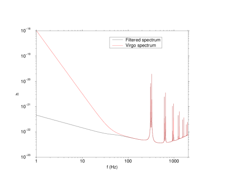
Figure 1: Virgo-like noise spectrum and the result after a pre-filtering which flattens the low frequency tail. Sampling frequency $f_{s}=4096\rm\,Hz$.

We need a pre-filtering of the low-frequency part of the spectrum, because the pendulum mode dominates the autocorrelation function. If we used adaptive algorithms to find the parameters of our spectrum model in such a way to follow the slow non stationarity of the noise, we would need a short learning time for the algorithms. This is an impossible task if we analyze a noise characterized by a long autocorrelation time.

1.1 Noise modeling as an AR process

We fit the spectrum showed in figure 1 by an autoregressive stochastic process of order $P$:

$$x_{n}=\sum_{k=1}^{P}a_{k}x_{n-k}+\sigma\xi_{n}$$ (7)

where $\xi_{n}$ are independent normal random numbers and $a_{k}$ are the $P$ parameters of the model.

The relationship between the parameters of the model and the autocorrelation function $r_{xx}(n)$ is given by the Yule–Walker equations

$$r_{xx}(n)=\left\{\begin{array}[]{ll}\sum_{k=1}^{p}a_{k}r_{xx}(n-k)&\mbox{for}\ n\geq 1\\ \sum_{k=1}^{p}a_{k}r_{xx}(-k)+\sigma^{2}&\mbox{for}\ n=0\end{array}\right.$$ (8)

Given the spectrum, we obtain the autocorrelation function and we can solve for the coefficients $\{a_{k}\}$ by the Durbin algorithm [1].

The key point is to find the optimal value $P$ for the order of the process. In literature there are some standard criteria which may be used in order to determine this value. We have tested the Akaike information criterion (AIC), the Minimum description length (MDL) and the Akaike final prediction error (FPE): the MDL criterion is the most efficient among them in finding a minimum. It reaches a minimum value for $P=292$.

We choose to fit the filtered noise spectrum with an $AR(292)$ model and to generate the data sample on which we shall perform the adaptive test with the AR parameters estimates with the Durbin algorithm. The result of the fit is shown in figure 2. Once we found the reflection parameters [1] with Durbin algorithm we can implement the associated linear predictor in the time domain and in the lattice fashion [1]. The output of this whitening filter in shown in figure  2.

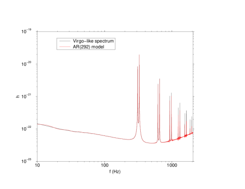
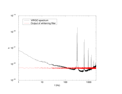
Figure 2: On the left: AR(292) model fit to the spectrum. On the right: input and output of a Durbin whitening filter

2 Adaptive identification of AR parameters

We have just seen how to implement a whitening filter if we use the Durbin algorithm to compute the reflection coefficients of our process. Now, we want to estimate these coefficients on line without estimating the correlation function first, but directly from the input data. There are several ways of accomplishing this purpose. We have tested some of the most popular algorithms, which can be divided in two main categories: the gradient methods (GAL) and the least squares methods (LS) In the gradient based methods we use an estimate of the cost function at the $n$th step which is based on the $n$th data input, while the updating criterion for the learning parameter is derived by minimizing the expectation value of the cost function. On the other hand, in the least squares based methods the optimal least squares prediction is computed at every point in time keeping into account the whole data history.

2.1 Results

We report in figure 3 the results obtained with the Least Squares Lattice (LSL) filter which is the best working among the algorithms we analyzed. It is evident the efficiency of this algorithm in following all the features of the noise spectrum.

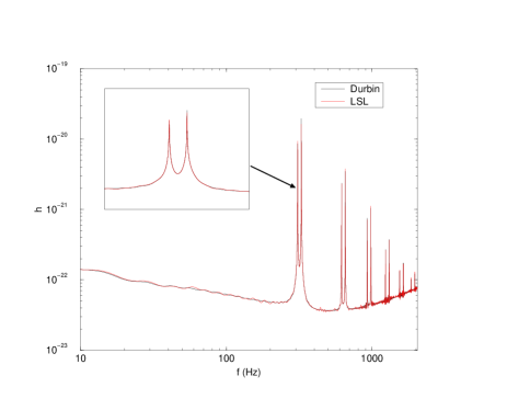
Figure 3: LSL fit to AR(292) spectrum. Input and output of a LSL filter.

The fast convergence of the algorithm lets us follow non stationarity of the noise which are slower than one minute. To check the quality of an estimator we need to put a bound on its performance. We can use general results from the theory of statistical estimators. The variance of any unbiased estimator is bounded from below by the Cramer-Rao bound. We checked if the variance of the AR parameters estimated with the LSL estimator attains these limits or not.

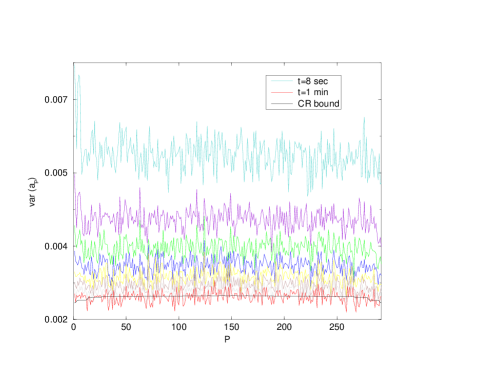
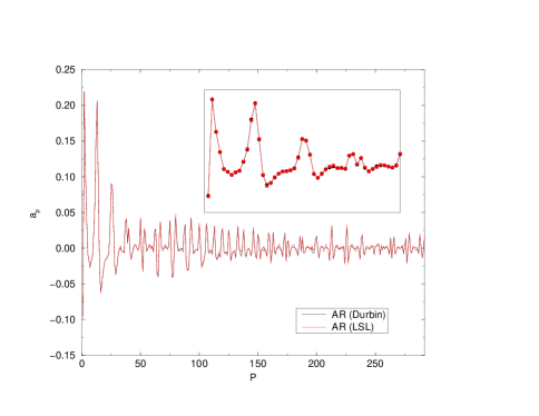
Figure 4: Cramer Rao lower bound. LSL fit to the AR parameters

We have computed the variance of each parameter and of $\sigma^{2}$ at different times to follow how the variance approaches the CR bound as time goes by. The times are delayed each other by $8$ seconds, the last time corresponding to one elapsed minute.

In Figure 4 we report the results. It is evident how the variance of each coefficient flattens to the CR limit as the number of iterations of the adaptive algorithm increases. After one minute of data input, the variance of the coefficients has already reached the CR bound. Therefore we conclude that the LSL estimator is an efficient one.

3 Conclusions

We have shown that it is possible to model a noise spectrum with complex features like those relevant for the VIRGO experiment by parameterizing it in terms of a small number of parameters.

We have tested some adaptive algorithms which are able to fit on line the parameters of an autoregressive representation of the VIRGO-like spectrum. The most efficient of them is the least squares lattice algorithm which, after one minute of data, converges and reproduces all the desired spectral features attaining moreover the Cramer Rao lower bound.

In principle, the fast convergence lets us follow the slow non stationarity of the noise. In a forthcoming note we shall describe in a detailed way the efficiency of the algorithm in dealing with non stationarities as a function of their characteristic time scales and amplitude magnitude.

References

References

- [1] S. Thomas Alexander, Adaptive signal processing, Springer, New York, 1986.
- [2] S. M. Kay, Modern spectral estimation, Prentice-Hall, Englewood Cliffs, New Jersey, 1995.
- [3] Charles W. Therrien, Discrete random signals and statistical signal processing, Prentice-Hall, Englewood Cliffs, 1992.