[

Chaos in the Einstein-Yang-Mills Equations

Abstract

Yang-Mills color fields evolve chaotically in an anisotropically expanding universe. The chaotic behaviour differs from that found in anisotropic Mixmaster universes. The universe isotropizes at late times, approaching the mean expansion rate of a radiation-dominated universe. However, small chaotic oscillations of the shear and color stresses continue indefinitely. An invariant, coordinate-independent characterisation of the chaos is provided by means of fractal basin boundaries.

]

Yang-Mills fields are central to quantum theories of elementary particles. They are of interest to dynamicists since they evolve chaotically in flat spacetime [1, 2, 3, 4]. But how do Yang-Mills fields behave in the early universe? Does the chaos persist, or is it eradicated by the general relativistic effects of cosmological expansion? The earliest studies of the Einstein-Yang-Mills (EYM) system assumed isotropic cosmological expansion. This imposes special symmetries on the dynamics and the dynamical system is integrable: chaos cannot exist [5]. Recently, a Yang-Mills theory was formulated in an axisymmetric, spatially homogeneous universe [6]. The large number of degrees of freedom made an analysis of the full dynamics difficult, and the coordinate dependence of the standard chaotic indicators meant that the relativistic chaos could not be invariantly characterised.

In this letter, we analyse general relativistic Yang-Mills chaos using invariant topological methods. We make the problem more tractable by an economical definition of variables, which reduces the dimension of the phase space substantially (from $8-D$ to $5-D$). In the physical picture that emerges, the asymptotic evolution of the spatial volume of the universe imitates a radiation-dominated universe, while the shear diminishes chaotically.

Previous studies of chaos in general relativity have focused on the non-axisymmetric Bianchi type VIII and IX (Mixmaster) universes, where the presence of anisotropic 3-curvature creates an infinite sequence of chaotic oscillations on approach to an initial Weyl curvature singularity at $t=0$ [12, 13, 14]. This behaviour is intrinsically general relativistic. By contrast, the chaotic EYM cosmology that we study is different: chaos exists even when the metric is axisymmetric and the curvature is isotropic.

We evolve the Yang-Mills fields in the simplest anisotropic metrics of Bianchi type I. The color degrees of freedom of the Yang-Mills gauge fields oscillate chaotically, while the expansion attenuates their overall energy. The EYM action is

$$S=\int d^{4}x\sqrt{-g}\left[-{\frac{1}{16\pi G}}{\cal R}-{\frac{1}{4}}F_{\mu\nu}F^{\mu\nu}\right]\ \$$ (1)

where $F_{\mu\nu}$ is the gauge-invariant field strength. The spacetime is described by the axisymmetric Bianchi I metric, with scale factors $b(t)$ and $c(t)$:

$$ds^{2}=-dt^{2}+b^{2}(t)\left(dx^{2}+dy^{2}\right)+c^{2}(t)dz^{2}.$$ (2)

After fixing the internal gauge of the Yang-Mills field, the matter can be parametrized by two variables $(\alpha,\gamma)$ [6], which can be thought of as color degrees of freedom for the massless gauge fields. The cosmological evolution is an orbit in the $(b,c,\alpha,\gamma)$ phase space.

We define the mean expansion scale factor by $a\equiv(b^{2}c)^{1/3},$ the shear anisotropy by $\chi\equiv(b/c)^{1/3}$, with volume expansion $H_{a}\equiv\dot{a}/a,$ and shear $H_{\chi}\equiv\dot{\chi}/\chi$. The scaled Yang-Mills field strengths will be defined by $(\Psi,\Gamma)\equiv(\alpha/(a\chi),\gamma\chi^{2}/a),$ with conjugate momenta $(\Pi_{\Psi},\Pi_{\Gamma})=(\dot{\alpha}/(a\chi),\dot{\gamma}\chi^{2}/a)$. The Einstein equations reduce to

$$\dot{H}_{a}+{\ 2}H_{a}^{2}+H_{\chi}^{2} = 0$$ (3)

$$\dot{H}_{\chi}-H_{\chi}^{2}+H_{a}^{2}+{3}H_{a}H_{\chi} = {\frac{1}{2}}\Psi^{4}+{\frac{1}{2}}\Pi_{\Gamma}^{2}\ \ .$$ (4)

The Hamiltonian constraint equation is

$${\frac{1}{2}}\Pi_{\Gamma}^{2}+\Pi_{\Psi}^{2}+{\frac{1}{2}}\Psi^{4}+\Psi^{2}\Gamma^{2}=3\left(H_{a}^{2}-H_{\chi}^{2}\right)\ \ .$$ (5)

The conservation of gravitational-plus-matter energy appears in the ($\Psi,\Gamma$) subsystem as a loss of energy, given by $E(t)=3(H_{a}^{2}-H_{\chi}^{2})$. The matter conservation equations are

$$\dot{\Pi}_{\Psi}+2(H_{a}+H_{\chi})\Pi_{\Psi}+\Psi\left(\Gamma^{2}+\Psi^{2}\right) = 0$$ (6)

$$\dot{\Pi}_{\Gamma}+2(H_{a}+H_{\chi})\Pi_{\Gamma}+2\Psi^{2}\Gamma = 0\ .$$ (7)

The matter sector is thus a driven, dissipative system. The Yang-Mills coordinates decay adiabatically due to the expansion, but they are also driven by oscillations in $H_{\chi}$.

There are 4 coordinates, $(H_{a},H_{\chi},\Psi,\Gamma),$ and 8 degrees of freedom. This system permits at most $4$ positive Lyapunov exponents. However, eqns (3) and (4) are constraints. Consequently, only $6$ constants of integration need be specified. The Hamiltonian constraint reduces this by one, leaving $5$ degrees of freedom. If each of the three constraint equations are unique, then there is only one positive Lyapunov exponent, as in flat spacetime ($H_{a}=H_{\chi}=0)$. This is to be expected since the vacuum Bianchi I universe is integrable. Any chaos in the metric variables is therefore a consequence of chaos in the Yang-Mills field. This was also found to be the case in Ref. [9].

The color amplitudes of the Yang-Mills system scatter around the potential of Fig. 1. The chaos is more complicated than that found in Mixmaster universes because of the rapidly varying curvature of the hyperbolic potential walls. In flat spacetime the energy remains constant, and the contours define different surfaces of constant energy. In the Bianchi I universe of general relativity, $E(t)$ drops asymptotically (see eqn (5)). The four hyperbolic potential walls shrink as the energy available to the Yang-Mills field decays. We see from Fig. 2, the trajectories occupy smaller and smaller volumes of the matter phase-space.

Chaos is often quantified by computing Lyapunov exponents. However, the values of Lyapunov exponents are coordinate dependent in general relativity [7], because of the coordinate covariance of Einstein’s equations (another manifestation of the so called ‘problem of time’ in cosmology). The authors of Ref. [6] cite this fact, together with the large number of degrees of freedom (which lead to Arnold diffusion) and the non-compact phase space, as major obstacles to a generalization of the study of chaotic properties of Yang-Mills theory to curved spacetimes. These barriers can be overcome by the methods of chaotic scattering [8, 9, 10, 11], which allow us to identify fractal sets which fully characterize the chaos. Fractals cannot be hidden by a reshuffling of coordinates: their existence and dimension are coordinate-independent topological features [8, 9, 10, 11]. The fractal set that we seek is the set of all periodic orbits: by analogy with the accessible states in thermodynamics, this periodic set completely describes the chaotic dynamics. The fractal set is also called a ‘strange repellor’, or ‘strange saddle’. If the global expansion of the universe could be projected out of the dynamical evolution, the repellor would consist of all periodic orbits trapped in the potential. When the global expansion is included, the periodic orbits are actually self-similar, reminiscent of the dynamics of the Bianchi IX cosmology [10, 12, 13, 14, 15, 16].

The strange repellor can be coded by a symbolic dynamics, or isolated directly by numerical techniques such as the PIM method. It is easier to employ the method of fractal basin boundaries. A slice of initial conditions is taken through phase space. All possible asymptotic states are determined and assigned a color (black or white here). If large blocks of initial data space suffer the same fate, then the outcome basin will look smooth and monochromatic; by contrast, highly mixed, fractalized basins indicate a sensitivity to initial conditions, as well as mixing and folding of trajectories. Hence, fractalized basins signal chaos in a covariant way. All observers agree upon the occurrence of the events used to construct the fractal, and all will agree on the dimension of the basin boundary.

A typical trajectory will travel down one of the $\Gamma$ channels before rebounding back into the scattering region of the potential. This is again reminiscent of the Mixmaster system, where the repellor was also inefficient [10]. In Mixmaster, the repelling set can be isolated by artificially opening the exit pockets, so that orbits thrown far from the scattering region were allowed to escape. Similarly, here, we cut holes in the pockets and assign the color white to the initial condition if the orbit falls down the upper pocket ($\Gamma>0$), and black if it falls down the lower pocket ($\Gamma<0$). In flat spacetime, this is straightforward. In the Bianchi I spacetime, the potential walls move inward as the energy is not constant. However, the same procedure can be followed, so that the angular size of the hole in the pocket is the same for all energy contours. Basin boundaries, sliced through $(\Psi,\Gamma)$ coordinates, are shown in Fig. 3. The pockets are of size $\theta=2\arctan 0.5$. The fractal basins look very similar to those we find in a flat spacetime. The box-counting dimension was estimated to be maximal, namely, $D_{o}=2$ (the same dimension as we found for the basins in flat spacetime). If the pockets are made infinitesimally thin, the fractal boundary fills all of phase space.

The interweaving of outcomes, demonstrated by the basin boundary structure, corresponds to a final-state sensitivity that is directly related to the fractal dimension. An $\epsilon$ uncertainty in initial values leads to a final-state uncertainty of $\epsilon^{N-D_{o}},$ where $N$ is the dimension of the phase space. In the $N=2$ slice of Fig. 3, we found $D_{o}=2$. Axisymmetric, Bianchi type I, EYM cosmologies are therefore very sensitive to initial conditions, and the shear evolution is highly chaotic.

The chaotic scattering has a subtle effect on the large-scale structure of the spacetime. In vacuum, the scale factor grows as $a\propto t^{1/3},$ and the shear is of comparable importance, $\chi\propto t^{1/3}$. The color oscillations scatter the metric variables chaotically. As the universe expands, the volume of the $(\Psi,\Gamma)$ phase space redshifts as $\rho\sim 1/a^{4}$. The scale factor eventually evolves towards the behaviour of a radiation-dominated universe, $a\sim t^{1/2},$ and is unaffected by the chaotic color oscillations. The relaxation timescale for this behaviour is related to the Lyapunov exponent, and hence to the fractal dimension [18]. A rough estimate indicates that trajectories attract onto $H_{a}=1/(2t)$ after a few e-folds of the scale factor. The shear is more vulnerable to stochastic behaviour and the color oscillations sustain oscillations of $H_{\chi}$ about zero. This general behaviour can be seen by examining the scattering angle in minisuperspace. A trajectory leaves the $(\ln a,\ln\chi)$ minisuperspace plane at an angle $\theta={\rm arctan}(H_{\chi}/H_{a})$. Fig. 4 compares the scattering angle in the case of regular motion to the angle in the chaotic case. The scattering angle is not constant in time as can be seen in Fig. 5. While $H_{a}$ escapes the effects of the chaotic scattering, $H_{\chi}$ remains sensitive and continues to oscillate.

The dependence of the final scattered angle on the impact parameter is a direct probe of the strange repellor. In a simple chaotic system, the scattering angle can become fractal. No matter how small a difference in the incident velocity, the difference in scattered angle is sizeable. The scattering angle and the basin boundaries are different ways of viewing the same phenomenon. Regardless, the scattering angle provides an important perspective. When the motion is regular, the angle approaches $\pm\pi/4$ and so $H_{\chi}\sim\pm H_{a}$. The evolution of the shear is as important as the global expansion of the spacetime volume, and initially the spacetime is highly anisotropic. At late times, under the influence of chaos, the scattering angle clusters about zero, and $|H_{\chi}|\ll H_{a}$, with the shear frozen at a nearly constant value. Since the field equations were shown to be invariant under a rescaling of the shear, we can choose that scale so that $\ln\chi\rightarrow 0$ at freeze out. Physically, this is equivalent to the statement that $a\sim b\sim c$. The anisotropy decays and the final state looks isotropic.

The chaotic behaviour influences the solution only through the second-order modes and the expansion of the volume behaves as if the universe is radiation dominated. This reveals a further connection between the chaotic behaviour in flat space-time and in expanding universes. If the energy-momentum tensor is trace-free, as it is for Yang-Mills fields, then any solution of the equations of motion in flat spacetime can be conformally rescaled to obtain a solution of the equations of motion in an isotropically expanding universe. This solution is approximate since it neglects the back-reaction of the motions on the space-time metric. Though we did not actually employ this approximate method, such a scaled solution would be an increasingly good description of the late-time behaviour, since isotropization occurs in that limit.

The global scale factor is fairly impervious to the buffeting of the other degrees of freedom. Small shear and color oscillations will continue forever, getting ever smaller in amplitude, and only asymptotically diluting to zero. We expect an infinite number of oscillations to occur to the future of any finite time. However on the coarsest scales, the universe evolves as though filled with radiation. Most interestingly, the original anisotropy is eroded and the universe appears isotropic.

JJL is especially grateful to N. Cornish and P. Ferreira for valuable discussions. JDB is supported by the PPARC and acknowledges support from the Center for Particle Astrophysics, Berkeley. JJL is supported in part by a President’s Postdoctoral Fellowship and acknowledges support from the PPARC at the Astronomy Centre, Sussex.

FIG. 1.: Isocontours of the color potential (eqn. (1.6)). As the energy, $E(t),$ decreases, the walls of the potential move inward and the color oscillations are confined accordingly. A typical trajectory is shown.

FIG. 2.: A projection of the Bianchi I phase space onto the $(\Psi,\Pi_{\Psi})$ plane (left) and onto the $(\Gamma,\Pi_{\Gamma}$) plane (right). The initial values for this trajectory are $\Psi=0.1,\Gamma=0,H_{a}=0.11,H_{\chi}=0.08,\dot{\Psi}=0$ and $\dot{\Gamma}$ is fixed by the Hamiltonian constraint, eq. (1.5).

A

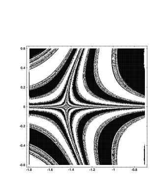
FIG. 3.: The strange repellor is revealed in these fractal basin boundaries. Holes are cut in the $\Gamma$ channels to allow typical trajectories to escape. The angular size of the pockets in this simulation is $\tan(\theta/2)=0.5$.

FIG. 4.: The scattering angle defined as $\theta={\rm arcsin}(H_{\chi}/H_{a})$ as a function of the initial $H_{a}$. The left plot is not chaotic with $\Psi=\dot{\Psi}=0$. In the right panel the initial conditions for the remaining degrees of freedom are $H_{\chi o}=0.0999$,$\Psi=0.1=-\Gamma=-\dot{\Psi}$. Again, the Hamiltonian constraint fixes $\dot{\Gamma}$.

B

FIG. 5.: The scattering angle as a function of cosmic time. The initial conditions are $H_{a}=20.0002,20.000245,20.00026$, $H_{\chi}=0.0999$,$\Psi=0.1=-\Gamma=-\dot{\Psi}$. The scattering angle as a function of cosmic time corresponding to the regular dip seen in the above blow up in Fig. 4. On the right, the initial conditions are $H_{a}=20.00026$,$20.000265$,$20.0002675$, $H_{\chi}=0.0999$,$\Psi=0.1=-\Gamma=-\dot{\Psi}$. The Hamiltonian constraint fixes $\dot{\Gamma}$.

REFERENCES

- [1] G.Z.Baseyna, S.G. Matinyan, and G.K. Savvidi, JETP Lett. 29, 585 (1979).
- [2] S.G. Matinyan, G.K. Savvidi, and N.G.Ter-Arutyunyan-Savvidi, Sov. Phys. JETP 53, 421 (1981).
- [3] B.V. Chirikov and D.L. Shepelyanskii, JETP Lett. 34, 164 (1981).
- [4] B.V. Chirikov and D.L. Shepelyanskii, Sov. J. Nucl. Phys. 36, 908 (1982).
- [5] D.V. Galt’sov and M.S. Volkov, Phys. Lett. B 256, 17 (1991).
- [6] B.K. Darian and H.P. Künzle, Class. Quantum Grav. 12 (1995) 2651.
- [7] S. E. Rugh, Cand. Scient. Thesis, The Niels Bohr Institute, (1990).
- [8] C. P. Dettmann, N. E. Frankel and N. J. Cornish, Phys. Rev. D50, R618 (1994); Fractals, 3, 161 (1995).
- [9] N. J. Cornish and J. J. Levin, Phys. Rev. D53, 3022 (1996).
- [10] N. J. Cornish and J. J. Levin, Phys. Rev. Lett. 1997.; N. J. Cornish and J. J. Levin, to be published in Phys. Rev. D.
- [11] N. J. Cornish and G. Gibbons, to be published, gr-qc/9612060.
- [12] C. W. Misner, Phys. Rev. Lett. 22, 1071, (1969).
- [13] I. M. Khalatnikov & E. M. Lifshitz, Phys. Rev. Lett. 24, 76 (1970); V. A. Belinskii, I. M. Khalatnikov & E. M. Lifshitz, Adv. Phys. 19, 525 (1970).
- [14] J. D. Barrow, Phys. Rev. Lett. 46, 963 (1981); Phys. Rep. 85, 1 (1982); Gen. Rel. Gravitation, 14, 1523 (1982); D. F. Chernoff & J. D. Barrow, Phys. Rev. Lett. 50, 134 (1983); J.D. Barrow, in Classical General Relativity, eds. W. Bonnor, J. Islam, and M.A.H. MacCallum, Cambridge UP, Cambridge, (1984), pp. 25-41.
- [15] B. K. Berger, Gen. Rel. Grav. 23, 1385 (1991); Phys. Rev. D47, 3222 (1993).
- [16] D. Hobill, A. Burd & A. Coley, eds.Deterministic chaos in general relativity, (Plenum Press, New York, 1994) references therein.
- [17] E. Ott, Chaos in dynamical systems, (Cambridge UP, Cambridge, 1993).
- [18] Since the fractal dimension codifies the loss of information it is sensible that the Lyapunov exponent determined in any gauge must be intimately connected with this dimension. In fact it has been conjectured that the information dimension of the repellor is directly related to the Lyapuov dimension, a gauge invariant combination of the Lyapunov exponent and the time scale of the chaotic transient [19, 20, 21, 22]. For a demonstration of the equivalence in relativity see Ref. [10].
- [19] J. L. Kaplan and J. A. Yorke, in Functional differential equations and approximations of fixed points eds. H. O. Peitgen and H. O. Walter, (Springer, Berlin, 1979).
- [20] C. Grebogi, E. Ott, J. A. Yorke, Phys. Rev. A. 37, 1711 (1988).
- [21] L. S. Young, Ergod. Th. Dynam. Syst. 2, 109 (1982); A. Fathi, Commun. Math. Phys. 126, 249 (1989).
- [22] H. Kantz and P. Grassberger, Physica D 17, 75 (1985); T. Bohr and D. Rand, Physica D 25, 387 (1987); G. H. Hsu, E. Ott and C. Grebogi, Phys. Lett. A127, 199 (1988). Z. Kovacs and L. Wiesenfeld, Phys. Rev. E51, 5476 (1995)
A
B