General-relativistic coupling between orbital motion and internal degrees of freedom for inspiraling binary neutron stars.

Abstract

We analyze the coupling between the internal degrees of freedom of neutron stars in a close binary, and the stars’ orbital motion. Our analysis is based on the method of matched asymptotic expansions and is valid to all orders in the strength of internal gravity in each star, but is perturbative in the “tidal expansion parameter” (stellar radius)/(orbital separation). At first order in the tidal expansion parameter, we show that the internal structure of each star is unaffected by its companion, in agreement with post-1-Newtonian results of Wiseman (gr-qc/9704018). We also show that relativistic interactions that scale as higher powers of the tidal expansion parameter produce qualitatively similar effects to their Newtonian counterparts: there are corrections to the Newtonian tidal distortion of each star, both of which occur at third order in the tidal expansion parameter, and there are corrections to the Newtonian decrease in central density of each star (Newtonian “tidal stabilization”), both of which are sixth order in the tidal expansion parameter. There are additional interactions with no Newtonian analogs, but these do not change the central density of each star up to sixth order in the tidal expansion parameter. These results, in combination with previous analyses of Newtonian tidal interactions, indicate that (i) there are no large general-relativistic crushing forces that could cause the stars to collapse to black holes prior to the dynamical orbital instability, and (ii) the conventional wisdom with respect to coalescing binary neutron stars as sources of gravitational-wave bursts is correct: namely, the finite-stellar-size corrections to the gravitational waveform will be unimportant for the purpose of detecting the coalescences.

I INTRODUCTION AND SUMMARY

Recent numerical simulations by Wilson, Mathews and Marronetti of the late stages of inspiral of neutron star binaries have predicted the following surprising result: The individual neutron stars are apparently subject to a crushing force of general-relativistic origin which can cause the stars to collapse and form black holes, before they reach the dynamical orbital instability that marks the end of the inspiral [1, 2]. These numerical simulations were fully relativistic, but assumed a conformally flat spatial metric, and also employed an approximation scheme in which the gravitational field was constrained to be time-symmetric at each time-step in the computation. These approximations and assumptions give correct results for spherically symmetric systems and also to the first post-Newtonian approximation [3]; beyond this, however, their domain of validity is not well understood.

The Wilson-Mathews-Marronetti prediction is in disagreement with other, independent, fully relativistic, numerical simulations which employ similar approximations [4, 5], with post-1-Newtonian numerical simulations [6], and with Post-Newtonian [7, 8, 9] and perturbation [10] calculations, which we discuss further below. Therefore it seems likely that star crushing does not occur in reality, although the issue is still somewhat controversial.

The star-crushing scenario, if correct, would have profound implications for the efforts to detect gravitational waves produced by neutron star inspirals with ground based interferometers such as LIGO and VIRGO [11]. A crushing force which is strong enough to cause an instability to radial collapse of a neutron star would constitute a strong coupling between the orbital motion and the internal modes of each star [12], and would transfer a substantial amount of energy from the orbital motion to each star. Specifically, let $L_{\rm instability}$ be the value of the orbital separation $L$ at the onset of instability, let $R$ be the initial radius of the neutron star, and let $\Delta R$ be the amount by which the star’s radius is decreased before the instability occurs. Then the ratio of the energy $\Delta E_{\rm star}$ absorbed by the neutron star [13] to the energy $\Delta E_{\rm gw}$ radiated in gravitational waves between $L=L_{\rm instability}/2$ and $L=L_{\rm instability}$ would be approximately

$${\Delta E_{\rm star}\over\Delta E_{\rm gw}}\sim\left({L_{\rm instability}\over R}\right)\,\left({\Delta R\over R}\right).$$ (1)

The Wilson-Mathews-Marronetti simulations predict that an instability occurs at $L_{\rm instability}\sim 5R$, and that $\Delta R/R\sim 1/20$ [14]. Therefore the ratio (1) is predicted to be of order unity, and the crushing effect gives rise to an order unity perturbation to the inspiral rate of the orbit and to the phase evolution of the emitted gravitational waves [15]. Since high accuracy theoretical templates are required in order to extract the signal from detector noise, the star-crushing scenario would imply that currently envisaged search templates [16] (which are calculated neglecting all orbital-motion—internal-mode couplings) would need to be completely revised. Therefore, it is important to find out whether or not the star crushing effect occurs.

In the Newtonian approximation, the coupling between the stars’ orbital motions and their internal motions has been analyzed in detail [17, 18, 19, 20, 21, 22]. The Newtonian coupling is very weak, too weak to affect the gravitational wave signal except in the last few orbits before coalescence [17, 18, 19, 20, 21, 22]. Moreover, the Newtonian interaction energy is $2-3$ orders of magnitude smaller at $L\sim 5R$ than the amount (1) which would be required to crush neutron stars when the necessary $\Delta R/R$ is of order several percent [7, 14]. Although post-Newtonian couplings have not yet been analyzed in detail [23], the expectation has generally been that post-Newtonian or relativistic couplings would simply be of the form (Newtonian coupling) $\times$ $\ O(M/R)$ or $O(M/L)$, where $M$ is the neutron star mass. That is, only small fractional corrections to existing Newtonian couplings are expected. However, the Wilson-Mathews-Marronetti prediction suggested instead that relativistic couplings could dominate over the Newtonian ones, and highlighted the need to understand the details of these couplings. The purpose of this paper is to explore and elucidate the relativistic, post-Newtonian couplings.

In the simulations of Wilson, Matthews and Marronetti [1], the central density $\rho_{c}$ of each star was seen to increase during the inspiral, and the instability to radial collapse occurred once the fractional increase in central density reached a few percent. In this paper, we shall not consider the issue of stability to radial collapse, but instead, following Refs. [8, 10], we shall focus attention on how the central density changes during the inspiral. Focusing on the central density allows us to investigate the existence of radial crushing forces (which presumably cause the instability to collapse in the simulations).

A Relativistic coupling between orbital motion and internal degrees of freedom in neutron star binaries

For a neutron star in a binary system, let $L$, $R$ and $M$ be the orbital separation, stellar radius and stellar mass, respectively. Then, there are two natural, independent, dimensionless parameters that characterize the system: the strength of internal gravity in each star

$$\epsilon\equiv{M\over R},$$ (2)

which is of order $\sim 0.2$, and the tidal expansion parameter

$$\alpha\equiv{R\over L}$$ (3)

which gradually increases during the inspiral. In terms of these parameters, the post-Newtonian expansion parameter for the orbital motion is $\epsilon_{\rm orbit}=M/L=\epsilon\alpha$. The standard post-Newtonian approximation scheme consists of expanding in $\epsilon$ and $\epsilon_{\rm orbit}$, treating these quantities as formally of the same order. In the context of a neutron star binary, the usual terminology for describing the size of gravitational effects (Newtonian, Post-1-Newtonian, Post-2-Newtonian etc.) is somewhat ambiguous, since an effect of post-$n$-Newtonian order could scale as $\epsilon^{a}(\alpha\epsilon)^{b}$ for any $a$, $b$ with $a+b=n$. In addition, some authors would classify an interaction which scales like $\epsilon^{s}\alpha^{t}$ as being of effective post-Newtonian order $t$, irrespective of the value of $s$, since the index $t$ controls the perturbation to the phase evolution of the emitted gravitational waves. Therefore, in this paper we will not use the post-Newtonian terminology.

Let us start by reviewing the situation in Newtonian gravity, at order $\epsilon^{0}$ (see Table I below). As is well known, each star distorts the other at $O(\alpha^{3})$ via the quadrupole tidal interaction, and the second order response of each star to the quadrupole tidal field of its companion gives rise to a decrease in its central density $\rho_{c}$ at $O(\alpha^{6})$ [7]. Each star expands slightly and thus becomes more stable against radial collapse [7].

Consider now the situation at higher orders in $\epsilon$. If there were a relativistic crushing force that changed the central density of each star, then this change in density $\delta\rho_{c}$ would scale in some way with the dimensionless parameters $\alpha$ and $\epsilon$:

$${\delta\rho_{c}\over\rho_{c}}\propto\alpha^{t}\,\epsilon^{s},$$ (4)

for some integers or half-integers $s,t>0$. Such an effect would dominate over the Newtonian effect at large orbital separations if $t<6$. Note that naive arguments (which turn out to be incorrect) do suggest scalings of the form (4) with low powers of $\alpha$ [24]. In the numerical simulations it was seen that $\delta\rho_{c}/\rho_{c}\propto\alpha^{2}$ [2], while the scaling with $\epsilon$ was not clear. A post-1-Newtonian calculation by Wiseman [8] has shown that there is no change in $\rho_{c}$ at the order $O(\alpha\,\epsilon)$, but did not rule out the possibilities $\delta\rho_{c}/\rho_{c}\propto\epsilon\,\alpha^{t}$ with $1<t<6$, or $\delta\rho_{c}/\rho_{c}\propto\epsilon^{s}\,\alpha$ with $s>1$.

A different approximation scheme was used by Brady and Hughes to investigate relativistic interactions [10]. Suppose that the two stars are labeled A and B, and that their masses and radii are $M_{A}$, $M_{B}$, $R_{A}$ and $R_{B}$. Brady and Hughes showed using perturbation theory that there is no change in the central density of star A to linear order in $M_{B}$. However, this result would not rule out a change in central density scaling as, for example,

$${\delta\rho_{c}\over\rho_{c}}\ \propto\ {M_{A}M_{B}^{2}\over R_{A}L^{2}}.$$ (5)

If we specialize to the equal mass case $M_{A}=M_{B}$ and $R_{A}=R_{B}$, the scaling (5) reduces to $\delta\rho_{c}/\rho_{c}\ \propto\ \epsilon\alpha^{2}$. Thus, the Brady-Hughes analysis does not necessarily rule out the type of behavior seen in the numerical simulations.

In this paper we analyze the change in central density to all orders in $\epsilon$, but perturbatively in $\alpha$. We show that in a binary system, the excitation of the internal degrees of freedom of a fully relativistic spherical star is qualitatively the same as that of a Newtonian star. At order $O(\alpha^{3})$, the star responds linearly to the external gravitational field, and is distorted; but there is no excitation of the stars spherically symmetric, radial modes. At order $O(\alpha^{6})$, the second-order response of the star to the external field generates an excitation of the stars spherically symmetric modes and a corresponding change in central density. We deduce that to all orders in $\epsilon$, any changes in central density must scale in the same way as in Newtonian theory:

$${\delta\rho_{c}\over\rho_{c}}\,\propto\,\alpha^{6}$$ (6)

as $\alpha\to 0$; see Table I below. Our result is restricted by the assumption that the neutron stars are not spinning. This restriction is unimportant since in Ref. [2] the crushing effect is seen when the neutron stars have very small net spins. Note that the result (6) is not based on an analysis that includes “only tidal interactions”. Instead, our analysis is a demonstration that there are no general-relativistic interactions that contribute to the leading-order change in central density other than the Newtonian-type tidal interactions.

Our result (6) is in disagreement with Refs. [1, 2] in the regime $\alpha\ll 1$ where there should be agreement: Fig. 1 of Ref. [2] shows that the scaling found in the numerical simulations is $\delta\rho_{c}/\rho_{c}\propto\alpha^{2}$ as $\alpha\to 0$. This disagreement in scaling strongly suggests that the star crushing effect seen in Refs. [1, 2] is not physical.

Our derivation of the result (6) takes place in two stages. First, in Secs. II, III and IV, we analyze the change in central density for a star moving in a fixed, external, vacuum gravitational field. We show that in this context $\delta\rho_{c}$ scales as ${\cal R}^{-4}$, where ${\cal R}$ is the radius of curvature of the external spacetime [cf. Eq. (130) below]. In Sec. V we extend the analysis to two stars in a binary, and deduce the scaling (6).

We use units in which the speed of light $c$ and Newton’s gravitational constant $G$ are unity, and use the sign conventions of Ref. [29]. Indices $a,b,c,\ldots$ will be abstract spacetime indices in the sense of Wald [30], thus equations involving such indices will be valid in all coordinate systems. Indices $\alpha$, $\beta$, $\gamma,\ldots$ and $i,j,k,\ldots$ will be conventional indices, the former running over $0,1,2,3$, the latter running over $1,2,3$.

II INTERACTIONS OF A FREELY FALLING BODY WITH AN EXTERNAL GRAVITATIONAL FIELD

In this section and in the following two sections we shall consider a neutron star moving in some arbitrary background vacuum gravitational field, for example a supermassive black hole. The key technical tool in our analysis is the method of matched asymptotic expansions, as explained in, for example, Refs. [25, 26, 27]. This method has been used in the past in general relativity primarily to derive equations of motion for bodies moving in external gravitational fields [26, 27]. However, the method also lends itself naturally to analyzing the effect of an external gravitational field on the internal structure of a fully relativistic, self-gravitating body. The key feature of the matched asymptotic expansion method is a separation of lengthscales/timescales: the radius of curvature of the external spacetime is assumed to be much larger than the lengthscales characterizing the neutron star, and the timescales over which the external curvature is changing (as perceived on the neutron star’s worldline) is much longer than the internal dynamical timescale of the neutron star.

The methods and result which we discuss in this section and in Secs. III and IV below do not apply directly to two stars of comparable mass in a binary, since in that context there is no external, fixed, background gravitational field. In Sec. V we show how to mesh the matched asymptotic expansion method with the post-Newtonian expansion method, and extend our analysis to be applicable to two stars in a binary. The discussion of motion in fixed external gravitational field of Secs. II – IV is included as background and motivation for the analysis of Sec. V.

A Constructing the spacetime: setup

Let the metric of the background field (for example, the supermassive black hole) be $g_{ab}^{(B)}$, and suppose that there are no matter sources in the region of interest in the background spacetime, i.e., it is a solution of the vacuum Einstein equations. Suppose also that $\Gamma$ is some geodesic in this spacetime. Then, one can pick Fermi-normal coordinates ${\bar{x}}^{\alpha}=({\bar{t}},{\bar{x}}^{i})$ adapted to this geodesic, such that $\Gamma$ is the curve ${\bar{x}}^{i}=0$, and such that the metric is of the form

$$g_{ab}^{(B)}={\bar{\eta}}_{ab}+h^{(B)}_{ab}$$ (7)

where ${\bar{\eta}}_{ab}$ is the flat, Minkowski metric ${\bar{\eta}}_{ab}=-(d{\bar{t}})_{a}(d{\bar{t}})_{b}+\delta_{ij}(d{\bar{x}}^{i})_{a}(d{\bar{x}}^{j})_{b}$, and where $h^{(B)}_{ab}$ is quadratic in distance from the geodesic. More specifically, near the geodesic $\Gamma$ we have [28]

$$h^{(B)}_{\alpha\beta}d{\bar{x}}^{\alpha}d{\bar{x}}^{\beta} = -R_{0l0m}{\bar{x}}^{l}{\bar{x}}^{m}\,d{\bar{t}}^{2}-{4\over 3}R_{0ljm}{\bar{x}}^{l}{\bar{x}}^{m}\,d{\bar{t}}d{\bar{x}}^{j}$$ (9)

$$-{1\over 3}R_{iljm}{\bar{x}}^{l}{\bar{x}}^{m}\,d{\bar{x}}^{i}d{\bar{x}}^{j}\,+O(|{\bar{x}}^{i}|^{3}),$$

where the various Riemann tensor components are evaluated at $({\bar{t}},{\bar{x}}^{i})=({\bar{t}},0)$, i.e., on $\Gamma$.

We next introduce some notation. Let ${\cal R}_{c}$ denote the order of magnitude of the radii of curvature of the background spacetime along $\Gamma$, so that ${\cal R}_{c}^{-2}=$ typical value of the Riemann tensor components on the right hand side of Eq. (9). Let ${\cal L}$ and ${\cal T}$ be the lengthscale and timescale, respectively, over which the curvature is changing, given schematically by $R_{\alpha\beta\gamma\delta}/{\cal L}\sim\nabla_{i}R_{\alpha\beta\gamma\delta}$ and $R_{\alpha\beta\gamma\delta}/{\cal T}\sim\nabla_{0}R_{\alpha\beta\gamma\delta}$. Below we will treat ${\cal R}_{c}$, ${\cal L}$ and ${\cal T}$ as formally of the same magnitude, and will denote these lengthscales collectively by ${\cal R}$.

Consider now a completely different spacetime: a static, spherical, isolated neutron star, which we model as a perfect fluid obeying some equation of state $p=p(\rho)$ [31]. Let its mass be $M$ and its Schwarschild radius be $R$. In a suitable coordinate system $x^{\alpha}=(t,x^{i})$, the neutron star metric can be written as

$$g_{ab}^{({\rm NS})}=\eta_{ab}+h^{({\rm NS})}_{ab},$$ (10)

where ${\eta}_{ab}=-(dt)_{a}(dt)_{b}+\delta_{ij}(dx^{i})_{a}(dx^{j})_{b}$, $r=\sqrt{\delta_{ij}x^{i}x^{j}}$, and at large $r$

$$h^{({\rm NS})}_{\alpha\beta}dx^{\alpha}dx^{\beta} = -\left[-2M/r+2M^{2}/r^{2}\right]\,dt^{2}$$ (13)

$$+\left[{2M\over r}+{3M^{2}\over 2r^{2}}\right]\delta_{jk}dx^{j}dx^{k}$$

$$+O\left({1\over r^{3}}\right).$$

The task now is to construct, starting from the metrics (7) and (10), an approximate solution of Einstein’s equations that represents the neutron star traveling along the curve $\Gamma$ in the background spacetime, in the limit where $R\ll{\cal R}.$ In Sec. II B we describe, without proof, the resulting spacetime to lowest order in the dimensionless parameters

$$\gamma_{1}=R/{\cal R}$$ (14)

and

$$\gamma_{2}=M/{\cal R}.$$ (15)

This leading order spacetime is well known. Then, starting in Sec. II C we describe a systematic procedure for calculating the spacetime metric to successive orders in the parameters (14) and (15) [26, 27], which can be used to verify the results of Sec. II B. Finally in Sec. IV we deduce the scaling of the change in central density of the star.

B The leading order spacetime

Consider the region $R\ll r\ll{\cal R}$ in the background spacetime (9), which we will call the matching region. In this region, consider the metric

$$g_{ab}^{({\rm MATCHING})}=\eta_{ab}+h_{ab}^{({\rm NS})}+h_{ab}^{(B)}$$ (16)

obtained by identifying the coordinates used in Eqs. (9) and (13) and by simply adding the metric perturbations. The superscript (MATCHING) indicates the region of spacetime in which the expression is valid. The metric (16) is an approximate solution of the vacuum Einstein equation in the matching region, since $h_{ab}^{({\rm NS})}$ and $h_{ab}^{(B)}$ are both approximate solutions of the linearized vacuum Einstein equation. To leading order in the dimensionless expansion parameters (14) and (15), the metric (16) is the correct, physical metric in the matching region.

What of outside the matching region? The physical metric of the spacetime, again to leading order in the tidal expansion parameters, can be obtained as follows. In the region $r\sim R$, which we will call the interior region, the metric is

$$g_{ab}^{({\rm INTERIOR})}=\eta_{ab}+h_{ab}^{({\rm NS})}+{\hat{h}}_{ab}^{(B)}.$$ (17)

Here, the tensor $h_{ab}^{({\rm NS})}$ is the full, nonlinear metric perturbation of the neutron star. The tensor ${\hat{h}}_{ab}^{(B)}$ is a linearized metric perturbation which describes the leading order effect of the external tidal field. This metric perturbation, together with some linearized perturbation to the star’s fluid variables, is a solution of the coupled Einstein plus perfect fluid equations, linearized about the neutron star background, and with all time derivative terms dropped [32]. [The time derivative terms scale as $1/{\cal T}\sim 1/{\cal R}$ and thus enter at higher order in the small parameters (14) and (15); see Sec. II C below and Ref. [25].] The solution ${\hat{h}}_{ab}^{(B)}$ is chosen such that, at large $r$, ${\hat{h}}_{ab}^{(B)}\to$ the quadratic expression on the right hand side of Eq. (9). These perturbations (of the metric and of the fluid variables) describe normal mode deformations [12] of the star responding adiabatically to the external tidal field. The boundary condition at large $r$ determines both the metric perturbation ${\hat{h}}_{ab}^{(B)}$ and the perturbations to the fluid variables. The situation is analogous to that in Newtonian gravity as analyzed in detail in Ref. [20], where the boundary condition on the Newtonian potential at large $r$ determines the solution of the stellar perturbation equations.

In a similar way, the spacetime metric in the exterior region $r\gtrsim{\cal R}$ can be written as

$$g_{ab}^{({\rm EXTERIOR})}={\bar{\eta}}_{ab}+{\hat{h}}_{ab}^{({\rm NS})}+h_{ab}^{(B)}.$$ (18)

Here, $h_{ab}^{(B)}$ is of order unity, and ${\hat{h}}_{ab}^{({\rm NS})}$ is a linearized solution of the vacuum Einstein equations on the background $g_{ab}^{(B)}$ in the exterior region, which matches smoothly onto $h_{ab}^{({\rm NS})}$ in the matching region. To leading order, ${\hat{h}}_{ab}^{({\rm NS})}$ is just the solution of the linearized vacuum Einstein equations on the background $g_{ab}^{(B)}$ whose source is a delta function along the worldline $\Gamma$.

C Constructing the spacetime: general method

In this section we describe a general scheme for calculating the spacetime metric perturbatively in the parameters (14) and (15), based on the treatment in Thorne and Hartle [26] and in Mino et. al. [27]. This general scheme justifies the claimed forms (17) and (18) above of the leading order metrics. It also enables us to go to higher order, which is necessary since (as in Newtonian and post-Newtonian theory) it turns out that changes in the central density of the star are quadratic in the leading order tidal field ${\hat{h}}_{ab}^{(B)}$. Therefore, in order to determine the leading order change in central density of the star, it is necessary to consider higher order perturbations which scale as $({\hat{h}}_{ab}^{(B)})^{2}$.

There are three elements to the general procedure: an internal scheme, an external scheme, and a matching of the two schemes [27].

1 The internal scheme

Let $(M^{({\rm NS})},g_{ab}^{({\rm NS})})$ denote the manifold and background metric (10) of the neutron star. The physical metric can be written as the background metric plus a sequence of perturbations of various orders, in a generalization of Eq. (17):

$$g_{ab}^{({\rm INTERIOR})} = g_{ab}^{({\rm NS})}+\varepsilon{\hat{h}}_{ab}^{(1)}+\varepsilon^{2}{\hat{h}}_{ab}^{(2)}+\varepsilon^{3}{\hat{h}}_{ab}^{(3)}$$ (20)

$$+\varepsilon^{4}{\hat{h}}_{ab}^{(4)}+O(\varepsilon^{5}).$$

Here ${\hat{h}}_{ab}^{(2)}$ is what we called ${\hat{h}}_{ab}^{(B)}$ above, and below we will show that ${\hat{h}}_{ab}^{(1)}=0$. The quantity $\varepsilon$ is a formal expansion parameter which can be set to one at the end of the calculation; each term $\varepsilon^{t}{\hat{h}}_{ab}^{(t)}$ scales like ${\cal R}^{-t}$ (but has no definite scaling with respect to $M$). We shall be working to order $O(\varepsilon^{4})$. The expansion (20) constitutes a general-relativistic generalization of the usual tidal expansion of stellar interactions in Newtonian gravity. In a similar way we can expand the stress-energy tensor $T_{ab}$ of the neutron star as

$$T_{ab}=T_{ab}^{(0)}+\varepsilon T_{ab}^{(1)}+\varepsilon^{2}T_{ab}^{(2)}+\varepsilon^{3}T_{ab}^{(3)}+\varepsilon^{4}T_{ab}^{(4)}+\ldots.$$ (21)

Here $T_{ab}^{(0)}$ is the stress-tensor of the static, spherical, unperturbed neutron star, and the higher order terms $\varepsilon^{t}T_{ab}^{(t)}$ scale as ${\cal R}^{-t}$.

The terms with $t=1$ in Eq. (20) and (21) actually vanish identically. This is because when one carries out the matching procedure described below to determine the solutions, one finds that there are no pieces of the internal solution that scale as ${\cal R}^{-1}$ [26]. Henceforth we shall anticipate this result and set ${\hat{h}}_{ab}^{(1)}=T_{ab}^{(1)}=0$.

Now the perturbations to the interior metric and to the neutron star are driven by the external gravitational fields which vary over a time scale ${\cal T}\sim{\cal R}\,\propto\,1/\varepsilon$. This fact needs to be built into the approximation scheme we use to derive the perturbation equations of motion. We can illustrate the nature of the required approximation scheme with the following example. Consider a scalar field $\Phi$ on flat spacetime obeying the equation

$$\Box\Phi=\left(-{\partial^{2}\over\partial t^{2}}+{\bf\nabla}^{2}\right)\Phi({\bf x},t)=\rho({\bf x},t),$$ (22)

where the source $\rho({\bf x},t)$ is of the form $\rho({\bf x},t)=\rho_{0}({\bf x},\varepsilon t)$, and the function $\rho_{0}$ is independent of $\varepsilon$. If we define $\Phi_{0}({\bf x},t)=\Phi({\bf x},t/\varepsilon)$ and $\tau=\varepsilon t$, Eq. (22) can be re-written as

$$\left(-\varepsilon^{2}{\partial^{2}\over\partial\tau^{2}}+{\bf\nabla}^{2}\right)\Phi_{0}({\bf x},\tau)=\rho_{0}({\bf x},\tau).$$ (23)

If $\rho_{0}$ is now specified as a power series in $\varepsilon$, we can solve for $\Phi_{0}$ order by order in $\varepsilon$ using Eq. (23). The equation of motion (23) can also be obtained (dropping the subscripts 0) simply by multiplying each time derivative in Eq. (22) by $\varepsilon$.

In a similar way, the equations of motion of the internal scheme can be obtained by writing out the Einstein and fluid equations in terms of the contravariant components $g_{ab}$ and $T_{ab}$ of the metric and stress tensor, substituting in the expansions (20) and (21), and by multiplying each time derivative by $\varepsilon$. More specifically, for each $\varepsilon$, there will exist an $\varepsilon$-dependent coordinate system $({\tilde{x}}^{i},{\tilde{t}})$ which varies smoothly in $\varepsilon$ and which coincides with the coordinate system $(x^{i},t)$ of Eq. (13) at $\varepsilon=0$, such that

$${\hat{h}}^{(t)}_{\alpha\beta}({\tilde{x}}^{i},{\tilde{t}})d{\tilde{x}}^{\alpha}d{\tilde{x}}^{\beta}={\tilde{h}}^{(t)}_{\alpha\beta}({\tilde{x}}^{i},\varepsilon{\tilde{t}})d{\tilde{x}}^{\alpha}d{\tilde{x}}^{\beta}$$ (24)

and

$$T^{(t)}_{\alpha\beta}({\tilde{x}}^{i},{\tilde{t}})d{\tilde{x}}^{\alpha}d{\tilde{x}}^{\beta}={\tilde{T}}^{(t)}_{\alpha\beta}({\tilde{x}}^{i},\varepsilon{\tilde{t}})d{\tilde{x}}^{\alpha}d{\tilde{x}}^{\beta}$$ (25)

for $t=1,2,3\ldots$. Here the tensors ${\tilde{h}}^{(t)}_{ab}$ and ${\tilde{T}}^{(t)}_{ab}$ are independent of $\varepsilon$. The Einstein and perfect fluid equations combined with Eqs. (20), (21), (24) and (25) now yield a system of equations for the tensors ${\tilde{h}}^{(t)}_{ab}$ and ${\tilde{T}}^{(t)}_{ab}$ analogous to Eq. (23). These equations will only be valid in the restricted class of coordinate systems for which the ansatz (24) and (25) are valid.

The approximation scheme can also be described in coordinate invariant terms in the following way. Let ${\tilde{t}}(\varepsilon)$ be a scalar field and ${\tilde{t}}^{a}(\varepsilon)$ a vector field with

$${\tilde{t}}^{a}\nabla_{a}{\tilde{t}}=1,$$ (26)

which reduce to the $t$ and $\partial/\partial t$ of the coordinate system (13) at $\varepsilon=0$. Define the tensor

$$\Lambda_{a}^{b}(\varepsilon)=\delta_{a}^{b}+\left({1\over\varepsilon}-1\right){\tilde{t}}^{b}\nabla_{a}{\tilde{t}}$$ (27)

Let $\chi_{\varepsilon}:M^{({\rm NS})}\to M^{({\rm NS})}$ be the mapping which moves any point $\ln\varepsilon$ units along integral curves of the vector field ${\tilde{t}}\,{\tilde{t}}^{a}$, i.e., in suitable coordinate systems $({\tilde{x}}^{i},{\tilde{t}})$, $\chi_{\varepsilon}$ maps $({\tilde{x}}^{i},{\tilde{t}})$ to $({\tilde{x}}^{i},\varepsilon{\tilde{t}})$. We make the following ansatz for the form of the metric $g_{ab}^{({\rm INTERIOR})}$ and the stress tensor $T_{ab}$:

$$g_{ab}^{({\rm INTERIOR})}(\varepsilon)=\Lambda_{a}^{c}(\varepsilon)\Lambda_{b}^{d}(\varepsilon)\,\chi_{\varepsilon\,*}{\tilde{g}}_{cd},$$ (28)

and

$$T_{ab}(\varepsilon)=\Lambda_{a}^{c}(\varepsilon)\Lambda_{b}^{d}(\varepsilon)\,\chi_{\varepsilon_{*}}{\tilde{T}}_{cd},$$ (29)

where

$${\tilde{g}}_{ab} = g_{ab}^{({\rm NS})}+\varepsilon{\tilde{h}}_{ab}^{(1)}+\varepsilon^{2}{\tilde{h}}_{ab}^{(2)}+\varepsilon^{3}{\tilde{h}}_{ab}^{(3)}$$ (31)

$$+\varepsilon^{4}{\tilde{h}}_{ab}^{(4)}+O(\varepsilon^{5})$$

and

$${\tilde{T}}_{ab}=T_{ab}^{(0)}+\varepsilon{\tilde{T}}_{ab}^{(1)}+\varepsilon^{2}{\tilde{T}}_{ab}^{(2)}+\varepsilon^{3}{\tilde{T}}_{ab}^{(3)}+\varepsilon^{4}{\tilde{T}}_{ab}^{(4)}+O(\varepsilon^{5}).$$ (32)

Here the tensors ${\tilde{h}}_{ab}^{(t)}$ and ${\tilde{T}}_{ab}^{(t)}$ are independent of $\varepsilon$ and $\chi_{\varepsilon\,*}$ is the pullback map. Equations (28) – (32) together with Eqs. (20) – (21) reduce to Eqs. (24) and (25) in suitable coordinate systems. [Note that the transformation in Eqs. (28) and (29) leave the background quantities $g_{ab}^{({\rm NS})}$ and $T_{ab}^{(0)}$ invariant.] Finally, the Einstein and perfect fluid equations

$$G_{ab}[g^{({\rm INTERIOR})}_{cd}] = 0$$ (33)

$$\mbox{}\nabla^{a}T_{ab} = 0,$$ (34)

when expanded order by order in $\varepsilon$, yield a system of elliptic equations for the tensors ${\tilde{h}}_{ab}^{(t)}$ and ${\tilde{T}}_{ab}^{(t)}$.

Below, we shall for simplicity set $\varepsilon=1$ after having derived the equations of motion. When $\varepsilon=1$ we have ${\tilde{h}}_{ab}^{(t)}={\hat{h}}_{ab}^{(t)}$ and ${\tilde{T}}_{ab}^{(t)}=T_{ab}^{(t)}$, and thus we can write the equations in terms of the fields ${\hat{h}}_{ab}^{(t)}$ and $T_{ab}^{(t)}$.

In order to write out explicitly the resulting equations of motion, we introduce the following notations. We define the operators $G_{ab}^{(1)}[h;g_{cd}^{({\rm NS})}]$ and $G_{ab}^{(2)}\left[h,h;g_{ab}^{({\rm NS})}\right]$, which act on metric perturbations and pairs of metric perturbations respectively, to be linear and quadratic parts of the Einstein tensor of the perturbed spacetime $g^{({\rm NS})}+\varepsilon h$:

$$G_{ab}[g^{({\rm NS})}+\varepsilon h] = G_{ab}[g^{({\rm NS})}]+\varepsilon G^{(1)}_{ab}[h;g^{({\rm NS})}]$$ (36)

$$+\varepsilon^{2}G^{(2)}_{ab}[h,h;g^{({\rm NS})}]+O(\varepsilon^{3}).$$

[Here and below we drop some of the tensorial indices for ease of notation]. We also use the expansions

$$G_{ab}^{(1)}[h]=G_{ab}^{(1,0)}[h]+G_{ab}^{(1,1)}[h]+G_{ab}^{(1,2)}[h]$$ (37)

and

$$G_{ab}^{(2)}[h,h]=G_{ab}^{(2,0)}[h,h]+G_{ab}^{(2,1)}[h,h]+G_{ab}^{(2,2)}[h,h],$$ (38)

where $G_{ab}^{(1,p)}$ and $G_{ab}^{(2,p)}$ scale as ${\cal T}^{-p}$, i.e., contain $p$ time derivatives, for $p=0,1,2$. We write the derivative operator for the metric $g_{ab}^{({\rm NS})}+\varepsilon h_{ab}$, for any perturbation $h_{ab}$, as

$$\nabla^{a}=\nabla^{(0)\,a}+\varepsilon\nabla^{(1)\,a}_{[h]}+\varepsilon^{2}\nabla^{(2)\,a}_{[h,h]}+O(\varepsilon^{3}).$$ (39)

This equation defines the operators $\nabla^{(1)\,a}_{[h]}$ and $\nabla^{(2)\,a}_{[h,h]}$, which are multiplicative and not differential operators despite the notation. Finally, we use the expansion

$$\nabla^{(t)\,a}=\sum_{p=0}\nabla^{(t,p)\,a},$$ (40)

for $t=0,1,2$, where $\nabla^{(t,p)\,a}$ contains $p$ time derivatives (either acting on $h$ or as differential operators) and thus scales as ${\cal T}^{-p}$.

Using these notations and the expansions (20) and (21), we obtain from Eq. (34) the perturbed fluid equations [31]

$$\nabla^{(0,0)\,a}T_{ab}^{(2)}+\nabla^{(1,0)\,a}_{[{\hat{h}}^{(2)}]}T_{ab}^{(0)}=0,$$ (41)

$$\nabla^{(0,0)\,a}T_{ab}^{(3)}+\nabla^{(1,0)\,a}_{[{\hat{h}}^{(3)}]}T_{ab}^{(0)}={\cal F}^{(3)}_{b},$$ (42)

and

$$\nabla^{(0,0)\,a}T_{ab}^{(4)}+\nabla^{(1,0)\,a}_{[{\hat{h}}^{(4)}]}T_{ab}^{(0)}={\cal F}^{(4)}_{b},$$ (43)

where the 4-force densities ${\cal F}^{(3)}_{b}$ and ${\cal F}^{(4)}_{b}$ are

$${\cal F}^{(3)}_{b}=-\nabla^{(1,1)\,a}_{[{\hat{h}}^{(2)}]}T_{ab}^{(0)}-\nabla^{(0,1)\,a}T_{ab}^{(2)}$$ (44)

and

$${\cal F}^{(4)}_{b} = -\nabla^{(1,2)\,a}_{[{\hat{h}}^{(2)}]}T_{ab}^{(0)}-\nabla^{(1,1)\,a}_{[{\hat{h}}^{(3)}]}T_{ab}^{(0)}-\nabla^{(0,1)\,a}T_{ab}^{(3)}$$ (46)

$$-\nabla^{(2,0)\,a}_{[{\hat{h}}^{(2)},{\hat{h}}^{(2)}]}T_{ab}^{(0)}-\nabla^{(1,0)\,a}_{[{\hat{h}}^{(2)}]}T_{ab}^{(2)}.$$

Note that the actual fluid equations of motion are obtained by using the formula $T_{ab}=(\rho+p)u_{a}u_{b}+pg_{ab}$, by assuming expansions of the form (21) for the density $\rho$ and four velocity $u^{a}$, and by substituting into Eqs. (41) – (43). However, the schematic form (41) – (43) will be sufficient for our purposes.

Similarly, from the Einstein equations we obtain the equations of motion for the metric perturbations ${\hat{h}}_{ab}^{(t)}$ for $m=2,3,4$ :

$$G_{ab}^{(1,0)}\left[{\hat{h}}^{(2)};g_{cd}^{({\rm NS})}\right]=8\pi T_{ab}^{(2)},$$ (47)

$$G_{ab}^{(1,0)}\left[{\hat{h}}^{(3)};g_{cd}^{({\rm NS})}\right]=8\pi T_{ab}^{(3)}-G_{ab}^{(1,1)}\left[{\hat{h}}^{(2)};g_{cd}^{({\rm NS})}\right],$$ (48)

and

$$G_{ab}^{(1,0)}\left[{\hat{h}}^{(4)};g_{cd}^{({\rm NS})}\right] = 8\pi T_{ab}^{(4)}-G_{ab}^{(1,1)}\left[{\hat{h}}^{(3)};g_{cd}^{({\rm NS})}\right]$$ (51)

$$-G_{ab}^{(2,0)}\left[{\hat{h}}^{(2)},{\hat{h}}^{(2)};g_{cd}^{({\rm NS})}\right]$$

$$-G_{ab}^{(1,2)}\left[{\hat{h}}^{(2)};g_{cd}^{({\rm NS})}\right].$$

Note that Eqs. (41) – (43) and also Eqs. (47) – (51) are elliptic and not hyperbolic.

As discussed in Sec. II B, Eqs. (41) and (47) for the leading order fields ${\hat{h}}_{ab}^{(2)}$ and $T_{ab}^{(2)}$ together describe a solution of the Einstein plus perfect fluid equations, linearized about the static neutron star background, with all time derivative terms dropped. The higher order equations (41), (42), (48) and (51) have the same basic structure, but contain additional source terms. We shall be interested in very general solutions of the equations which are allowed to diverge as $r\to\infty$; the physical solutions will be determined by matching to the metric of the external scheme.

2 The external scheme

Let $(M^{({\rm B})},g_{ab}^{({\rm B})})$ denote the manifold and metric (7) of the external spacetime. The physical metric can be written as this background metric plus a sequence of perturbations of various orders, in a generalization of Eq. (18):

$$g_{ab}^{({\rm EXTERIOR})} = g_{ab}^{({\rm B})}+\varepsilon{\bar{h}}_{ab}^{(1)}+\varepsilon^{2}{\bar{h}}_{ab}^{(2)}+O(\varepsilon^{3}).$$ (52)

Here as above $\varepsilon$ is a formal expansion parameter which can be set to one at the end of the calculation; in Eq. (52), each term $\varepsilon^{s}{\bar{h}}_{ab}^{(s)}$ scales like $M^{s}$ but has no definite scaling with respect to ${\cal R}$. [Here we treat the quantities $M$ and $R$ as formally of the same magnitude, so that the expansion parameters (14) and (15) coincide [33]]. The perturbation ${\bar{h}}_{ab}^{(1)}$ was denoted above as ${\hat{h}}_{ab}^{({\rm NS})}$. The equations of motion satisfied by the metric perturbations ${\bar{h}}_{ab}^{(1)}$ and ${\bar{h}}_{ab}^{(2)}$ are obtained from the vacuum Einstein equation:

$$G_{ab}^{(1)}\left[{\bar{h}}^{(1)};g_{cd}^{({\rm B})}\right] = 0$$ (53)

$$\mbox{}G_{ab}^{(1)}\left[{\bar{h}}^{(2)};g_{cd}^{({\rm B})}\right]+G_{ab}^{(2)}\left[{\bar{h}}^{(1)},{\bar{h}}^{(1)};g_{cd}^{({\rm B})}\right] = 0.$$ (54)

The solutions to these equations will diverge as ${\bar{r}}\to 0$, and will be determined by matching onto the internal solutions.

3 The matching scheme

In the matching region $R\ll r\ll{\cal R}$, the interior metric (20) can be written as the double expansion [33]:

$$g_{ab}^{({\rm INTERIOR})}=\eta_{ab}+\sum_{s=0}\,\sum_{t=0}\,{\hat{h}}_{ab}^{(s,t)}\,\left({M\over r}\right)^{s}\,\left({r\over{\cal R}}\right)^{t}.$$ (55)

Here the terms with $t=0$ are the expansion in powers of $M/r$ of the neutron star metric perturbation $h_{ab}^{({\rm NS})}$, and the terms with $t=1$ are the expansion in powers of $M/r$ of the metric perturbation ${\hat{h}}_{ab}^{(1)}$. The terms with $t=2$ give the expansion in powers of $M/r$ of the metric ${\hat{h}}_{ab}^{(2)}={\hat{h}}_{ab}^{(B)}$, which describes the leading order tidal gravitational field, and so forth. The form of the expansion (55) can be regarded as an ansatz which is validated by explicit matching calculations to the first few orders in $s$ and $t$ [27]; however, at higher orders in $s$ and $t$ it might be necessary to include powers of $(M/r)\log[M/r]$ or $(r/{\cal R})\log[r/{\cal R}]$ [34]. Moreover, the expansion is merely asymptotic and is not expected to be convergent [25]. From Eqs. (47) – (51), each term $h_{ab}^{(s,t)}(M/r)^{s}(r/{\cal R})^{t}$ in Eq. (55) obeys a linear elliptic equation with nonlinear source terms generated by the terms $h_{ab}^{(s^{\prime},t^{\prime})}(M/r)^{s^{\prime}}(r/{\cal R})^{t^{\prime}}$ with $s^{\prime}<s$ and/or $t^{\prime}<t$. The solutions for $t\geq 1$ diverge as $r\to\infty$.

In a similar way, we can perform a double expansion of the external metric (52):

$$g_{ab}^{({\rm EXTERIOR})}={\bar{\eta}}_{ab}+\sum_{s=0}\,\sum_{t=0}\,{\bar{h}}_{ab}^{(s,t)}\,\left({M\over{\bar{r}}}\right)^{s}\,\left({{\bar{r}}\over{\cal R}}\right)^{t},$$ (56)

where ${\bar{r}}^{2}=\delta_{ij}{\bar{x}}^{i}{\bar{x}}^{j}$. Here the terms of a given order $s$ give the expansion in powers of ${\bar{r}}/{\cal R}$ of the metric perturbation ${\bar{h}}_{ab}^{(s)}$, while the terms with $s=0$ are the expansion of the background metric $g_{ab}^{(B)}$.

The basic idea now is to demand consistency between the expansions (55) and (56). Before this can be done, however, one must specify an embedding

$$\varphi:\ M^{({\rm NS})}\to M^{({\rm B})},$$ (57)

of the neutron star spacetime into the external spacetime, i.e., a mapping between the asymptotically Lorentzian coordinates $x^{\alpha}$ of $M^{({\rm NS})}$ and the Fermi-normal coordinates ${\bar{x}}^{\alpha}$ of $M^{({\rm B})}$. Let us write this mapping as

$${\bar{x}}^{\alpha} = {\bar{x}}^{\alpha}(t,x^{i})$$ (58)

$$= \sum_{p=0}\,\left({M\over{\cal R}}\right)^{p}\,\sum_{r=0}\,\sum_{I_{r}}\ \ {}^{(r,p)}{\cal F}^{\alpha}_{I_{r}}(t)\,x^{I_{r}},$$ (59)

where $I_{r}$ denotes the multi-index $(i_{1},\ldots,i_{r})$ and $x^{I_{r}}\equiv x^{i_{1}}x^{i_{2}}\ldots x^{i_{r}}$. Equation (59) is a Taylor expansion of $\varphi$ in terms both of the spatial coordinates $x^{i}$ at each fixed $t$, and also in terms of the parameter $M/{\cal R}$. Thus, the worldline of the center of the neutron star gets mapped onto the worldline

$${\bar{x}}^{\alpha}(t)={}^{(0,0)}{\cal F}^{\alpha}(t)+{M\over{\cal R}}{}^{(0,1)}{\cal F}^{\alpha}(t)+O[(M/{\cal R})^{2}].$$ (60)

The matching procedure described below can be used to show that the first term in Eq. (60) represents a geodesic in the background metric $g_{ab}^{(B)}$, and that the second term is the first order correction to geodesic motion due to radiation reaction [27].

Using the expansions (56) and (59) we can calculate the pullback $\varphi_{*}g_{ab}^{({\rm EXTERIOR})}$ of the external metric to the manifold $M^{({\rm NS})}$, and expand it as:

$$\varphi_{*}g_{ab}^{({\rm EXTERIOR})}=\eta_{ab}+\sum_{s=0}\,\sum_{t=0}\,{\bar{h}}_{ab}^{\prime\,(s,t)}\,\left({M\over r}\right)^{s}\,\left({r\over{\cal R}}\right)^{t}.$$ (61)

Here each term ${\bar{h}}_{ab}^{\prime\,(s,t)}$ can depend on the quantities ${\bar{h}}_{ab}^{(s^{\prime},t^{\prime})}$ with $0\leq s^{\prime}\leq s$ and $0\leq t^{\prime}\leq t$, and also on the embedding functions ${}^{(r,p)}{\cal F}_{I_{r}}^{\alpha}(t)$ with $0\leq r\leq t+1$ and $0\leq p\leq s$. For all choices of these embedding functions, the metric (61) will satisfy the perturbative vacuum Einstein equation, since it is the pullback of a metric which does so.

We can now describe, schematically, the matching procedure. First, solve for the general solutions for the metric perturbations up to a given order $m$ and $l$ in both Eqs. (55) and (56). Second, specify the embedding (59) up to the required order in $r$ and $p$, and calculate the expansion coefficients ${\bar{h}}_{ab}^{\prime\,(s,t)}$ in Eq. (61). Third, demand that the expansions (55) and (61) agree, which determines both the metric perturbation solutions and also the embedding free functions ${}^{(r,p)}{\cal F}^{\alpha}_{I_{r}}(t)$, up to some residual gauge freedom. This matching procedure simultaneously determines the influence of the external gravitational field on the internal structure of the neutron star, and also the influence of the neutron star on the external field. The matchings for the cases $(s,t)=(0,0),(0,1),(0,2),(1,0),(1,1),(1,2)$ have been explicitly worked out by Mino et. al. [27], in the case where the interior metric describes a black hole. In Sec. IV below we will review these matchings and also justify some of the assumptions made by Mino et. al. concerning the monopole and dipole pieces of the fields. We shall need to consider in addition the cases $(s,t)=(0,3),(0,4),(1,3),(1,4)$ and $(2,4)$.

In order to understanding how the matching works in these cases, we need to understand in detail the nature of the space of solutions in the internal scheme. We examine this issue in the next section.

III THE INTERNAL SCHEME : STRUCTURE OF THE SOLUTION SPACE

A Gauge freedom

We start by discussing the gauge freedom in the perturbation equations. This gauge freedom consists of one parameter families of diffeomorphisms $\psi_{\varepsilon}:M^{({\rm NS})}\to M^{({NS})}$, where $\psi_{0}$ is the identity map, which act on the quantities (31) and (32) via the natural pull-back action. We can express such a map to $O(\varepsilon^{4})$ as

$$\psi_{\varepsilon}={\cal D}_{\xi^{(1)}}(\varepsilon)\circ{\cal D}_{\xi^{(2)}}(\varepsilon^{2})\circ{\cal D}_{\xi^{(3)}}(\varepsilon^{3})\circ{\cal D}_{\xi^{(4)}}(\varepsilon^{4}),$$ (62)

where $\xi^{{(p)}\,a}$ for $1\leq p\leq 4$ are vector fields and where for any vector field $\tau^{a}$, ${\cal D}_{\tau}(\lambda):\,M^{({\rm NS})}\to M^{({\rm NS})}$ denotes the one parameter group of diffeomorphisms generated by $\tau^{a}$. Since all perturbation quantities vanish at first order in $\varepsilon$, we can without loss of generality assume that $\xi^{(1)\,a}=0$.

Now suppose that $S(\varepsilon)$ is any one parameter family of tensor fields on $M^{({\rm NS})}$ (we suppress tensor indices), which has the expansion

$$S(\varepsilon)=S^{(0)}+\varepsilon^{2}S^{(2)}+\varepsilon^{3}S^{(3)}+\varepsilon^{4}S^{(4)}+O(\varepsilon^{5}).$$ (63)

Then from Eq. (62) we can calculate the transformation properties of the expansion coefficients $S^{(2)}$, $S^{(3)}$ etc. We find [35]

$$\psi^{*}_{\varepsilon}S(\varepsilon)=S^{(0)}+\varepsilon^{2}{\bar{S}}^{(2)}+\varepsilon^{3}{\bar{S}}^{(3)}+\varepsilon^{4}{\bar{S}}^{(4)}+O(\varepsilon^{5}).$$ (64)

where

$${\bar{S}}^{(2)}=S^{(2)}+{\cal L}_{\xi^{(2)}}S^{(0)},$$ (65)

$${\bar{S}}^{(3)}=S^{(3)}+{\cal L}_{\xi^{(3)}}S^{(0)},$$ (66)

and

$${\bar{S}}^{(4)} = S^{(4)}+{\cal L}_{\xi^{(4)}}S^{(0)}+{1\over 2}{\cal L}_{\xi^{(2)}}{\cal L}_{\xi^{(2)}}S^{(0)}$$ (68)

$$+{\cal L}_{\xi^{(2)}}S^{(2)}.$$

Here ${\cal L}$ means the Lie derivative. The formulae (65) — (68) apply when we take $S(\varepsilon)$ to be any one of the fields ${\tilde{g}}_{ab}(\varepsilon)$, ${\tilde{T}}_{ab}(\varepsilon)$, $t(\varepsilon)$ and $t^{a}(\varepsilon)$ defined in Sec. II C 1.

We now fix a certain portion of the gauge freedom. We can expand the fields $t(\varepsilon)$ and $t^{a}(\varepsilon)$ as [38]

$$t(\varepsilon)=t^{(0)}+\varepsilon^{2}t^{(2)}+\varepsilon^{3}t^{(3)}+\varepsilon^{4}t^{(4)}+O(\varepsilon^{5}),$$ (69)

and

$$t^{a}(\varepsilon)=t^{(0)\,a}+\varepsilon^{2}t^{(2)\,a}+\varepsilon^{3}t^{(3)\,a}+\varepsilon^{4}t^{(4)\,a}+O(\varepsilon^{5}).$$ (70)

From Eqs. (26) and (65) – (68) it follows that we can choose a gauge such that

$$t^{(2)}=t^{(3)}=t^{(4)}=t^{(2)\,a}=t^{(3)\,a}=t^{(4)\,a}=0.$$ (71)

The residual gauge freedom then consists of the transformations for which

$${\cal L}_{t^{(0)\,a}}\xi^{(p)\,b}=\xi^{(p)\,a}\nabla_{a}t^{(0)}=0,$$ (72)

for $2\leq p\leq 4$. Thus, in the coordinate system $(x^{i},t)$ of Eq. (13), the vector fields are purely spatial, $\xi^{(p)\,t}=0$ and $\xi^{(p)\,i}(x^{j},t)=\xi^{(p)\,i}(x^{j})$.

B The Newtonian case

To motivate our analyses below, consider first the analogous Newtonian perturbation theory of a static star [39]. The density is given by $\rho=\rho^{(0)}+\varepsilon^{2}\rho^{(2)}+\varepsilon^{3}\rho^{(3)}+\varepsilon^{4}\rho^{(4)}+O(\varepsilon^{5})$, the pressure by $p=p^{(0)}+\varepsilon^{2}p^{(2)}+\varepsilon^{3}p^{(3)}+\varepsilon^{4}p^{(4)}+O(\varepsilon^{5})$, the velocity by ${\bf u}=\varepsilon^{3}{\bf u}^{(3)}+\varepsilon^{4}{\bf u}^{(4)}+O(\varepsilon^{5})$, and the Newtonian potential by $\Phi=\Phi^{(0)}+\varepsilon^{2}\Phi^{(2)}+\varepsilon^{3}\Phi^{(3)}+\varepsilon^{4}\Phi^{(4)}+O(\varepsilon^{5})$. The perturbed equations of motion [the Newtonian limit of Eqs. (41) – (51)] are at $O(\varepsilon^{2})$

$$\nabla^{2}\Phi^{(2)}-4\pi G\rho^{(2)} = 0$$ (73)

$${\bf\nabla}p^{(2)}+\rho^{(2)}{\bf\nabla}\Phi^{(0)}+\rho^{(0)}{\bf\nabla}\Phi^{(2)} = 0,$$ (74)

at $O(\varepsilon^{3})$

$$\nabla^{2}\Phi^{(3)}-4\pi G\rho^{(3)} = 0$$ (75)

$${\bf\nabla}p^{(3)}+\rho^{(3)}{\bf\nabla}\Phi^{(0)}+\rho^{(0)}{\bf\nabla}\Phi^{(3)} = 0$$ (76)

$${\bf\nabla}\cdot\left[\rho^{(0)}{\bf u}^{(3)}\right] = -{\partial\rho^{(2)}\over\partial t},$$ (77)

and at $O(\varepsilon^{4})$

$$\nabla^{2}\Phi^{(4)}-4\pi G\rho^{(4)} = 0$$ (78)

$${\bf\nabla}p^{(4)}+\rho^{(4)}{\bf\nabla}\Phi^{(0)}+\rho^{(0)}{\bf\nabla}\Phi^{(4)} = -\rho^{(2)}{\bf\nabla}\Phi^{(2)}$$ (80)

$$-\rho^{(0)}{\partial{\bf u}^{(3)}\over\partial t}$$

$${\bf\nabla}\cdot\left[\rho^{(0)}{\bf u}^{(4)}\right] = -{\partial\rho^{(3)}\over\partial t}.$$ (81)

The general solution for the perturbation $\delta\Phi=\Phi-\Phi^{(0)}$ to the Newtonian potential outside the star is

$$\delta\Phi=\sum_{J=0}^{\infty}\,\sum_{m=-J}^{J}\,\left[{a_{Jm}(t)\over r^{J+1}}+b_{Jm}(t)r^{J}\right]Y_{Jm}(\theta,\varphi),$$ (82)

where $r,\theta,\varphi$ are the usual spherical polar coordinates. We denote the eigenvalue of total angular momentum by $J$ here rather than the more conventional $l$ in order to facilitate comparison with the relativistic case below. We assume that the external gravitational field as parameterized by the coefficients $b_{Jm}$ varies with $\varepsilon$ as

$$b_{Jm} = \varepsilon^{2}b_{Jm}^{(2)}+\varepsilon^{3}b_{Jm}^{(3)}+\varepsilon^{4}b_{Jm}^{(4)}+O(\varepsilon^{5}).$$ (83)

where each $b_{Jm}^{(t)}$ varies over timescales $\propto 1/\varepsilon$, as in the relativistic case. Then the coefficients $a_{Jm}$ (the star’s multipole moments) can be expanded as

$$a_{Jm} = \varepsilon^{2}a_{Jm}^{(2)}+\varepsilon^{3}a_{Jm}^{(3)}+\varepsilon^{4}a_{Jm}^{(4)}+O(\varepsilon^{5}),$$ (84)

where the coefficients $a_{Jm}^{(t)}$ are determined from the $b_{Jm}^{(t)}$ via Eqs. (73) – (81).

There are three well-known properties of the solution (82) that we will focus on. These properties, suitably generalized, carry over to the relativistic analysis and will play a crucial role in our matching analysis in Sec. IV below.

• The piece of the solution with total angular momentum eigenvalue $J$ diverges at large $r$ like $r^{J}$.

• For $J\geq 2$, the solutions are completely determined by the coefficients $b_{Jm}^{(t)}$ at each order in perturbation theory. From Eqs. (73) – (77) we have

  $$a_{Jm}^{(2)} = k_{J}R^{2J+1}b_{Jm}^{(2)}$$ (85)

  $$a_{Jm}^{(3)} = k_{J}R^{2J+1}b_{Jm}^{(3)},$$ (86)

  where $R$ is the stellar radius and $k_{J}$ is a fixed dimensionless constant which is determined by the stellar equation of state. At higher orders in $\varepsilon$ things are a little more complicated. From the form of Eqs. (78) – (81) it follows that $a_{Jm}^{(4)}$ consists of a piece linear in ${\ddot{b}}_{Jm}^{(2)}$ and $b_{Jm}^{(4)}$, together with a term

  $$\sum_{J^{\prime}\,m^{\prime}\,J^{\prime\prime}\,m^{\prime\prime}}\,K_{J^{\prime}\,m^{\prime}\,J^{\prime\prime}\,m^{\prime\prime}}^{Jm}\,b_{J^{\prime}m^{\prime}}^{(2)}\,b_{J^{\prime\prime}m^{\prime\prime}}^{(2)},$$ (87)

  for some constants $K_{J^{\prime}\,m^{\prime}\,J^{\prime\prime}\,m^{\prime\prime}}^{Jm}$. Similarly the solutions inside the star are completely determined by the coefficients $b_{Jm}^{(t)}$.

• The $J=0,1$ pieces of the solution outside the star contain physical information only at $O(\varepsilon^{4})$. Newtonian conservation of mass forbids solutions with $a_{00}\neq 0$, and $b_{00}$ is an additive constant to the potential which has no physical consequences. By a change of in the origin of coordinates of the from ${\bf r}\to{\bf r}-{\bf r}_{0}$ which makes ${\bf r}=0$ the center of mass of the star, one can enforce $a_{1m}^{(t)}=0$ for $t=2,3,4$. This then implies that $b_{1m}^{(2)}=b_{1m}^{(3)}=0$. However, the coefficient $b_{1m}^{(4)}$ can be nonzero; this coefficient encodes the acceleration of the center of mass of the star with respect to inertial reference frames (due to couplings of multipole moments of the star to multipole moments of the external gravitational field with $J\geq 2$). Similarly, inside the star, $J=0$ perturbations and $J=1$ perturbations to a rotating state are driven by interactions with the external gravitational field only at order $O(\varepsilon^{4})$.

C The relativistic case

Turn now to the corresponding analysis in the relativistic case. Let ${\cal G}$ denote the space of solutions of the equations of motion (41) – (51), consisting of the tensor fields ${\hat{h}}_{ab}^{(t)}$ for $2\leq t\leq 4$ together with the fluid variables. The gauge transformations (65) – (68) define an equivalence relation on ${\cal G}$. Let ${\cal S}$ be the set of equivalence classes, which is the physical solution space.

We start by showing that there is a well defined action of the rotation group on ${\cal S}$. Let $\psi_{R}:M^{({\rm NS})}\to M^{({\rm NS})}$ be the isometry of the background spacetime corresponding to a rotation $R$. Under this rotation an element $({\hat{h}}_{ab}^{(2)},h_{ab}^{(3)},{\hat{h}}_{ab}^{(4)},\ldots)$ of ${\cal G}$ gets mapped to $(\psi_{R\,*}{\hat{h}}_{ab}^{(2)},\psi_{R\,*}h_{ab}^{(3)},\psi_{R\,*}{\hat{h}}_{ab}^{(4)},\ldots)$. From Eqs. (65) – (68) and using $\psi_{R\,*}g_{ab}^{({\rm NS})}=g_{ab}^{({\rm NS})}$ it can be seen that if two elements of ${\cal G}$ are related by a gauge transformation generated by the vector fields $\xi^{(2)\,a},\xi^{(3)\,a}$, and $\xi^{(4)\,a}$, then their images under $R$ are also gauge equivalent, related by the gauge transformation generated by $\psi_{R\,*}\xi^{(2)\,a},\psi_{R\,*}\xi^{(3)\,a}$, and $\psi_{R\,*}\xi^{(4)\,a}$. Thus the action of the rotation group on ${\cal G}$ extends to an action on ${\cal S}$. If $J_{i}$ is the generator of the action of rotations on ${\cal S}$, then we can classify elements of ${\cal S}$ in the usual way according to the eigenvalue $J(J+1)$ of $J_{i}J^{i}$ and the eigenvalue $m$ of $J_{z}$.

Next, we define the electric and magnetic pieces of the Riemann tensor in the usual way:

$${\cal E}_{ab}=R_{acbd}{\hat{t}}^{c}{\hat{t}}^{d}$$ (88)

and

$${\cal B}_{ab}={1\over 2}\epsilon_{cade}R^{de}_{\ \ bf}{\hat{t}}^{c}{\hat{t}}^{f}.$$ (89)

Here $t^{a}=t^{a}/||t^{a}||$ and all quantities are defined with respect to the metric $g_{ab}^{({\rm INTERIOR})}$ of Eq. (20). In our chosen gauge (71), ${\cal E}_{ab}$ and ${\cal B}_{ab}$ will be purely spatial in the coordinate system (13), so we write these tensors as ${\cal E}_{ij}$ and ${\cal B}_{ij}$. We will use these variables to discuss the large $r$ behavior of the solutions because they are more nearly gauge invariant than the metric perturbations. As usual we expand these tensors as [40]

$${\cal E}_{ij}={\cal E}_{ij}^{(0)}+\varepsilon^{2}{\cal E}_{ij}^{(2)}+\varepsilon^{3}{\cal E}_{ij}^{(3)}+\varepsilon^{4}{\cal E}_{ij}^{(4)}+O(\varepsilon^{5}),$$ (90)

and

$${\cal B}_{ij}=\varepsilon^{2}{\cal B}_{ij}^{(2)}+\varepsilon^{3}{\cal B}_{ij}^{(3)}+\varepsilon^{4}{\cal B}_{ij}^{(4)}+O(\varepsilon^{5}).$$ (91)

These tensors transform via the gauge transformation rule (65) – (68) under the spatial gauge transformations allowed by Eq. (72). The tensors ${\cal B}_{ij}^{(2)}$ and ${\cal B}_{ij}^{(3)}$ are gauge invariant, but the rest are gauge dependent.

Suppose now that one is given an element of ${\cal S}$ corresponding to the eigenvalues $(J,m)$. Then it is straightforward to show that one can choose a gauge in which ${\cal E}_{ij}$ and ${\cal B}_{ij}$ are eigenfunctions of ${\bar{J}}_{i}{\bar{J}}^{i}$ and ${\bar{J}}_{z}$ with the corresponding eigenvalues, where ${\bar{J}}_{i}$ is the generator of the action of rotations on ${\cal G}$. Below, when discussing the $(J,m)$ sector of ${\cal S}$, we will always assume that such a gauge has been chosen.

To discuss the general form of the solutions it is convenient to use the pure orbital tensor spherical harmonics $T_{ij}^{\lambda L,Jm}(\theta,\varphi)$ of Thorne, which are defined in Eqs. (2.40a) – (2.40f) of Ref. [41]. Here $\lambda$, $L$, $J$ and $m$ are integers with $\lambda=0$ or $2$, $0\leq J<\infty$, $-J\leq m\leq J$, and [42]

$$\left.\begin{array}[]{ll}J-2\leq L\leq J+2&{\rm\ \ for}\ \ J\geq 2\\ {\ \ \ \ \ \,}1\leq L\leq 3&{\rm\ \ for}\ \ J=1\\ {\ \ \ \ \ \ \ \ }L=2&{\rm\ \ for}\ \ J=0\\ \end{array}\right\}.\,\,\,$$ (92)

These tensors are complete in the sense that any symmetric tensorial function $f_{ij}(\theta,\varphi)$ on the unit sphere can be expanded as

$$f_{ij}(\theta,\varphi)=\sum_{\lambda=0,2}\ \sum_{J=0}^{\infty}\sum_{m=-J}^{J}\sum_{L}\,f_{\lambda L,Jm}\,T^{\lambda L,Jm}_{ij}(\theta,\varphi).$$ (93)

As the notation suggests, the tensor $T_{ij}^{\lambda L,Jm}(\theta,\varphi)$ is an eigenfunction of ${\bar{J}}_{i}{\bar{J}}^{i}$ with eigenvalue $J(J+1)$ and of ${\bar{J}}_{z}$ with eigenvalue $m$. It is also an eigenfunction of ${\bar{L}}_{i}{\bar{L}}^{i}$ with eigenvalue $L(L+1)$, where ${\bar{L}}_{i}$ is the generator of the “pure orbital” representation of the rotation group on symmetric 2-index tensors [41]. Using these tensors we can write down the general form for ${\cal E}_{ij}^{(t)}$ and ${\cal B}_{ij}^{(t)}$ on the $(J,m)$ sector of the solution space ${\cal S}$:

$${\cal E}_{ij}^{(t)}=\sum_{\lambda=0,2}\ \sum_{L}{\cal E}_{\lambda L,Jm}^{(t)}\,T^{\lambda L,Jm}_{ij}(\theta,\varphi)$$ (94)

and

$${\cal B}_{ij}^{(t)}=\sum_{\lambda=0,2}\ \sum_{L}{\cal B}_{\lambda L,Jm}^{(t)}\,T^{\lambda L,Jm}_{ij}(\theta,\varphi).$$ (95)

Here the coefficients are functions of $t$ and $r$, where $(t,r,\theta,\varphi)$ is the coordinate system (13), and the summation over $L$ is over the range (92). Note that the eigenvalue $L$ is well defined on ${\cal G}$ but not on the physical solution space ${\cal S}$, since the “pure orbital” representation of the rotation group does not extend from ${\cal G}$ to ${\cal S}$.

1 Leading order solutions

Consider now the general form of the linearized solutions ${\cal E}_{ij}^{(2)}$ and ${\cal B}_{ij}^{(2)}$ outside the star. From Eq. (47) these describe a stationary perturbation of the Schwarschild spacetime [43]. In the flat spacetime limit $M\to 0$, ${\cal E}_{ij}^{(2)}$ obeys the system of equations [44]

$${\cal E}^{(2)}_{[ij]}={\cal E}^{(2)\,i}_{i}=D^{i}{\cal E}^{(2)}_{ij}=D_{[i}{\cal E}^{(2)}_{j]k}=0.$$ (96)

Using the methods of Ref. [41] one can show that the general solution for ${\cal E}^{(2)}_{ij}$ is

$${\cal E}^{(2)}_{ij} = \sum_{J=0}^{\infty}\sum_{m=-J}^{J}\ {a_{Jm}^{(2)}\over r^{J+3}}\,\,T_{ij}^{2\,J+2,Jm}$$ (98)

$$+\sum_{J=2}^{\infty}\sum_{m=-J}^{J}\ b_{Jm}^{(2)}r^{J-2}\,\,T_{ij}^{2\,J-2,Jm},$$

which is none other than $\partial_{i}\partial_{j}\,\Phi^{(2)}$, where $\Phi^{(2)}$ is the $O(\varepsilon^{2})$ piece of the Newtonian potential (82). Note that the summation in the second term in Eq. (98) starts at $J=2$, unlike the Newtonian formula. Also the term proportional to $a_{1m}^{(2)}$ is pure gauge. Similarly ${\cal B}_{ij}^{(2)}$ satisfies [44]

$${\cal B}^{(2)}_{[ij]}={\cal B}^{(2)\,i}_{i}=D^{i}{\cal B}^{(2)}_{ij}=D_{[i}{\cal B}^{(2)}_{j]k}=0,$$ (99)

and can be written as

$${\cal B}^{(2)}_{ij} = \sum_{J=1}^{\infty}\sum_{m=-J}^{J}\ {c_{Jm}^{(2)}\over r^{J+3}}\,\,T_{ij}^{2\,J+2,Jm}$$ (101)

$$+\sum_{J=2}^{\infty}\sum_{m=-J}^{J}\ d_{Jm}^{(2)}r^{J-2}\,\,T_{ij}^{2\,J-2,Jm}.$$

In Eq. (101) there is no $J=0$ term in the first sum; such a term would satisfy Eqs. (99) but is not present for metric perturbations that satisfy the original linearized Einstein equation.

Returning from the flat spacetime limit, the general solutions for ${\cal E}_{ij}^{(2)}$ and ${\cal B}_{ij}^{2}$ in the case $M\neq 0$ outside the star can again be parameterized by coefficients $a_{Jm}^{(2)}$, $b_{Jm}^{(2)}$, $c_{Jm}^{(2)}$, and $d_{Jm}^{(2)}$:

$${\cal E}^{(2)}_{ij} = \sum_{\begin{array}[]{ll}J&=0\\ J&\neq 1\end{array}}^{\infty}\sum_{m=-J}^{J}\ a_{Jm}^{(2)}\,{}^{(\uparrow)}{\cal E}_{ij}^{Jm}$$ (105)

$$+\sum_{J=2}^{\infty}\sum_{m=-J}^{J}\ b_{Jm}^{(2)}\,{}^{(\downarrow)}{\cal E}_{ij}^{Jm},$$

and

$${\cal B}^{(2)}_{ij} = \sum_{J=1}^{\infty}\sum_{m=-J}^{J}\ c_{Jm}^{(2)}\,{}^{(\uparrow)}{\cal B}_{ij}^{Jm}$$ (107)

$$+\sum_{J=2}^{\infty}\sum_{m=-J}^{J}\ d_{Jm}^{(2)}\,{}^{(\downarrow)}{\cal B}_{ij}^{Jm}.$$

Here ${}^{(\uparrow)}{\cal E}_{ij}^{Jm}$, ${}^{(\downarrow)}{\cal E}_{ij}^{Jm}$, ${}^{(\uparrow)}{\cal B}_{ij}^{Jm}$, and ${}^{(\downarrow)}{\cal B}_{ij}^{Jm}$ are certain fixed linearly independent solutions of the perturbation equations in the $(J,m)$ sector whose large $r$ behavior is given by [45]

$${}^{(\uparrow)}{\cal E}_{ij}^{Jm} = {1\over r^{J+3}}\,\,T_{ij}^{2\,J+2,Jm}+O\left({M\over r^{J+4}}\right),$$ (108)

$$\mbox{}{}^{(\downarrow)}{\cal E}_{ij}^{Jm} = r^{J-2}\,T_{ij}^{2\,J-2,Jm}+O(Mr^{J-3}),$$ (109)

$$\mbox{}{}^{(\uparrow)}{\cal B}_{ij}^{Jm} = {1\over r^{J+3}}\,\,T_{ij}^{2\,J+2,Jm}+O\left({M\over r^{J+4}}\right),$$ (110)

$$\mbox{}{}^{(\downarrow)}{\cal B}_{ij}^{Jm} = r^{J-2}\,T_{ij}^{2\,J-2,Jm}+O(Mr^{J-3}).$$ (111)

These quantities are functions of $r,\theta$ and $\varphi$ only, and can be expressed as expansions of the form (94) and (95). The functions ${}^{(\uparrow)}{\cal B}_{ij}^{Jm}$ and ${}^{(\downarrow)}{\cal B}_{ij}^{Jm}$ are gauge independent, while ${}^{(\uparrow)}{\cal E}_{ij}^{Jm}$ and ${}^{(\downarrow)}{\cal E}_{ij}^{Jm}$ are gauge-dependent, their large $r$ forms (108) and (109) being achieved only in certain gauges [46]. In Eq. (105) we have omitted the $J=1$ term from the first summation since it is pure gauge.

The above analysis assumes that the $(J,m)$ sector of the space of stationary linear perturbations off Schwarschild, modulo gauge transformations, is of dimension 4 for $J\geq 2$, of dimension $1$ for $J=1$, and of dimension 1 for $J=0$ [43]. These dimensionalities are strongly suggested by the form (98) and (101) of the solutions in the $M\to 0$ limit. To rigorously prove these dimensionalities in the $J\geq 2$ case, one can appeal to the Newman-Penrose perturbation formalism. The gauge-invariant Newman-Penrose coefficient $\Psi_{4}$ determines the perturbation uniquely up to gauge transformations and up to $J=0,1$ perturbations [47, 48]. In the zero frequency case of interest to us, $\Psi_{4}$ can be written as

$$\Psi_{4}(r,\theta,\varphi)={1\over r^{4}}\sum_{Jm}R_{Jm}(r)\ {}_{-2}Y_{Jm}(\theta,\varphi),$$ (112)

where $R_{Jm}(r)$ obeys the zero-frequency Teukolsky equation [49]. The Teukolsky equation has two complex (or four real) linearly independent solutions, since it is a second order ordinary differential equation [50], which proves the result. The dimensionalities in the cases $J=0,1$ can be proved directly; see, e.g., Ref. [52].

The three properties of the Newtonian solutions discussed in Sec. III B have analogs in their relativistic counterparts (105) and (107). First, in the sector $(J,m)$, the Riemann tensor perturbation diverges at large $r$ like $r^{J-2}$, corresponding to a rate of divergence of the metric perturbation (in a suitably chosen gauge) of $r^{J}$. Second, for $J\geq 2$, the solutions are completely determined (up to gauge) by the coefficients $b_{Jm}^{(2)}$ and $d_{Jm}^{(2)}$ which parameterize the external gravitational perturbations. The perturbed fluid equations (41) and (47) determine the response of the star and the coefficients $a_{Jm}^{(2)}$ and $c_{Jm}^{(2)}$ as functions of $b_{Jm}^{(2)}$ and $d_{Jm}^{(2)}$:

$$a_{Jm}^{(2)}(t) = k^{\prime}_{J}M^{2J+1}b_{Jm}^{(2)}(t)$$ (113)

$$c_{Jm}^{(2)}(t) = k^{\prime\prime}_{J}M^{2J+1}d_{Jm}^{(2)}(t).$$ (114)

This is completely analogous to the Newtonian case (85) except that there are now the magnetic type moments (114) in addition to the electric type moments (113). Here $k^{\prime}_{J}$ and $k^{\prime\prime}_{J}$ are dimensionless constants determined by the stellar equation of state. Similarly the fluid variables $T_{ab}^{(2)}$ are determined.

Finally, consider the status of the $J=0,1$ sectors. Solutions of the perturbation equations (41) and (47) which are purely $J=0$ do exist. If we denote the background solution with total mass $M$ as $g_{ab}^{({\rm NS})}[M]$ and $T_{ab}[M]$, then the quantities $g_{ab}^{({\rm NS})}[M+\varepsilon^{2}\delta M(t)]$ and $T_{ab}[M+\varepsilon^{2}\delta M(t)]$ satisfy the perturbation equations to $O(\varepsilon^{2})$ for any choice of $\delta M(t)$. However, in this case no solutions to the higher order perturbation equations (42), (43) and (48) and (51) exist unless $\delta M(t)=0$. Thus there are no $J=0$ perturbations at order $O(\varepsilon^{2})$. Alternatively, one can argue that $J=0$ perturbations are forbidden at this order in $\varepsilon$ by conservation of baryon number [53].

A similar situation holds in the $J=1$ sector. The $J=1$ piece of the solutions (105) and (107) is parameterized by the coefficient $c_{1m}^{(2)}$, since the $a_{1m}^{(2)}$ term is pure gauge and there are no $J=1$ terms in the pieces of the solutions that diverge at large $r$. This coefficient $c_{1m}^{(2)}$ parameterizes a perturbation to a rotating state. The second order perturbation equations are satisfied by any choice of time dependent coefficient $c_{1m}^{(2)}(t)$, but, as in the $J=0$ case, the higher order perturbation equations can only be satisfied if $c_{1m}^{(2)}(t)=0$ [54].

To summarize, if we now combine Eqs. (105), (107), (113) and (114) and revert to using metric perturbations instead of curvature perturbations, we can write the solutions for ${\hat{h}}_{ab}^{(2)}$ and $T_{ab}^{(2)}$ as

$${\hat{h}}_{ab}^{(2)}=\sum_{J=2}^{\infty}\sum_{m}\left[b_{Jm}^{(2)}{\hat{h}}^{E,Jm}_{ab}+d_{Jm}^{(2)}{\hat{h}}_{ab}^{B,Jm}\right]$$ (115)

and

$$T_{ab}^{(2)}=\sum_{J=2}^{\infty}\sum_{m}\left[b_{Jm}^{(2)}T^{E,Jm}_{ab}+d_{Jm}^{(2)}T_{ab}^{B,Jm}\right].$$ (116)

Here the electric-type quantities ${\hat{h}}_{ab}^{E,Jm}$ and $T_{ab}^{E,Jm}$ and magnetic-type quantities ${\hat{h}}_{ab}^{B,Jm}$ and $T_{ab}^{B,Jm}$ are fixed up to gauge transformations.

2 Higher order solutions

Consider next the $O(\varepsilon^{3})$ piece of the solution space ${\cal S}$. The equations (42) and (48) satisfied by the metric perturbation ${\hat{h}}_{ab}^{(3)}$ and by the $O(\varepsilon^{3})$ fluid variables are of the same form as the $O(\varepsilon^{2})$ equations, except that they contain source terms which are time derivatives of the $O(\varepsilon^{2})$ perturbations. Since ${\hat{h}}_{ab}^{(3)}$ is therefore not a vacuum perturbation of Schwarschild, one cannot use the argument of Sec. III C 1 to determine the general solution. However, we can instead make the following argument.

Fix a specific $O(\varepsilon^{3})$ solution $({\hat{h}}_{ab}^{(2)},{}^{0}{\hat{h}}_{ab}^{(3)},T_{ab}^{(2)},{}^{0}T_{ab}^{(3)})$. Then, any other solution $({\hat{h}}_{ab}^{(2)},{\hat{h}}_{ab}^{(3)},T_{ab}^{(2)},T_{ab}^{(3)})$ which has the same $O(\varepsilon^{2})$ part must be of the form

$${\hat{h}}_{ab}^{(3)} = {}^{0}{\hat{h}}_{ab}^{(3)}+\Delta{\hat{h}}_{ab}^{(3)},$$ (117)

$$\mbox{}T_{ab}^{(3)} = {}^{0}T_{ab}^{(3)}+\Delta T_{ab}^{(3)},$$ (118)

where from Eqs. (42) and (48) the differences $\Delta{\hat{h}}_{ab}^{(3)}$ and $\Delta T_{ab}^{(3)}$ obey the same equations (41) and (47) as the $O(\varepsilon^{2})$ variables. Hence from Eqs. (115) and (116) we can write

$${\hat{h}}_{ab}^{(3)} = {}^{0}{\hat{h}}_{ab}^{(3)}+\sum_{J=2}^{\infty}\sum_{m}\left[b_{Jm}^{(3)}{\hat{h}}^{E,Jm}_{ab}+d_{Jm}^{(3)}{\hat{h}}_{ab}^{B,Jm}\right]$$ (119)

$$\mbox{}T_{ab}^{(3)} = {}^{0}T_{ab}^{(3)}+\sum_{J=2}^{\infty}\sum_{m}\left[b_{Jm}^{(3)}T^{E,Jm}_{ab}+d_{Jm}^{(3)}T_{ab}^{B,Jm}\right],$$ (120)

for some coefficients $b_{Jm}^{(3)}$, $d_{Jm}^{(3)}$. The quantities ${}^{0}{\hat{h}}_{ab}^{(3)}$ and ${}^{0}T_{ab}^{(3)}$ here can be regarded as fixed linear functions of the time derivatives of ${\hat{h}}_{ab}^{(2)}$ and $T_{ab}^{(2)}$, or equivalently as fixed linear functions of the time derivatives ${\dot{b}}_{Jm}^{(2)}$ and ${\dot{d}}_{Jm}^{(2)}$. Thus, the $O(\varepsilon^{3})$ solutions are completely specified by giving the coefficients $b_{Jm}^{(2)}$, $d_{Jm}^{(2)}$, $b_{Jm}^{(3)}$ and $d_{Jm}^{(3)}$ as functions of time.

A similar argument can be used at $O(\varepsilon^{4})$. Here the equations of motion (43) and (51) for the variables ${\hat{h}}_{ab}^{(4)}$ and $T_{ab}^{(4)}$ contain source terms which are linear in time derivatives of the lower order variables, and also source terms which are quadratic in the $O(\varepsilon^{2})$ variables. The argument shows that

$${\hat{h}}_{ab}^{(4)} = {}^{0}{\hat{h}}_{ab}^{(4)}+\sum_{J=2}^{\infty}\sum_{m}\left[b_{Jm}^{(4)}{\hat{h}}^{E,Jm}_{ab}+d_{Jm}^{(4)}{\hat{h}}_{ab}^{B,Jm}\right]$$ (121)

$$\mbox{}T_{ab}^{(4)} = {}^{0}T_{ab}^{(4)}+\sum_{J=2}^{\infty}\sum_{m}\left[b_{Jm}^{(4)}T^{E,Jm}_{ab}+d_{Jm}^{(4)}T_{ab}^{B,Jm}\right],$$ (122)

for some coefficients $b_{Jm}^{(4)}$, $d_{Jm}^{(4)}$. Here the quantities ${}^{0}{\hat{h}}_{ab}^{(4)}$ and ${}^{0}T_{ab}^{(4)}$ depend linearly on ${\ddot{b}}_{Jm}^{(2)}$, ${\ddot{d}}_{Jm}^{(2)}$, ${\dot{b}}_{Jm}^{(3)}$, ${\dot{d}}_{Jm}^{(3)}$, and quadratically on $b_{Jm}^{(2)}$ and $d_{Jm}^{(2)}$ as in Eq. (87).

Note that in Eqs. (119) – (122) we have not specified yet how the fixed solutions ${}^{0}{\hat{h}}_{ab}^{(3)}$, ${}^{0}T_{ab}^{(3)}$, ${}^{0}{\hat{h}}_{ab}^{(4)}$, and ${}^{0}T_{ab}^{(4)}$ are chosen. One has the freedom to add to these functions any linearized solutions of the form (115) and (116). This has the effect of redefining the zero points of the variables $b_{Jm}^{(3)}$, $d_{Jm}^{(3)}$, $b_{Jm}^{(4)}$, and $d_{Jm}^{(4)}$. It will turn out below that for the calculations in this paper we shall not need to resolve this ambiguity.

IV RESPONSE OF THE STAR TO EXTERNAL FIELDS

In this section we will perform the matching calculations outlined in Sec. II C 3 above to determine the response of the neutron star to the external perturbing gravitational fields.

A Change in central density

The change in the structure of the neutron star is described by the stress tensor perturbations $T_{ab}^{(2)}$, $T_{ab}^{(3)}$ and $T_{ab}^{(4)}$. Following Refs. [10, 8], we focus in particular on the central density $\rho_{c}$ of the star, since changes in the central density reflect star-crushing forces that tend to destabilize the star to radial collapse, or “anti–crushing” forces that tend to stabilize the star against radial collapse. We shall show in this subsection that the change in central density depend only on the details of the matchings at the orders $0\leq t\leq 2$, and is independent of the details of the matchings for $t\geq 3$ (see Fig. 1 below). This fact will considerably simplify our analysis.

Following Eq. (21) we expand the density $\rho$ as

$$\rho=\rho^{(0)}+\varepsilon^{2}\rho^{(2)}+\varepsilon^{3}\rho^{(3)}+\varepsilon^{4}\rho^{(4)}+O(\varepsilon^{5}).$$ (123)

We define the central density $\rho_{c}(t)$ to be the maximum value of the density in the star on a hypersurface of constant $t(\varepsilon)$. In our chosen gauge (71), this is the same as a hypersurface of constant $t$, where $t$ is the time coordinate in Eq. (13). Note that $\rho_{c}(t)$ is not the same as $\rho(t,r=0)$, since the location of the star’s center can be changed by the perturbation [10]. Since $\rho^{(0)}$ has a local maximum at $r=0$, we find that the change in central density is given by

$$\delta\rho_{c}(t) = \varepsilon^{2}\rho^{(2)}(t,0)+\varepsilon^{3}\rho^{(3)}(t,0)$$ (126)

$$+\varepsilon^{4}\left[\rho^{(4)}(t,0)-{3\over 2}{D_{i}\rho^{(2)}(t,0)D^{i}\rho^{(2)}(t,0)\over D^{2}\rho^{(0)}(t,0)}\right]$$

$$+O(\varepsilon^{5}).$$

Here $D_{i}$ is the spatial derivative associated with the background metric $g_{ab}^{({\rm NS})}$. We will now show that the first two terms in the expansion (126) are vanishing.

To prove this result, we modify slightly an argument used by Brady and Hughes in a similar context [10]. The change in the stellar structure can be decomposed into contributions from each of the $(J,m)$ sectors of the perturbation [cf. Sec. III C above]. Therefore we can express the density perturbations $\rho^{(t)}$ for $2\leq t\leq 4$ as

$$\rho^{(t)}(t,r,\theta,\varphi)=\sum_{Jm}\rho^{(t)}_{Jm}(t,r)Y_{Jm}(\theta,\varphi),$$ (127)

where $(t,r,\theta,\varphi)$ are Schwarschild-like coordinates adapted to the unperturbed, spherical star. Since each of the density perturbations $\rho^{(t)}$ is a smooth function of position at $r=0$, it follows that $\rho^{(t)}_{Jm}(t,0)=0$ for all $J,m$ except possibly for the spherically symmetric, $J=m=0$ sector, as shown by Brady and Hughes [10]. Thus, only spherically symmetric sector can change the central density.

Next, from the analysis of Sec. III C above it follows that the $O(\varepsilon^{2})$ perturbation contains only $J\geq 2$ excitations, and has no $J=0$ parts [see Eqs. (115) and (116)]. It follows that $\rho^{(2)}(t,0)=0$. Similarly, at $O(\varepsilon^{3})$, the second terms in Eqs. (119) and (120) give a vanishing contribution to $\rho^{(3)}(t,0)$. The terms ${}^{0}{\hat{h}}^{(3)}_{Jm}$ and ${}^{0}T_{ab}^{(3)}$ in Eqs. (119) and (120) are linear functions of the time derivatives of the $O(\varepsilon^{2})$ variables ${\hat{h}}_{ab}^{(2)}$ and $T_{ab}^{(2)}$; since those variables have no $J=0$ parts, neither do ${}^{0}{\hat{h}}^{(3)}_{Jm}$ and ${}^{0}T_{ab}^{(3)}$. Therefore there is no $J=0$ part to the $O(\varepsilon^{3})$ perturbation and hence $\rho^{(3)}(t,0)=0$. In addition, the quantity $D_{i}\rho^{(2)}(t,0)$ appearing in Eq. (126) must vanish, as there is no $J=1$ piece to the $O(\varepsilon^{2})$ perturbation. Hence, we can rewrite Eq. (126) as

$$\delta\rho_{c}(t) = \varepsilon^{4}\rho^{(4)}(t,0)+O(\varepsilon^{5}).$$ (128)

Finally, consider the decompositions (121) and (122) of the fourth order perturbation variables. The $t=4$ matchings can affect only the second terms in these equations, and those terms will not contribute to the $J=0$ part of the perturbation since they have only $J\geq 2$ parts. In addition, the only $J=0$ piece of the terms ${}^{0}{\hat{h}}_{ab}^{(4)}$ and ${}^{0}T_{ab}^{(4)}$ are due to the source terms in Eqs. (46) and (51) which are quadratic in the $O(\varepsilon^{2})$ variables, since the linear terms will not have any $J=0$ part by the argument of the last paragraph. Thus, the change in central density $\rho^{(4)}(t,0)$ is a quadratic function of the $O(\varepsilon^{2})$ perturbation variables and is independent of the details of the $t=3$ and $t=4$ matching.

B Matching calculations

Turn now to the matching of the internal and external solutions, which was outlined in Sec. II C 3 above. We need to match the metrics $g_{ab}^{({\rm INTERIOR})}$ with $\varphi_{*}g_{ab}^{({\rm EXTERIOR})}$ order by order in a double expansion in the parameters $M/r$ and $r/{\cal R}$. The matching scheme is illustrated in Fig. 1.

The matchings for the cases $(s,t)=(0,0),(0,1),$ $(0,2),(1,0),(1,1),(1,2)$ have been explicitly worked out by Mino et. al. [27], in the case where the interior metric describes a black hole [55]. Their results are also applicable to the neutron star case. They show that ${\hat{h}}_{ab}^{(1)}$ vanishes identically, and obtain the constraints on the embedding free functions that ${}^{(0,0)}{\cal F}^{\alpha}(t)$ describes a geodesic of $g_{ab}^{(B)}$, and that

$${}^{(1,0)}{\cal F}_{i}^{0}(t)=0,\ \ \ \ \ \ \ \ {}^{(1,0)}{\cal F}_{i}^{k}(t)=\delta_{i}^{k}.$$ (129)

Consider now the determination of the metric perturbation ${\hat{h}}_{ab}^{(2)}$. From Sec. III C we know that ${\hat{h}}_{ab}^{(2)}$ contains only $J\geq 2$ pieces, and that any $(J,m)$ piece of ${\hat{h}}_{ab}^{(2)}$ must diverge at large $r$ like $r^{J}$. However, from Fig. 1 it can be seen that ${\hat{h}}_{ab}^{(2)}$ diverges at large $r$ like $r^{2}$. Hence, ${\hat{h}}_{ab}^{(2)}$ must be purely $J=2$. There are thus 10 free coefficients $b_{2m}^{(2)}$ and $d_{2m}^{(2)}$ in Eqs. (115) and (116) which determine ${\hat{h}}_{ab}^{(2)}$. These parameters are determined by the $(s,t)=(0,2)$ matching in Fig. 1, which using Eq. (129) simply dictates that the constant asymptotic values of the curvatures ${\cal E}^{(2)}_{ij}$ and ${\cal B}^{(2)}_{ij}$ associated with ${\hat{h}}_{ab}^{(2)}$ agree with the ${\cal E}_{ij}$ and ${\cal B}_{ij}$ of the background metric $g_{ab}^{(B)}$ evaluated on the geodesic.

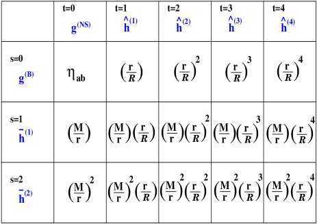
FIG. 1.: An illustration of the matching scheme for a single body moving in a general vacuum exterior spacetime $g_{ab}^{(B)}$. The tensors $g_{ab}^{({\rm NS})}$, ${\hat{h}}_{ab}^{(1)}$, ${\hat{h}}_{ab}^{(2)},\ldots$ when expanded in power series in $M/r$ yield the columns in this diagram. Similarly, the the tensors $g_{ab}^{(B)}$, ${\bar{h}}_{ab}^{(1)}$, ${\bar{h}}_{ab}^{(2)}$ when expanded in power series in $r/{\cal R}$ and when acted on by the pullback map (59) yield the rows. The matching procedure consists of demanding consistency between the two sets of expansions at each order $(s,t)$ in the double expansion, wherein the metric perturbations scale as $(M/r)^{s}(r/{\cal R})^{t}$. In the external spacetime, the metric perturbation ${\bar{h}}_{ab}^{(1)}$ is determined by the $(s,t)=(1,0)$ matching, and ${\bar{h}}_{ab}^{(2)}$ by the $(s,t)=(2,0)$ and $(2,1)$ matchings. In the internal scheme, the metric perturbation ${\hat{h}}_{ab}^{(1)}$ vanishes identically, ${\hat{h}}_{ab}^{(2)}$ is determined by the $(s,t)=(0,2)$ matching, ${\hat{h}}_{ab}^{(3)}$ is determined by the $(0,3)$ and $(1,3)$ matchings, and ${\hat{h}}_{ab}^{(4)}$ by the $(0,4)$, $(1,4)$ and $(2,4)$ matchings.

Turn next to the perturbations ${\hat{h}}_{ab}^{(3)}$ and ${\hat{h}}_{ab}^{(4)}$. The free parameters in these perturbations are the quantities $b_{Jm}^{(3)}$, $d_{Jm}^{(3)}$, $b_{Jm}^{(4)}$ and $d_{Jm}^{(4)}$ in Eqs. (121) – (122), and are determined by the matching scheme. As explained in Sec. IV A above, the values of these parameters will not affect the change in central density of the neutron star and thus are unimportant for our purposes. For completeness we briefly mention how these parameters are determined. First, since ${\hat{h}}_{ab}^{(3)}$ diverges like $r^{3}$ at large $r$, it contains only $J=3$ and $J=2$ pieces. The $J=3$ piece is determined by the $(s,t)=(0,3)$ matching, and depends linearly on the spatial derivatives of the electric and magnetic parts of the Weyl tensor of the background spacetime $g_{ab}^{(B)}$, evaluated on the geodesic. The $J=2$ piece is determined by the $(1,3)$ matching, and depends on the first order perturbation ${\bar{h}}_{ab}^{(1)}$ in the external spacetime as well as on the background metric $g_{ab}^{(B)}$. Specifically, ${\bar{h}}_{ab}^{(1)}$ is first determined by the $(1,0)$ matching [27], and from this one can calculate the $(1,3)$ element of the matrix in Fig. 1, and hence infer the $J=2$ piece of ${\hat{h}}_{ab}^{(3)}$. Note that $h_{ab}^{(3)}$ thus depends on the geometry of $g_{ab}^{(B)}$ not just in a neighborhood of the geodesic, but also non-locally [56]. In a similar way ${\hat{h}}_{ab}^{(4)}$ contains pieces with $0\leq J\leq 4$ in the term ${}^{0}h_{ab}^{(4)}$ in Eq. (121) which are independent of the $t=4$ matchings, and pieces with $2\leq J\leq 4$ in the second term in Eq. (121) which are determined by the $t=4$ matchings. These additional $2\leq J\leq 4$ pieces depend on ${\bar{h}}_{ab}^{(1)}$ and ${\bar{h}}_{ab}^{(2)}$ in addition to $g_{ab}^{(B)}$ and are determined by the $(0,4)$, $(1,4)$ and $(2,4)$ matchings.

Returning to the $O(\varepsilon^{2})$ perturbation, it follows from the arguments of Sec. IV A that the leading order change (128) in central density depends quadratically on ${\hat{h}}_{ab}^{(2)}$, and hence quadratically on ${\cal E}_{ij}$ and ${\cal B}_{ij}$, the curvatures of the external background spacetime $g_{ab}^{(B)}$ evaluated on the worldline. Furthermore, since all the relevant equations are elliptic, the dependence of $\delta\rho_{c}$ on ${\cal E}_{ij}$ and ${\cal B}_{ij}$ is local in time. Hence, invariance under rotations yields

$${\delta\rho_{c}(t)\over\rho_{c}}=c_{1}{\cal E}_{ij}(t){\cal E}^{ij}(t)+c_{2}{\cal B}_{ij}(t){\cal B}^{ij}(t)+O({\cal R}^{-5}),$$ (130)

where $c_{1}$ and $c_{2}$ are constants of dimension (length)^-4 that depend on $M$, $R$ and on the equation of state. (A cross term between the ${\cal E}_{ij}$ and ${\cal B}_{ij}$ fields is forbidden by parity arguments.)

Thus, Eqs. (41) – (43) have the same structure as their Newtonian and post-Newtonian counterparts. Equations (41), (42) together with Eqs. (47), (48) describe distortions of the star induced by the external tidal fields, where there is no change in the star’s central density and no excitation of the star’s $J=m=0$ modes. Equation (43) describes the second-order effect of the leading-order tidal field ${\hat{h}}_{ab}^{(2)}$ on the star’s structure. Exactly as in Newtonian gravity, it is this second-order effect of the leading-order tidal field that excites the spherically symmetric, radial modes of the star and changes the star’s central density and angle-averaged radius.

It is possible to understand this result in a fairly simple, intuitive way. Consider first a weakly self-gravitating body in an external gravitational field in the tidal limit $R\ll{\cal R}$. Simply analyzing the dynamics of the test body using Fermi-normal coordinates (9) allows one to immediately conclude that the effect of the external field on the body’s internal dynamics must scale as ${\cal R}^{-2}$; this is just the equivalence principle. The fact that there is no spherically symmetric interaction at this order (that is, that the interaction can be called a “tidal” interaction) follows from algebraic properties of general relativity – the relativistic generalization of the familiar fact that the trace of the Newtonian tidal force tensor $\partial^{2}\Phi/\partial x^{i}\partial x^{j}$ vanishes. As a consequence of this vanishing of the spherically symmetric interaction, all radial crushing or anti-crushing forces must scale as ${\cal R}^{-4}$. At first sight the above argument does not apply to a strongly self-gravitating body. However, the essence of the argument can be carried through. What is relevant for determining the interaction between the body and the external field are Einstein’s equations in the matching region $R\ll r\ll{\cal R}$ (the body’s “local asymptotic rest frame” [58]). The asymptotic value of the external spacetime’s curvature tensors in this region (which is the region $r\to 0$ as seen in the external spacetime) act as a source for the interaction, and their scaling ($\propto{\cal R}^{-2}$) and algebraic properties determine the nature of the interaction in the same way as for a weakly self-gravitating body.

To conclude, we have shown that, just as in Newtonian gravity, the leading order change in the central density of a fully relativistic spherical star freely falling in an external vacuum gravitational field is given by the star’s second-order response to the leading order, external tidal field.

V MODIFIED MATCHED ASYMPTOTIC EXPANSION METHOD APPLICABLE TO NEUTRON STARS IN A BINARY

The analysis of Secs. II – IV assumes that the spacetime outside the body is vacuum. This assumption entered in the equation of motion (53) satisfied by the metric perturbation ${\bar{h}}_{ab}^{(1)}$, which is used to derive the fact that the star travels along a geodesic of the background metric $g_{ab}^{(B)}$ to leading order [cf. Eq. (60) above]. It is possible to modify the analysis of Secs. II – IV to accommodate two freely falling bodies, for examples two neutron stars moving in the vicinity of a supermassive black hole. In this case the metric perturbation ${\bar{h}}_{ab}^{(1)}$ describes the linearized gravitational interactions of the two neutron stars, and one must solve simultaneously for the external metric perturbations, for two sets of internal metric perturbations, one for each star, and likewise for two sets of embedding functions. The scheme allows one to derive, for example, the equations of motion of two “point particles” interacting via their linearized gravitational fields.

Such a calculational scheme is applicable in principle to an isolated neutron star binary, but is poorly adapted to that situation. Since the background metric $g_{ab}^{(B)}$ is a flat Minkowski metric in this context, the calculations of Secs. II – IV of the leading order change in central density are not applicable. Moreover, to achieve our goal of determining the scaling of the change in central density with the parameters $\epsilon$ and $\alpha$ discussed in Sec. I A, one should describe the gravitational interactions of the two neutron stars not by metric perturbations ${\bar{h}}_{ab}^{(1)}$ and ${\bar{h}}_{ab}^{(2)}$, but rather in terms of a post-Newtonian expansion. For these reasons, in this section we outline a modified, matched asymptotic expansion calculational method in which metric perturbations in an internal scheme are matched onto post-Newtonian quantities in an external scheme. The modified method will allow us to calculate the change in central density for neutron stars in a binary.

As in Sec. II above, the method consists of an internal scheme, an external scheme, and a matching scheme. A key difference is that there are two sets of internal schemes and two sets of matchings, one for each star, all of which must be solved self-consistently.

A The external scheme

Let $M^{(B)}$ be the external manifold in which the neutron stars move. The gravitational field is described in the external scheme by the standard post-Newtonian expansion in vacuum. Thus the zeroth order, background solution is just a Newtonian spacetime, instead of the vacuum Lorentzian metric $g_{ab}^{(B)}$ we had previously. The metric perturbations ${\bar{h}}_{ab}^{(s)}$ are replaced by post-Newtonian fields, post-post-Newtonian fields, etc [59].

Now, any Newtonian spacetime can be characterized by a lengthscale ${\cal L}$ and a massscale $M$, such that the typical value of the Newtonian potential is $\sim M/{\cal L}$ and such that the local radius of curvature ${\cal R}_{c}$ is given by ${\cal R}_{c}^{-2}\sim M/{\cal L}^{3}$. In our example of a neutron star binary, ${\cal L}$ will be just the orbital separation $L$. The post-$s/2$-Newtonian fields, for $s=0,1,2\ldots$, scale as $M^{s/2}$, but have no definite scaling with respect to ${\cal L}$. This is analogous to the behavior of the expansion (52). As is well known, the post-Newtonian fields corresponding to odd values of $s$ vanish identically for $s=1,3$ and start at $s=5$.

In a suitable coordinate system ${\bar{x}}^{\alpha}=({\bar{t}},{\bar{x}}^{i})$, the metric up to post-1-Newtonian order can be written in the standard form [61]

$$ds^{2} = -\big{[}1+2\varepsilon^{2}\Phi({\bar{x}}^{i},\varepsilon{\bar{t}})+2\varepsilon^{4}\Phi({\bar{x}}^{i},\varepsilon{\bar{t}})^{2}+2\varepsilon^{4}\Psi({\bar{x}}^{i},\varepsilon{\bar{t}})$$ (133)

$$+O(\varepsilon^{6})\big{]}d{\bar{t}}^{2}+2d{\bar{x}}^{i}d{\bar{t}}\left[\varepsilon^{3}W_{i}({\bar{x}}^{i},\varepsilon{\bar{t}})+O(\varepsilon^{5})\right]$$

$$+d{\bar{x}}^{i}d{\bar{x}}^{j}\left[\delta_{ij}-2\varepsilon^{2}\Phi({\bar{x}}^{i},\varepsilon{\bar{t}})\delta_{ij}+O(\varepsilon^{4})\right],$$

where $\varepsilon\ \propto\ \sqrt{M}$ is a formal expansion parameter. Equivalently, by making a gauge change ${\bar{t}}\to{\bar{t}}/\varepsilon$, the metric can be written as

$$ds^{2} = -{1\over\varepsilon^{2}}\Big{[}1+2\varepsilon^{2}\Phi({\bar{x}}^{i},{\bar{t}})+2\varepsilon^{4}\Phi({\bar{x}}^{i},{\bar{t}})^{2}+2\varepsilon^{4}\Psi({\bar{x}}^{i},{\bar{t}})$$ (136)

$$+O(\varepsilon^{6})\Big{]}d{\bar{t}}^{2}+2d{\bar{x}}^{i}d{\bar{t}}\left[\varepsilon^{2}W_{i}({\bar{x}}^{i},{\bar{t}})+O(\varepsilon^{4})\right]$$

$$+d{\bar{x}}^{i}d{\bar{x}}^{j}\left[\delta_{ij}-2\varepsilon^{2}\Phi({\bar{x}}^{i},{\bar{t}})\delta_{ij}+O(\varepsilon^{4})\right].$$

In vacuum one can pick a gauge in which the potentials $\Phi$, $\Psi$ and $W_{i}$ obey the equations [61]

$$\nabla^{2}\Phi=\nabla^{2}W_{i}=\nabla^{2}\Psi+{\ddot{\Phi}}=0,$$ (137)

where $\nabla^{2}$ is the Laplacian of flat space.

The post-Newtonian expansion can also be described in a coordinate-free way [62]. Let $g^{ab}(\varepsilon)$ be a one parameter family of vacuum metrics which are $C^{2}$ in $\varepsilon^{2}$ in a neighborhood of $\varepsilon=0$, such that the limit $\varepsilon\to 0$ of $g^{ab}(\varepsilon)$ exists and is of signature $(0,+,+,+)$. [The formula (136) gives an approximate version of such a family]. Then there exist tensor fields $h^{ab}$, $t_{a}$ and a connection $D_{a}$ such that

$$g^{ab}(\varepsilon) = h^{ab}+O(\varepsilon^{2})$$ (138)

$$\varepsilon^{2}g_{ab}(\varepsilon) = -t_{a}t_{b}+O(\varepsilon^{2})$$ (139)

$$\nabla_{a}(\varepsilon) = D_{a}+O(\varepsilon^{2}).$$ (140)

The quantities $D_{a}$, $h^{ab}$ and $t_{a}$ comprise a Newtonian spacetime. In Newtonian or “inertial” coordinate systems $({\bar{x}}^{i},{\bar{t}})$, these quantities are given by $t_{a}=(d{\bar{t}})_{a}$, $h^{ab}=\delta_{ij}(\partial/\partial{\bar{x}}^{i})^{a}(\partial/\partial{\bar{x}}^{j})^{b}$, and $D_{a}$ is given in terms of the Newtonian potential $\Phi$ by the only non-vanishing connection coefficient being $\Gamma^{i}_{tt}=\Phi_{,i}$. The Newtonian fields satisfy the additional relations

$$D_{a}t_{b}=D_{a}h^{bc}=h^{ab}t_{b}=h^{a[b}R^{c]}_{\ (de)a}=0,$$ (141)

where $R^{a}_{\ bcd}$ is the curvature of the connection $D_{a}$. The last of the relations (141) is just the the limit $\varepsilon\to 0$ of the identity $g^{a[b}(\varepsilon)R^{c]}_{\ (de)a}(\varepsilon)=0$. The higher order correction terms in Eqs. (138) – (140) of order $O(\varepsilon^{s})$ collectively describe the post-$s/2$-Newtonian fields; we shall not need the precise forms of these fields here [64].

B The internal scheme

The internal scheme is very similar to that described in Sec. II C 1 above. The interior metric still is given by Eq. (17), however now each term $\varepsilon^{t}{\hat{h}}_{ab}^{(t)}$ in that expansion scales as ${\cal L}^{-t/2}$ rather than ${\cal R}^{-t}$, and has no definite scaling with respect to $M$. The reason that we need to include half-integral powers of $1/{\cal L}$ is that time derivatives will scale like ${\cal L}^{-3/2}$.

The equations of motion (41) – (51) are modified by the following two considerations. First, time-derivatives now scale as $\varepsilon^{3}$ rather than $\varepsilon$, which modifies the form of the perturbation analysis. Hence, a time derivative of the field ${\hat{h}}_{ab}^{(t)}$ will enter as a source term in the equation for the field ${\hat{h}}_{ab}^{(t+3)}$. The perturbations ${\hat{h}}_{ab}^{(t)}$ with $t$ odd are due entirely to such time-derivative source terms. Since it turns out that the first non-vanishing perturbation occurs at $O(\varepsilon^{6})$, the first non-vanishing ${\hat{h}}_{ab}^{(t)}$ with $t$ odd occurs for $t=9$. The second consideration is that we need now to consider the perturbations up to order $t=12$ instead of up to order $t=4$. This is not as complex as it seems since it suffices to consider even values of $t$ until $t=9$. In addition, as already mentioned the first non-vanishing perturbation is ${\hat{h}}_{ab}^{(6)}$.

The structure of the resulting equations of motion is closely analogous to that of Eqs. (41) – (51), and the general solutions follow the same pattern as the solutions (115), (116) and (119) – (122). As before, the crucial aspect of the solutions that we shall use is that the first non-vanishing perturbation in the $J=0$ sector cannot arise directly from matching to the external scheme, but must arise from a source term that is quadratic in a lower order field.

In what follows, we neglect entirely odd values of $t$. This is justified since, just as in Sec. IV B above, all time-derivative-generated terms have no $J=0$ parts and will not contribute to the leading order change in central density.

C The matching scheme

The construction of the matching scheme parallels that given in Sec. II C 3 above. One needs to specify an embedding

$$\varphi:\ M^{({\rm NS})}\to M^{({\rm B})},$$ (142)

of the neutron star spacetime into the external spacetime, i.e., a mapping between the asymptotically Lorentzian coordinates $x^{\alpha}$ of $M^{({\rm NS})}$ and the coordinates ${\bar{x}}^{\alpha}$ of $M^{({\rm B})}$. We can write this mapping as [compare Eq. (59) above]

$${\bar{x}}^{\alpha} = {\bar{x}}^{\alpha}(t,x^{i})$$ (143)

$$= \sum_{p=0}\,\left({M\over{\cal L}}\right)^{p/2}\,\sum_{r=0}\,\sum_{I_{r}}\ \ {}^{(r,p)}{\cal F}^{\alpha}_{I_{r}}(t)\,x^{I_{r}},$$ (144)

where $I_{r}$ denotes the multi-index $(i_{1},\ldots,i_{r})$ and $x^{I_{r}}\equiv x^{i_{1}}x^{i_{2}}\ldots x^{i_{r}}$. Equation (59) is a Taylor expansion of $\varphi$ in terms both of the spatial coordinates $x^{i}$ at each fixed $t$, and also in terms of the parameter $\sqrt{M/{\cal L}}$. The terms with $p$ odd are vanishing for $p=1,3$; the first non-vanishing terms with $p$ odd start at $p=5$. Thus, the worldline of the center of the neutron star gets mapped onto the worldline

$${\bar{x}}^{\alpha}(t)={}^{(0,0)}{\cal F}^{\alpha}(t)+{M\over{\cal L}}{}^{(0,2)}{\cal F}^{\alpha}(t)+O[(M/{\cal L})^{2}].$$ (145)

The matching procedure described below can be used to show that the first term in Eq. (145) represents a worldline satisfying Newtonian equations of motion, that the second term is the first post-Newtonian, point mass correction, etc.

Next, from the interior metric $g_{ab}^{({\rm INTERIOR})}$ on $M^{({\rm NS})}$ one construct the metric

$${\bar{g}}_{ab}=\left(\varphi^{-1}\right)_{*}\chi_{*}g_{ab}^{({\rm INTERIOR})}$$ (146)

on $M^{(B)}$. Here $\chi:M^{({\rm NS})}\to M^{({\rm NS})}$ is the mapping defined after Eq. (27) above, with the parameter $\varepsilon$ chosen to have the value $\sqrt{M}$. The metric $\chi_{*}g_{ab}^{({\rm INTERIOR})}$ will have a dependence on $\sqrt{M}$ like that of the metric (136) has on $\varepsilon$. Now perform a double power series expansion of the metric ${\bar{g}}_{ab}$, its inverse ${\bar{g}}^{ab}$ and its associated connection ${\bar{\nabla}}_{a}$ in terms of the parameters $M/r$ and $r/{\cal L}$, as in Eq. (55) above. These double power series expansion must be consistent, order by order, with expansions in powers of $r/{\cal L}$ of the post-$s/2$-Newtonian fields for $s=0,2,4,5,\ldots$ of the external scheme. As before, demanding such consistency determines both the embedding free functions and the appropriate solutions in the internal and external schemes, up to some gauge freedom.

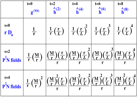
FIG. 2.: An illustration of the matching scheme for a body moving in a spacetime described by a post-Newtonian approximation. In the external spacetime, the post-$s/2$-Newtonian fields for $s=0,2,4$, when expanded in power series in $r/{\cal L}$, yield the rows in this diagram. The sum of $g_{ab}^{({\rm NS})}$, ${\hat{h}}_{ab}^{(1)}$, ${\hat{h}}_{ab}^{(2)},\ldots$ when acted on by the pullback map (146) yields a tensor field ${\bar{g}}_{ab}(M)$ on the external spacetime. When one considers the triple $\left(M\,{\bar{g}}_{ab}(M),{\bar{g}}^{ab}(M),{\bar{\nabla}}_{a}(M)\right)$, and expands this triple order by order in $M$, one obtains at $O(M^{s/2})$ the post-$s/2$-Newtonian fields, for $s=0,2,4,5\ldots$. The expansions in powers of $r/{\cal L}$ of these fields must agree with those of the external spacetime post-Newtonian fields. In the internal scheme, the metric perturbations ${\hat{h}}_{ab}^{(2)}$ and ${\hat{h}}_{ab}^{(4)}$ vanish identically, and ${\hat{h}}_{ab}^{(6)}$ is determined by the $(s,t)=(0,6)$ matching. The first change in central density occurs in ${\hat{h}}_{ab}^{(12)}$.

Consider for example the case $s=0$, which is just the matching onto a Newtonian spacetime. The limit $M\to 0$ of the fields ${\bar{g}}_{ab}$, ${\bar{g}}^{ab}$ and ${\bar{\nabla}}_{a}$ yields yields Newtonian fields ${\bar{h}}^{ab}$, ${\bar{t}}_{a}$ and ${\bar{D}}_{a}$, cf. Eqs. (138) – (140) above. The expansion in powers of $r/{\cal L}$ of these fields must agree, order by order, with the expansions in powers of $r/{\cal L}$ of the Newtonian fields $h^{ab}$, $t_{a}$, and $D_{a}$ of the external scheme. If we choose the coordinate system (13) in the internal scheme and a Newtonian or inertial coordinate system $({\bar{x}}^{i},{\bar{t}})$ in the internal scheme, then the fields $h^{ab}$, ${\bar{h}}^{ab}$ and $t_{a}$, ${\bar{t}}_{a}$ will coincide to all orders in $r/{\cal L}$ if we choose the embedding (142) to be of the form ${\bar{t}}(x^{j},t)=t$, ${\bar{x}}^{i}(x^{j},t)=x^{i}+f^{i}(t)$. Then one just has to match the Newtonian potentials order by order in $r/{\cal L}$.

This matching to zeroth order in $r/{\cal L}$ [i.e., the $(s,t)=(0,0)$ matching] yields the usual Newtonian point-mass equations of motion. Hence, when one solves for the embedding functions of both stars and for the interior and exterior gravitational fields up to order $(s,t)=(0,0)$, the result is two static spherical neutron stars moving along their Newtonian orbits. This then serves as the starting point for calculating higher order perturbations.

This matching procedure is illustrated schematically in Fig. 2. Our arguments below will be independent of the details of the post-Newtonian and post-post-Newtonian matchings, so we do not need to describe those here.

D Change in central density

The leading order change in central density $\delta\rho_{c}$ of a neutron star in a binary can now be deduced by arguments analogous to those given in Sec. IV B above. First, in the internal scheme we need consider only even values of $t$, as explained in Sec. V B. Next, consider the perturbations ${\hat{h}}_{ab}^{(2)}$ and ${\hat{h}}_{ab}^{(4)}$. If these perturbations were to be non-zero (or not pure gauge), then they would need to diverge at large $r$ like $r^{J}$ for some $J\geq 2$, from the analysis in Sec. III. But from Fig. 2, ${\hat{h}}_{ab}^{(2)}\sim{\rm const}$ and ${\hat{h}}_{ab}^{(4)}\ \propto\ r$ at large $r$. Hence the first non-vanishing perturbation is ${\hat{h}}_{ab}^{(6)}$, which is purely $J=2$. Note that this perturbation is determined entirely by the exterior Newtonian fields from the $(s,t)=(0,6)$ matching.

Since the first non-vanishing perturbation is ${\hat{h}}_{ab}^{(6)}$, the first change in central density must scale as $({\hat{h}}_{ab}^{(6)})^{2}$ by the same arguments as before, so we must have

$${\delta\rho_{c}\over\rho_{c}}\propto{1\over{\cal L}^{6}}$$ (147)

at large ${\cal L}$. The constant of proportionality in Eq. (147) must have dimensions of $({\rm length})^{6}$, and the only relevant dimensionful parameters are the mass $M$ of the star and its radius $R$. We can therefore write

$${\delta\rho_{c}\over\rho_{c}}=F[M/R]\left({R\over{\cal L}}\right)^{6}=F(\epsilon)\alpha^{6}+O(\alpha^{7}),$$ (148)

where $F$ is a dimensionless function of a dimensionless variable, and we have used the dimensionless variables $\alpha\equiv R/L$ and $\epsilon\equiv M/R$ discussed in the Introduction. The function $F$ will depend on the equation of state.

VI DISCUSSION AND CONCLUSIONS

As discussed in the Introduction, the result (148) is in disagreement with Refs. [1, 2] in the regime $\alpha\ll 1$ where there should be agreement, since the scaling found in the numerical simulations is $\delta\rho_{c}/\rho_{c}\propto\alpha^{2}$ as $\alpha\to 0$. This disagreement in scaling at large orbital separations is strong evidence that the star crushing effect seen in Refs. [1, 2] is not physical.

In addition, at the location of the instability seen by Wilson et. al. , the dimensionless parameter $\alpha^{6}$ is of order $10^{-4}$, so one might expect the perturbative result (148) to be a good approximation. For $F(\epsilon)$ of order unity, the fractional change in central density (148) at this location is $\sim 1000$ times smaller than that seen in the numerical simulations [1, 2].

The analysis of this paper does not determine the sign of the function $F(\varepsilon)$. However, we can make the following argument. Let us expand this function as a power series, which yields an expression of the form

$${\delta\rho_{c}\over\rho_{c}}=F_{0}\alpha^{6}\left[1+F_{1}\epsilon+F_{2}\epsilon^{2}+\ldots\right],$$ (149)

for some constant coefficients $F_{0}$, $F_{1}$, $F_{2}$ etc. Now, it is known from Lai’s Newtonian analysis that the coefficient $F_{0}$ is negative [7, 65]. Therefore, unless the dimensionless coefficients $F_{1}$, $F_{2}$ etc are negative and large ($\sim-7$ for $F_{1}$), which seems unlikely, the change in central density due to the tidal interaction will be negative. Thus, the stars angle-averaged radius will increase and the star will be more stable and not less stable to radial collapse.

Note that our analysis assumes that the neutron stars are not spinning in their local rest frames, although the dragging of inertial frames means that they will spin slightly with respect to distant stars; this effect is incorporated in the choice of Fermi-normal coordinates in Eq. (9).

Note also that our analysis assumes that the external tidal fields are slowly varying compared to the dynamical timescales of the neutron star, so that the stellar modes adiabatically follow their driving forces. This follows from the assumption $\alpha\ll 1$ underlying the perturbation expansion. Clearly this adiabatic approximation breaks down at $\alpha\sim 1$. However, one can ask how well we might expect the adiabatic approximation to be working at the location of the instability. For the neutron star $f$-modes and $p$-modes, the idealization is a good approximation: From the point of view of the companion star, the timescale over which the external tidal fields is varying is ${\cal T}\sim\sqrt{L^{3}/M}$. This timescale is long compared to the internal dynamical time of the neutron star (the characteristic timescale of the $f$-modes) $\sim\sqrt{R^{3}/M}$. Hence, these modes will equilibrate rapidly in response to the tidal perturbations and the approximation is fairly good. The $g$-modes of the neutron star on the other hand have frequencies $\ll\sqrt{M/R^{3}}$ and are resonantly excited [20, 22] in the Newtonian approximation near the end of the inspiral; for these modes the approximation is inappropriate. This is a limitation of the applicability of our analysis. However, it seems unlikely that resonant $g$-mode excitations could be responsible for the star crushing effect seen in the Wilson-Mathews-Marronetti simulations, since the predicted amplitudes of excitation in the Newtonian approximation are fairly small [20, 22].

Finally, consider the implications of our result for the gravitational wave signature of the inspiral. Previous analyses [17, 18, 7, 19] have shown that to Newtonian order, the effect of the finite size of the neutron stars on the gravitational waveform is small, and in fact is negligible for the purposes of signal detection. For the initial LIGO interferometers, $\sim 95\%$ of the signal-to-noise ratio will have been accumulated before the gravitational wave frequency reaches $400\,{\rm Hz}$ [see, e.g., Eq. (2.23) of Ref. [66]]. The total accumulated phase error in the signal predicted by Newtonian tidal interactions by $400\,{\rm Hz}$ is $\ll 1$; see Eq. (7.5) of Ref. [7] and Ref. [19]. We have shown using a fully relativistic treatment of tidal interactions that, as one would expect, the Newtonian predictions for tidal interactions are valid except for correction terms of order $M/R$ and $M/L$, that is, fractional corrections $\lesssim 1$. Therefore, the effects of tidal interactions and of the finite size of the neutron stars will be unimportant for signal detection.

As this paper was being completed, we learned of a similar analysis by Thorne [58]. Thorne shows that the change in central density is $\propto\alpha^{6}$, but also that it is always negative, stabilizing the neutron star.

TABLE I.: A summary of the orders at which various physical effects occur. The parameter $\alpha$ is the tidal expansion parameter (stellar radius)/(orbital separation), and $\epsilon$ is the strength of internal gravity in each star, $\epsilon=$(stellar mass)/(stellar radius). A perturbation to the orbital motion is said to scale as $\alpha^{n}\epsilon^{m}$ if the ratio of the perturbing force to the Newtonian orbital force is of this order. Similarly, the distortion of each star is said to be of order $\alpha^{n}\epsilon^{m}$ if the dimensionless measure of distortion $(I_{xx}-I_{yy})/I_{xx}$ is of this order. Note that to post-1-Newtonian order, all the physical effects scale the same way with $\alpha$ as their Newtonian counterparts. The pattern for the stellar modes is repeated at all higher orders in $\epsilon$. The entries in the orbital motion columns can be deduced from the entries in the stellar modes columns; if $\delta{\cal E}$ is the energy transferred between the stellar modes and the orbital motion, then the fractional change in the orbital motion is $\sim L\delta{\cal E}/M^{2}$, while the fractional distortion of the star is $\sim R\delta{\cal E}/M^{2}$, one power of $\alpha$ smaller.

	Newtonian : $O(\epsilon^{0})$			$O(\epsilon)$
Tidal order	Orbital motion	Stellar modes		Orbital  motion	Stellar modes
$O(\alpha^{0})$	$\uparrow$	$\uparrow$		Newtonian orbit	$\uparrow$
$O(\alpha^{1})$	$|$	static spherical star		$\uparrow$	static spherical star
$O(\alpha^{2})$	No change in orbit	$\downarrow$		post-1-Newtonian	$\downarrow$
$O(\alpha^{3})$	$|$	$\uparrow$		point particle orbit	$\uparrow$
$O(\alpha^{4})$	$\downarrow$	tidal deformation		$\downarrow$	post-1 deformation
$O(\alpha^{5})$	$\uparrow$	$\downarrow$		$\uparrow$	$\downarrow$
$O(\alpha^{6})$	Orbit responds	$\uparrow$		orbit modified	$\uparrow$
$O(\alpha^{7})$	to tidal coupling	first change		$|$	post-1 correction to
$O(\alpha^{7})$	$|$	in central density		$|$	change in central density
$O(\alpha^{8})$	$|$	$|$		$|$	$|$