Gravitational waves from inspiraling compact binaries:
Second post-Newtonian waveforms as search templates

Abstract

We ascertain the effectiveness of the second post-Newtonian approximation to the gravitational waves emitted during the adiabatic inspiral of a compact binary system as templates for signal searches with kilometer-scale interferometric detectors. The reference signal is obtained by solving the Teukolsky equation for a small mass moving on a circular orbit around a large nonrotating black hole. Fitting factors computed from this signal and these templates, for various types of binary systems, are all above the 90% mark. According to Apostolatos’ criterion, second post-Newtonian waveforms should make acceptably effective search templates.

I Introduction

The current construction of kilometer-scale interferometric gravitational-wave detectors, such as the American LIGO (Laser Interferometer Gravitational-wave Observatory [1]) and the French-Italian VIRGO [2], has motivated a lot of recent work on data analysis tools to search and measure the expected gravitational-wave signals [3]. Thus far, the mostly studied waves have been those generated by the adiabatic inspiral of a compact binary system, composed of neutron stars and/or black holes [4]. Because of their reliably large event rate [5, 6, 7], these waves are currently believed to be the most promising for detection by LIGO/VIRGO. And because their waveforms can be accurately predicted, searching and measuring these waves will be best accomplished with the well-known technique of matched filtering [8]. In this paper we focus on certain issues related to the search of gravitational waves from inspiraling compact binaries.

The method of matched filtering [8] relies on the fact that an accurate model can be constructed for the expected signal. The model (usually called the template) depends on various parameters, such as the signal’s time of arrival, its initial phase, the masses of the companions, their spin angular momenta, and others. The template is cross-correlated with the detector output, and the parameters are varied until the largest correlation is obtained. If the maximum correlation (usually called the signal-to-noise ratio) is larger than a specified threshold value, then a signal is concluded to be present.

A large effort is currently underway to calculate inspiraling binary waveforms to high order in a post-Newtonian approximation [9, 10]. This approach is based on the assumption that the orbital motion is sufficiently slow that the waves can be expressed as a power series in $v/c$, the ratio of the orbital velocity to the speed of light. Because the series converges very slowly, if at all, a large number of terms are required [11, 12]. Thus far, the waveforms have been computed to order $(v/c)^{5}$ (2.5 post-Newtonian, or 2.5PN, order) beyond the leading-order, quadrupole-formula expressions [10].

Central to the theory of matched filtering is Wiener’s theorem [8], which states that the expectation value of the correlation is maximized when the template parameters match those of the actual signal. For the theorem to apply, however, the functional form of the template must be the same as that of the signal, so that template and signal are allowed to disagree only in the value of their parameters. In view of the fact that the signal is governed by the exact laws of general relativity, while the template necessarily constitutes an approximation, we must expect that the actual signal-to-noise ratio will be somewhat less than the maximum allowed by Wiener’s theorem [13]. We must also expect that the value of the template parameters which maximize the correlation will not precisely match the value of the source parameters.

Apostolatos [14] has introduced the fitting factor (FF) as a measure of template imperfection. The fitting factor is the ratio of the actual signal-to-noise ratio, obtained with the imperfect template, to the signal-to-noise ratio that would be obtained if a perfect template were available [13]. A fitting factor of unity means that the template is a very accurate representation of the signal (a perfect template). A value less than unity means that the template reproduces the signal only imperfectly. The loss in event rate due to template imperfection is given by $1-\mbox{FF}^{3}$ [14].

The fitting factor is computed as follows [14]. Let $s(t)$ be the actual signal, and let $h(t;\mathchoice{{\hbox{\boldmath$\displaystyle\theta$}}}{{\hbox{\boldmath$\textstyle\theta$}}}{{\hbox{\boldmath$\scriptstyle\theta$}}}{{\hbox{\boldmath$\scriptscriptstyle\theta$}}})$ be the templates, with the vector $\textstyle\theta$ representing the parameters. We denote the Fourier transforms of these functions by $\tilde{s}(f)$ and $\tilde{h}(f;\mathchoice{{\hbox{\boldmath$\displaystyle\theta$}}}{{\hbox{\boldmath$\textstyle\theta$}}}{{\hbox{\boldmath$\scriptstyle\theta$}}}{{\hbox{\boldmath$\scriptscriptstyle\theta$}}})$, respectively, where $\tilde{a}(f)=\int a(t)e^{2\pi ift}\,dt$ for any function $a(t)$. We define the ambiguity function ${\cal A}(\mathchoice{{\hbox{\boldmath$\displaystyle\theta$}}}{{\hbox{\boldmath$\textstyle\theta$}}}{{\hbox{\boldmath$\scriptstyle\theta$}}}{{\hbox{\boldmath$\scriptscriptstyle\theta$}}})$ by

$${\cal A}(\mathchoice{{\hbox{\boldmath$\displaystyle\theta$}}}{{\hbox{\boldmath$\textstyle\theta$}}}{{\hbox{\boldmath$\scriptstyle\theta$}}}{{\hbox{\boldmath$\scriptscriptstyle\theta$}}})=\frac{(s|h)}{\sqrt{(s|s)(h|h)}},$$ (1)

where, for any functions $a(t)$, $b(t)$,

$$(a|b)=2\int_{0}^{\infty}\frac{\bar{\tilde{a}}(f)\tilde{b}(f)+\tilde{a}(f)\bar{\tilde{b}}(f)}{S_{n}(f)}\,df.$$ (2)

Here, an overbar indicates complex conjugation, and $S_{n}(f)$ is the (one-sided) spectral density of the detector noise. For interferometric detectors of the advanced-LIGO type, it is appropriate [15] to set $S_{n}(f)=S_{0}[(f_{\rm min}/f)^{4}+2+2(f/f_{\rm min})^{2}]$ for $f>10\ \mbox{Hz}$, while $S_{n}(f)=\infty$ for $f>10\ \mbox{Hz}$; $S_{0}$ is a normalization constant irrelevant for our purposes, and $f_{\rm min}=70\ \mbox{Hz}$ is the frequency at which the noise is minimum. The quantity $(a|b)$ is usually interpreted as an inner product in the Hilbert space of gravitational-wave signals [15], and $\arccos{\cal A}(\mathchoice{{\hbox{\boldmath$\displaystyle\theta$}}}{{\hbox{\boldmath$\textstyle\theta$}}}{{\hbox{\boldmath$\scriptstyle\theta$}}}{{\hbox{\boldmath$\scriptscriptstyle\theta$}}})$ is the angle between the signal $s(t)$ and the template $h(t;\mathchoice{{\hbox{\boldmath$\displaystyle\theta$}}}{{\hbox{\boldmath$\textstyle\theta$}}}{{\hbox{\boldmath$\scriptstyle\theta$}}}{{\hbox{\boldmath$\scriptscriptstyle\theta$}}})$. The fitting factor is given by

$$\mbox{FF}=\max_{\mathchoice{{\hbox{\boldmath$\displaystyle\theta$}}}{{\hbox{\boldmath$\textstyle\theta$}}}{{\hbox{\boldmath$\scriptstyle\theta$}}}{{\hbox{\boldmath$\scriptscriptstyle\theta$}}}}\,{\cal A}(\mathchoice{{\hbox{\boldmath$\displaystyle\theta$}}}{{\hbox{\boldmath$\textstyle\theta$}}}{{\hbox{\boldmath$\scriptstyle\theta$}}}{{\hbox{\boldmath$\scriptscriptstyle\theta$}}}),$$ (3)

and $\arccos\mbox{FF}$ is the minimum value of this angle. Apostolatos [14] has suggested that templates for which $\mbox{FF}>90\%$ would be acceptably accurate, leading to a loss in event rate no larger than approximately 27%.

To compute the fitting factor one must first provide a reference signal $s(t)$ and a parameterized set of templates $h(t;\mathchoice{{\hbox{\boldmath$\displaystyle\theta$}}}{{\hbox{\boldmath$\textstyle\theta$}}}{{\hbox{\boldmath$\scriptstyle\theta$}}}{{\hbox{\boldmath$\scriptscriptstyle\theta$}}})$. While post-Newtonian waveforms make an obvious choice of templates, the selection of a reference signal is much more delicate, because an exact representation of the gravitational waves is not available. In all studies undertaken thus far [14, 16, 17, 18, 19, 20, 21], the reference signal was also chosen to be a post-Newtonian waveform, but one computed with more accuracy than the templates. (For example, the signal is taken to be a 2.5PN waveform, while the templates are chosen to be Newtonian, or 1PN, or 1.5PN, or 2PN waveforms.) This approach is flawed, because even a high-order post-Newtonian approximation may still be a poor representation of the true general-relativistic signal [11].

In this paper we make a different choice of reference signal which, we believe, bears a closer resemblance to the true general-relativistic signal for binary systems with small mass ratios. This signal is obtained by solving the Teukolsky equation [22] for the gravitational perturbations produced by the circular motion of a small mass around a large nonrotating black hole [23, 24]. In this approach, no assumption is made regarding the size of $v$, the orbital velocity. This is one advantage over post-Newtonian theory. However, one disadvantage is the necessary restriction to binary systems with small mass ratios.

TABLE I.: The binary systems considered in this paper are listed in the increasing order of their total mass. The individual masses $m_{1}$ and $m_{2}$, and the chirp mass ${\cal M}_{\rm actual}$ are given in solar units. The mass-ratio parameter $\eta_{\rm actual}$ is dimensionless. All quantities are defined in the text.

System	$m_{1}$	$m_{2}$	${\cal M}_{\rm actual}$	$\eta_{\rm actual}$
$1.4+1.4$	1.4	1.4	1.2188	0.2500
$0.5+5$	0.5	5.0	1.2322	0.0826
$1.4+10$	1.4	10.0	2.9943	0.1077
$10+10$	10.0	10.0	8.7055	0.2500
$4+30$	4.0	30.0	8.7340	0.1038

Our fitting factors are therefore computed by taking $s(t)$ to be derived from the equations of black-hole perturbation theory, and by taking $h(t;\mathchoice{{\hbox{\boldmath$\displaystyle\theta$}}}{{\hbox{\boldmath$\textstyle\theta$}}}{{\hbox{\boldmath$\scriptstyle\theta$}}}{{\hbox{\boldmath$\scriptscriptstyle\theta$}}})$ to be given by the so-called restricted second post-Newtonian approximation. (This terminology will be explained below; we use 2PN waveforms because the formally more accurate 2.5PN waveforms are known to be a poorer representation of the true signal [11].) We consider the binary systems listed in Table I, which consist of three low mass-ratio systems ($0.5M_{\odot}+5M_{\odot}$, $1.4M_{\odot}+10M_{\odot}$, and $4M_{\odot}+30M_{\odot}$, where $M_{\odot}$ is the solar mass) and two equal-mass systems ($1.4M_{\odot}+1.4M_{\odot}$ and $10M_{\odot}+10M_{\odot}$). Although our analysis is not expected to be valid for the equal-mass systems, we nevertheless include them as an indication of the robustness of our conclusions. For all binary systems the companions are assumed to be nonrotating.

TABLE II.: Searching perturbation-theory signals with second post-Newtonian templates. For each binary system, and for two types of signals, we list the values of ${\cal M}^{*}$, $\eta^{*}$, and $t^{*}$ corresponding to the global maximum of ${\cal A}(t^{*},{\cal M}^{*},\eta^{*})$. The fitting factor is also listed. All quantities are defined in the text. For all numbers the numerical uncertainty is $\pm 5$ in the last digit.

System	Signal	${\cal M}^{*}_{\rm max}$	$\eta^{*}_{\rm max}$	$t^{*}_{\rm max}$	FF
$1.4+1.4$	one-mode	1.0033	0.401	$0.3608\times 10^{-4}$	94.7%
$1.4+1.4$	$l\leq 3$	1.0033	0.402	$0.3562\times 10^{-4}$	93.0%
$0.5+5$	one-mode	1.0017	0.550	$0.2345\times 10^{-4}$	97.8%
$0.5+5$	$l\leq 3$	1.0017	0.550	$0.2421\times 10^{-4}$	95.2%
$1.4+10$	one-mode	1.0013	0.496	$-0.2186\times 10^{-3}$	95.5%
$1.4+10$	$l\leq 3$	1.0013	0.496	$-0.2154\times 10^{-3}$	91.4%
$10+10$	one-mode	1.0001	0.388	$-0.1197\times 10^{-3}$	98.4%
$10+10$	$l\leq 3$	1.0001	0.388	$-0.1179\times 10^{-2}$	91.7%
$4+30$	one-mode	0.9859	0.367	$-0.5256\times 10^{-2}$	95.4%
$4+30$	$l\leq 3$	0.9859	0.367	$-0.5192\times 10^{-2}$	86.6%

Our results, displayed in Table II, show that the 2PN waveforms make acceptably accurate templates, in the sense of Apostolatos’ criterion [14]: except for the large-mass system $4M_{\odot}+30M_{\odot}$, the fitting factors are all above the $90\%$ mark. This is the main conclusion of this paper. We must point out that our analysis ignores such important issues as discrete template spacing [25, 26], computing power, and spin-induced signal modulations [14, 27]. We leave such considerations for future work. Throughout the paper we work in units such that $G=c=1$.

II Reference signal

The formalism of black-hole perturbation theory [23] returns the following expression for the gravitational waves emitted by a mass $m_{1}$ in a fixed circular orbit around a nonrotating black hole of mass $m_{2}\gg m_{1}$:

$$s_{+}(t)-is_{\times}(t)\propto\sum_{l=2}^{\infty}\sum_{m=-l}^{l}A_{lm}(v)\,e^{-im\Omega t}\,\mbox{}_{-2}Y_{lm}(\theta,\phi).$$ (4)

Here, $s_{+}(t)$ and $s_{\times}(t)$ are the two fundamental polarizations of the gravitational waves, $A_{lm}(v)$ are mode amplitudes, and $\mbox{}_{-2}Y_{lm}(\theta,\phi)$ are spin-weighted spherical harmonics [28], with $\theta$ and $\phi$ the polar angles of the gravitational-wave detector. The missing normalization constant is unimportant for our purposes. In Eq. (4), the orbital velocity $v$ and the orbital angular velocity $\Omega$ are related by $v^{3}=M\Omega$, where $M=m_{1}+m_{2}$ is the total mass. The mode amplitudes $A_{lm}(v)$ must be calculated separately for each value of $v$ by numerically integrating the Teukolsky equation [24].

Equation (4) describes the waves produced by a mass moving on a fixed orbit. This expression is easily generalized to describe an adiabatic inspiral: the orbital velocity $v$ now becomes a function of time, which is determined by

$$\frac{dv}{dt}=\frac{32\mu}{5M^{2}}\,v^{9}\,\frac{P(v)}{Q(v)}.$$ (5)

Here, $\mu=m_{1}m_{2}/M$ is the reduced mass, $P(v)=(dE/dt)/(dE/dt)_{N}$ is the rate at which the gravitational waves remove orbital energy from the system, normalized to the quadrupole-formula expression $(dE/dt)_{N}=-(32/5)(\mu/M)^{2}v^{10}$, and $Q(v)=(dE/dv)/(dE/dv)_{N}=(1-6v^{2})(1-3v^{2})^{-3/2}$ gives the differential relation between orbital energy and orbital velocity, normalized to the Newtonian expression $(dE/dv)_{N}=-\mu v$. The function $P(v)$ must be computed numerically [24]. As a consequence of the time dependence of $\Omega=v^{3}/M$, the factor $\Omega t$ in Eq. (4) must be replaced by $\Phi(t)=\int^{t}\Omega(t^{\prime})\,dt^{\prime}$.

To simplify the expressions we assume that the detector is situated at $\phi=0$, so that the spherical harmonics are functions of $\theta$ only. (Because the orbit is circular, this assumption implies no loss of generality.) We also assume that the detector is oriented in such a way that it is sensitive only to the “$+$” polarization [29]. Simple manipulations, using the relation $A_{l,-m}=(-1)^{l}\bar{A}_{lm}$ [30], then bring Eq. (4) to the form

$$s(t)\propto\sum_{l=2}^{\infty}\sum_{m=1}^{l}\mbox{Re}\Bigl{[}A_{lm}(v)e^{-im\Phi(v)}\Bigr{]}\,S_{lm}(\theta),$$ (6)

where $s(t)\equiv s_{+}(t)$,

$$\Phi(v)=\frac{5M}{32\mu}\int^{v}\frac{Q(v^{\prime})}{v^{\prime 6}P(v^{\prime})}\,dv^{\prime},$$ (7)

and $S_{lm}(\theta)=\mbox{}_{-2}Y_{lm}(\theta,0)+(-1)^{l}\mbox{}_{-2}Y_{l,-m}(\theta,0)$. The relation between $t$ and $v$ is given implicitly by Eq. (5).

Equations (6) and (7) give the reference signal in the time domain. Computation of the fitting factor, however, requires an expression in the frequency domain. We must therefore Fourier transform Eq. (6), which we do in the stationary phase approximation. Skipping all intermediary steps, we find

$$\tilde{s}(f)\propto\sum_{l=2}^{\infty}\sum_{m=1}^{l}\biggl{[}\frac{Q(v)}{mv^{11}P(v)}\biggr{]}^{1/2}\,A_{lm}(v)\,e^{im\Psi(v)}\,S_{lm}(\theta),$$ (8)

where

$$\Psi(v)=\frac{5M}{32\mu}\int_{v_{0}}^{v}\frac{(v^{3}-v^{\prime 3})Q(v^{\prime})}{v^{\prime 9}P(v^{\prime})}\,dv^{\prime}.$$ (9)

In these expressions, $f$ and $v$ are related by $v=(2\pi Mf/m)^{1/3}$, and $v_{0}$ is an arbitrary constant which sets the zero of the phase function $\Psi(v)$, which must also be evaluated numerically.

In Eq. (8), the sum over $l$ must necessarily be truncated at some finite value. The dominant part of the signal comes from the $l=m=2$ mode. We shall refer to a signal containing only this mode as a one-mode signal. The second largest contribution to the signal comes from the $l=m=3$ mode, and in fact, all additional contributions can be neglected. We shall therefore truncate the sum at $l=3$, having numerically verified that additional terms are indeed irrelevant. Because $S_{33}/S_{22}=-(21/10)^{1/2}\sin\theta$, the relative importance of the $l=3$ terms is maximized when $\theta=\pi/2$. We shall therefore set $\theta$ to this value throughout the paper.

The signal must be cut off when the orbiting mass reaches the innermost stable circular orbit at $v=6^{-1/2}$. Because the $l=m=2$ mode dominates the signal, we simply let $\tilde{s}(f)=0$ when $f>(6^{3/2}\pi M)^{-1}$.

III Templates

The restricted second post-Newtonian approximation to the gravitational-wave signal is given in the frequency domain by [31]

$$\tilde{h}(f;\mathchoice{{\hbox{\boldmath$\displaystyle\theta$}}}{{\hbox{\boldmath$\textstyle\theta$}}}{{\hbox{\boldmath$\scriptstyle\theta$}}}{{\hbox{\boldmath$\scriptscriptstyle\theta$}}})\propto f^{-7/6}\,e^{i\psi(f)},$$ (10)

where $\psi(f)=2\pi ft_{c}-\phi_{c}+\phi(f)$,

$$\phi(f) = \frac{3}{128}(\pi{\cal M}f)^{-5/3}\Biggl{[}1+\frac{20}{9}\biggl{(}\frac{743}{336}+\frac{11}{4}\eta\biggr{)}\,x^{2}-16\pi x^{3}$$ (12)

$$\mbox{}+10\biggl{(}\frac{3058673}{1016064}+\frac{5429}{1008}\eta+\frac{617}{144}\eta^{2}\biggr{)}\,x^{4}\Biggr{]},$$

with $x^{3}\equiv\pi\eta^{-3/5}{\cal M}f$. Here, $\{\phi_{c},t_{c},{\cal M},\eta\}$ are the template parameters, with $\phi_{c}$ the phase at coalescence (formally $f=\infty$), $t_{c}$ the time at coalescence, $\cal M$ the chirp mass, and $\eta$ the mass-ratio parameter. The term “restricted” refers to the fact that while the phase function $\phi(f)$ is calculated to 2PN order beyond the quadrupole-formula expression, the amplitude function $f^{-7/6}$ is kept at leading order.

Because the templates do not have the same functional form as the signal, $\cal M$ and $\eta$ do not have direct physical meaning. However, if the templates were an accurate description of the waves, then the signal would be best reproduced when ${\cal M}={\cal M}_{\rm actual}$ and $\eta=\eta_{\rm actual}$, where [31]

$${\cal M}_{\rm actual}=\frac{(m_{1}m_{2})^{3/5}}{(m_{1}+m_{2})^{1/5}},\qquad\eta_{\rm actual}=\frac{m_{1}m_{2}}{(m_{1}+m_{2})^{2}},$$ (13)

with $m_{1}$ and $m_{2}$ denoting the actual masses of the companions. It is therefore convenient to introduce the rescaled parameters ${\cal M}^{*}$ and $\eta^{*}$, defined by

$${\cal M}={\cal M}^{*}{\cal M}_{\rm actual},\qquad\eta=\eta^{*}\eta_{\rm actual}.$$ (14)

It is also convenient to make the following transformations:

$$\phi_{c}=\phi_{0}+\phi^{*},\qquad t_{c}=t_{0}(1+t^{*}),$$ (15)

where

$$\phi_{0}=2\pi f_{0}t_{c}+\phi(f_{0}),\qquad t_{0}=-\frac{1}{2\pi}\,\frac{d\phi}{df}(f_{0}),$$ (16)

with $f_{0}$ an arbitrarily chosen frequency. Their purpose is to ensure that when $\phi^{*}=t^{*}=0$, then $\psi(f_{0})=d\psi/df(f_{0})=0$. These relations are analogous to those holding for $\Psi(v)$ at $v=v_{0}$ [see Eq. (9)]. We shall henceforth take $\mathchoice{{\hbox{\boldmath$\displaystyle\theta$}}}{{\hbox{\boldmath$\textstyle\theta$}}}{{\hbox{\boldmath$\scriptstyle\theta$}}}{{\hbox{\boldmath$\scriptscriptstyle\theta$}}}=(\phi^{*},t^{*},{\cal M}^{*},\eta^{*})$ to be our template parameters.

IV Computing the fitting factor

Evaluation of the ambiguity function, Eq. (1), for a given binary system and a given set of template parameters, is a straightforward numerical problem. First $A_{lm}(v)$ and $P(v)$ are computed once and for all, and tabulated for many values of the orbital velocity. Next, $\Psi(v)$ is calculated for the binary system under consideration. Combining the results and summing over the relevant modes gives $\tilde{s}(f)$, Eq. (8). On the other hand, $\tilde{h}(f;\mathchoice{{\hbox{\boldmath$\displaystyle\theta$}}}{{\hbox{\boldmath$\textstyle\theta$}}}{{\hbox{\boldmath$\scriptstyle\theta$}}}{{\hbox{\boldmath$\scriptscriptstyle\theta$}}})$ is given in analytical form by Eqs. (10)–(16). The overlap integral $(s|h)$ is then evaluated. To do this efficiently it is advantageous to choose the constants $f_{0}$ and $v_{0}$ [see Eqs. (9) and (16)] so that $\Psi(f)$, $\psi(f)$, and their slopes all vanish where the integrand is largest. This ensures that signal and template are approximately in phase in the frequency interval that contributes the most to the integral. Now, the integrand is fairly well approximated by $|\tilde{h}|^{2}/S_{n}(f)\propto z^{-7/3}/(z^{-4}+2+2z^{2})$, where $z\equiv f/f_{\rm min}$, which is maximum at $z\simeq 0.6654$. We therefore set $f_{0}=46.58\ \mbox{Hz}$. And since $\tilde{s}(f)$ is dominated by the $l=m=2$ mode, we correspondingly put $v_{0}=(\pi Mf_{0})^{1/3}$. With these choices, computation of $(s|h)$ is optimized. Evaluation of $(s|s)$ and $(h|h)$ presents no additional difficulties, and combining the results gives ${\cal A}(\mathchoice{{\hbox{\boldmath$\displaystyle\theta$}}}{{\hbox{\boldmath$\textstyle\theta$}}}{{\hbox{\boldmath$\scriptstyle\theta$}}}{{\hbox{\boldmath$\scriptscriptstyle\theta$}}})$.

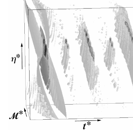
FIG. 1.: Shown here are surfaces of constant ambiguity function ${\cal A}(t^{*},{\cal M}^{*},\eta^{*})$ for the binary system $1.4M_{\odot}+10M_{\odot}$. The reference signal is a one-mode signal, and the templates are second post-Newtonian waveforms. The light grey surfaces represent ${\cal A}=15\%$, the dark grey surfaces represent ${\cal A}=30\%$, and the black surfaces represent ${\cal A}=50\%$. The global maximum of 95.5% is contained within the large structure to the left of the box. The other structures contain additional local maxima, and these make an automated search for the true maximum difficult. The region of parameter space covered by the box is $-0.06<t^{*}<0.35$, $0.96<{\cal M}^{*}<1.05$, and $0.35<\eta^{*}<0.90$.

We now discuss the issue of maximizing the ambiguity function over the template parameters. Maximization over $\phi^{*}$ is straightforward. Since $\phi^{*}$ comes as an overall phase in $\tilde{h}(f;\mathchoice{{\hbox{\boldmath$\displaystyle\theta$}}}{{\hbox{\boldmath$\textstyle\theta$}}}{{\hbox{\boldmath$\scriptstyle\theta$}}}{{\hbox{\boldmath$\scriptscriptstyle\theta$}}})$, we have that $(s|h)=\mbox{Re}(|I|e^{i\alpha})$, where $\alpha$ is linear in $\phi^{*}$, and where $I$ is some function of the remaining parameters. Maximization over $\phi^{*}$ is achieved by making $\alpha=0$, which yields $(s|h)=|I|$. Since $(h|h)$ and $(s|s)$ do not depend on $\phi^{*}$, we have also maximized ${\cal A}(\mathchoice{{\hbox{\boldmath$\displaystyle\theta$}}}{{\hbox{\boldmath$\textstyle\theta$}}}{{\hbox{\boldmath$\scriptstyle\theta$}}}{{\hbox{\boldmath$\scriptscriptstyle\theta$}}})$ over $\phi^{*}$. We will denote this reduced ambiguity function by ${\cal A}(t^{*},{\cal M}^{*},\eta^{*})$. Maximizing this over the remaining parameters is not a straightforward numerical problem, because the ambiguity function displays a very rich structure, featuring many local minima and maxima (see Fig. 1). We proceed as follows. For each binary system under consideration we evaluate the reduced ambiguity function in a fairly large neighborhood of $(t^{*},{\cal M}^{*},\eta^{*})=(0,1,1)$. The function is then displayed graphically with the help of a three-dimensional visualization software [32], and the approximate position of the global maximum is determined. Finally, the maximum is determined accurately by applying Powell’s method as described in the book Numerical Recipes [33]. The value of ${\cal A}(t^{*},{\cal M}^{*},\eta^{*})$ at the global maximum is the fitting factor FF.

The calculations described in this section require a great deal of numerical work. To minimize the possibility of making coding errors which would affect our results and conclusions, a separate code was written by each of the authors. Because the outputs of the two separate codes agree within the numerical uncertainty quoted in the caption of Table II, we are quite confident in the accuracy of our results.

V Results and discussion

Our results are displayed in Table II. For each binary system we consider two types of signals. The one-mode signal contains only the $l=m=2$ mode, while the $l\leq 3$ signal contains all modes up to $l=3$. Inclusion of additional modes does not change the results within the numerical uncertainty. We see that the fitting factors for the one-mode signals are large, all above approximately 95%. However, inclusion of additional modes decrease the fitting factors appreciably: the reduction ranges from approximately 3% for low-mass systems to approximately 7% for large-mass systems. We have verified that most of this reduction can be attributed to the $l=m=3$ mode. Nevertheless, the fitting factors are all larger than 90%, except for the large-mass system $4M_{\odot}+30M_{\odot}$. The second post-Newtonian templates therefore meet the Apostolatos criterion [14], and we conclude that they should be adequate to search for gravitational waves emitted during the adiabatic inspiral of a compact binary system.

TABLE III.: Searching a one-mode signal with Newtonian templates. For each binary system we list the values of ${\cal M}^{*}$ and $t^{*}$ corresponding to the global maximum of ${\cal A}(t^{*},{\cal M}^{*})$. The fitting factor is also listed. The numerical uncertainties are as in Table II.

System	${\cal M}^{*}_{\rm max}$	$t^{*}_{\rm max}$	FF
$1.4+1.4$	0.9944	$-0.4120\times 10^{-3}$	79.2%
$0.5+5$	0.9999	$-0.3597\times 10^{-4}$	51.6%
$1.4+10$	1.0201	$-0.1057\times 10^{-2}$	55.8%
$10+10$	1.0563	$-0.1361\times 10^{-1}$	70.1%
$4+30$	1.1503	$-0.2339\times 10^{-1}$	61.3%

For comparison, we show in Table III the results obtained when Newtonian templates are used. [We discard all post-Newtonian corrections in Eq. (12), and $\eta^{*}$ disappears from the list of template parameters.] Here the fitting factors are computed using a one-mode signal, as this gives the largest result. We see that these fitting factors are all much smaller than those of Table II. The Newtonian templates do not meet the Apostolatos criterion [14].

The reduction in fitting factor that occurs when a one-mode signal is replaced by a $l\leq 3$ signal is clearly caused by the template’s inability to keep track of the additional frequency components. We have attempted to improve the performance of our templates by adding a term

$$\tilde{h}_{3}(f;\mathchoice{{\hbox{\boldmath$\displaystyle\theta$}}}{{\hbox{\boldmath$\textstyle\theta$}}}{{\hbox{\boldmath$\scriptstyle\theta$}}}{{\hbox{\boldmath$\scriptscriptstyle\theta$}}})\propto\frac{3^{7/3}}{2^{10/3}}\,(1-4\eta)^{1/2}\,f^{-7/6}\,x\,\sin\theta\,e^{i[2\pi ft_{c}-3\phi_{c}/2+\phi(2f/3)]},$$ (17)

where the constant of proportionality is the same as in Eq. (10). While $\tilde{h}(f;\mathchoice{{\hbox{\boldmath$\displaystyle\theta$}}}{{\hbox{\boldmath$\textstyle\theta$}}}{{\hbox{\boldmath$\scriptstyle\theta$}}}{{\hbox{\boldmath$\scriptscriptstyle\theta$}}})$ describes waves at twice the orbital frequency and is the leading-order term in a post-Newtonian expansion, $\tilde{h}_{3}(f;\mathchoice{{\hbox{\boldmath$\displaystyle\theta$}}}{{\hbox{\boldmath$\textstyle\theta$}}}{{\hbox{\boldmath$\scriptstyle\theta$}}}{{\hbox{\boldmath$\scriptscriptstyle\theta$}}})$ describes waves at three times the orbital frequency and is a correction term of order $v$. Equation (17) was obtained by Fourier transforming Eq. (3b) of Ref. [9]. Our expectation was that this additional term would do a good job at reproducing the behavior of the $l=m=3$ mode, and that the loss in FF would be regained. Calculating fitting factors with $h+h_{3}$ as templates shows otherwise. (Some thought must be given to the fact that $\phi^{*}$ no longer appears as an overall phase in the templates.) The improvement in FF was less than 1% for the large-mass systems, and less than 0.1% for the low-mass systems. This prompts us to conclude that it would be pointless to introduce additional frequency components in the search templates.

It is interesting to observe that for low-mass systems, the maximum of the ambiguity function is obtained when ${\cal M}$ is approximately 0.1% above its actual value, while $\eta$ is approximately 40% of its actual value. These numbers can be loosely interpreted as the systematic errors incurred when attempting to estimate the source parameters with imperfect 2PN templates. The systematic errors should be compared with the anticipated statistical uncertainties associated with the measurement of a noisy signal [15, 21, 31, 34]. Cutler and Flanagan [15] have determined that for low-mass systems known to be composed of nonrotating companions, the statistical uncertainty associated with the estimation of ${\cal M}$ is of the order of 0.005%, while it is of the order of 1% for $\eta$ [35]. (This assumes detection with a signal-to-noise ratio of 10.) Second post-Newtonian templates therefore give rise to systematic errors that are much larger than the statistical uncertainties. While these templates could be adequate to search for signals, they should not be used as measurement templates.

REFERENCES

- [1] A. Abramovici, W.E. Althouse, R.W.P. Drever, Y. Gürsel, S. Kawamura, F.J. Raab, D. Shoemaker, L. Sievers, R.E. Spero, K.S. Thorne, R.E. Vogt, R. Weiss, S.E. Whitcomb, and M.E. Zucker, Science 256, 325 (1992).
- [2] C. Bradaschia, R. Del Fabbro, A. Di Virgilio, A. Giazotto, H. Kautzky, V. Montelatici, D. Passuello, A. Brillet, O. Cregut, P. Hello, C.N. Man, P.T. Manh, A. Marraud, D. Shoemaker, J.Y. Linet, F. Barone, L. Di Fiore, L. Milano, G. Russo, J.M. Aguirregabiria, H. Bel, J.P. Duruisseau, G. Le Denmat, Ph. Tourrenc, M. Capozzi, M. Longo, M. Lops, I. Pinto, G. Rotoli, T. Damour, S. Bonazzola, J.A. Marck, Y. Gourghoulon, L.E. Holloway, F. Fuligni, V. Iafolla, and G. Natale, Nucl. Instrum. & Methods A289, 518 (1990).
- [3] For an overview, see B.F. Schutz, in The Detection of Gravitational waves, edited by D.G. Blair (Cambridge University Press, Cambridge, England, 1991), p. 406.
- [4] C. Cutler, T.A. Apostolatos, L. Bildsten, L.S. Finn, E.E. Flanagan, D. Kennefick, D.M. Markovic, A. Ori, E. Poisson, G.J. Sussman, and K.S. Thorne, Phys. Rev. Lett. 70, 2984 (1993).
- [5] E.S. Phinney, Astrophys. J. 380, L17 (1991).
- [6] R. Narayan, T. Piran, and A. Shemi, Astrophys. J 379, L17 (1991).
- [7] A.V. Tutukov and L.R. Yungelson, Mon. Not. Roy. Astron. Soc. 260, 675 (1993).
- [8] L.A. Wainstein and V.D. Zubakov, Extraction of Signals from Noise (Prentice-Hall, Englewood Cliffs, 1962).
- [9] L. Blanchet, B.R. Iyer, C.M. Will, and A.G. Wiseman, Class. Quantum Grav. 13, 575 (1996).
- [10] L. Blanchet, Phys. Rev. D 54 1417 (1996).
- [11] E. Poisson, Phys. Rev. D 52, 5719–5723 (1995). Erratum and Addendum, Phys. Rev. D 55, June 15 (1997).
- [12] L.E. Simone, S.W. Leonard, E. Poisson, and C.M. Will, Class. Quantum Grav. 14, 237 (1997).
- [13] Here and below, the signal-to-noise ratio is defined to be the expectation value of the maximum correlation between the noisy detector output and the templates.
- [14] T.A. Apostolatos, Phys. Rev. D 52, 605 (1996).
- [15] C. Cutler and E.E. Flanagan, Phys. Rev. D 49, 2658 (1994).
- [16] B.S. Sathyaprakash and S.V. Dhurandhar, Phys. Rev. D 44, 3819 (1991).
- [17] S.V. Dhurandhar and B.S. Sathyaprakash, Phys. Rev. D 49, 1707 (1994).
- [18] R. Balasubramanian and S.V. Dhurandhar, Phys. Rev. D 50, 6080 (1994).
- [19] B.S. Sathyaprakash, Phys. Rev. D 50, 7111 (1994).
- [20] R. Balasubramanian, B.S. Sathyaprakash, and S.V. Dhurandhar, Phys. Rev. D 53, 3033 (1996).
- [21] A. Królak, Estimation of the post-Newtonian parameters in the gravitational-wave emission of a coalescing binary to 5/2pN order (unpublished).
- [22] S.A. Teukolsky, Astrophys. J. 185, 635 (1973).
- [23] E. Poisson, Phys. Rev. D 47, 1497 (1993).
- [24] C. Cutler, L.S. Finn, E. Poisson, and G.J. Sussman, Phys. Rev. D 47, 1511 (1993).
- [25] B.J. Owen, Phys. Rev. D 53, 6749 (1996).
- [26] T.A. Apostolatos, Phys. Rev. D 54, 2421 (1996).
- [27] T.A. Apostolatos, C. Cutler, G.J. Sussman, and K.S. Thorne, Phys. Rev. D 49, 6274 (1994).
- [28] J.N. Goldberg, A.J. MacFarlane, E.T. Newman, F. Rohrlich and E.C.G. Sudarshan, J. Math. Phys. 8, 2155 (1967).
- [29] K.S. Thorne, in 300 Years of Gravitation, edited by S.W. Hawking and W. Israel (Cambridge University Press, Cambridge, England, 1987), p. 330.
- [30] A. Apostolatos, D. Kennefick, A. Ori, and E. Poisson, Phys. Rev. D. 47, 5376 (1993).
- [31] E. Poisson and C.M. Will, Phys. Rev. D 52, 848 (1995).
- [32] The software is vis5d, and is available free of charge from http://www.scsc.edu/~michaels/vizwiz.html.
- [33] W.H. Press, B.P. Flannery, S.A. Teukolsky, and W.T. Vetterling, Numerical Recipes (Cambridge University Press, Cambridge, England, 1986).
- [34] R. Balasubramanian and S.V. Dhurandhar, Gravitational waves from coalescing binaries: Estimation of parameters (unpublished; gr-qc/9702015).
- [35] Cutler and Flanagan derived these results using a 1.5PN waveform. We have recalculated the statistical uncertainties using a 2PN waveform, and have found the same answer.