Spherical Collapse of a Mass-Less Scalar Field With Semi-Classical Corrections

Abstract

We investigate numerically spherically symmetric collapse of a scalar field in the semi-classical approximation. We first verify that our code reproduces the critical phenomena (the Choptuik effect) in the classical limit and black hole evaporation in the semi classical limit. We then investigate the effect of evaporation on the critical behavior. The introduction of the Planck length by the quantum theory suggests that the classical critical phenomena, which is based on a self similar structure, will disappear. Our results show that when quantum effects are not strong enough, critical behavior is observed. In the intermediate regime, evaporation is equivalent to a decrease of the initial amplitude. It doesn’t change the echoing structure of near critical solutions. In the regime where black hole masses are low and the quantum effects are large, the semi classical approximation breaks down and has no physical meaning.

1 Introduction

Spherical symmetric collapse of a scalar field was studied analytically by Christodoulou [1] who concluded that for near trivial initial data, the field disperses to future null infinity leaving an empty space-time, and for “stronger” initial data, the field implosion forms a black-hole. This result was verified numerically by Goldwirth & Piran [2]. If we now characterize the “strength” of the initial data by some well defined parameter $p$ which is monotonously growing with the “strength” (e.g. the initial amplitude of the field), we can expect that there will exist a critical value $p^{*}$ so that data with $p<p^{*}$ disperses while data with $p>p^{*}$ creates a black-hole. An intriguing question is what happens at $p=p^{*}$. This question was investigated numerically by Choptuik [3]. His findings were

• In the limit $p\rightarrow p^{*}$ the asymptotic behavior of the scalar field and the metric is universal - independent of the initial profile of the field. The field and metric also posses a symmetry - discrete self similarity (DSS) in the neighborhood of the critical solution’s horizon.

• The DSS is a periodical behavior at the origin with exponentially smaller periods in proper time: $\tau\mapsto\tau e^{-\Delta}$ where $\tau=t^{*}-t$, $t^{*}$ being the time of formation of the critical black-hole, $\Delta\approx 3.44$.

• The mass of the black hole formed by marginally supercritical data has a scaling law $M\propto(p-p^{*})^{\gamma}$ with $\gamma\approx 0.375$.

Perhaps one of the striking conclusions from these findings is that it is possible to produce a black-hole with an infinitesimal mass. The limiting case zero mass black-hole, the “choptuon” can be viewed as a collapsing ball of field energy for which the rate of collapse is exactly balanced by the energy loss by radiation, so that when the ball shrinks to zero radius all of its energy is radiated away [4]. The choptuon is actually a naked singularity, visible from null infinity [5] although it is not generic and it is destroyed by an arbitrarily small perturbation.

Hawking [6] has shown that within the semi-classical approximation black holes evaporate thermally. The rate of evaporation depends on the black hole’s mass via the relation [7]:

$$\frac{\partial M}{\partial t}\propto-M^{-2},$$ (1)

with the proportionality constant depending on the number of particle species that can be emitted by the black-hole at a given temperature. Integration of this relation yields a black-hole lifetime which is proportional to $M^{3}$. This suggests that quantum effects will change the Choptuik effect since infinitesimally small black holes evaporate almost instantly.

The semi-classical approach to gravitation stipulates that we can write the semi-classical Einstein equation [8]

$$G_{\mu\nu}=8\pi{\langle T^{Q}\rangle}_{\mu\nu},$$ (2)

where $\langle T^{Q}\rangle$ is the expectation value of the effective quantum energy-momentum tensor. This approach has been tested to give rise to evaporation of the black hole satisfying Eq. (1) in [9].

We explore the evaporation of a black hole formed by collapse of a scalar field and the effect of the evaporation on the Choptuik phenomena. To this end, we investigate, numerically, the spherical collapse of a scalar field with the addition of an appropriate $\langle T^{Q}\rangle$. We use $\langle T^{Q}\rangle$ adapted from a 2D expectation value that reproduces the Hawking radiation [9]. This in turn forces us to solve the evolution equations. This is significantly harder in our coordinates then the usual method of solving the constraint equations used in [10] and [5]. In fact, this is the first time that a numerical solution using the evolution equations has been presented. Another problem with the above $\langle T^{Q}\rangle$ is that the tensor is divergent at the origin. We renormalize the tensor to bypass this problem. This renormalization violates the Bianchi identity near the origin however the semi classical approximation is not valid there anyway. The code is tested with the classical problem to reproduce the Choptuik effect. After this we check black hole evaporation. Finally we examine the effect of evaporation on the Choptuik phenomena.

The introduction of quantum effects via $\langle T^{Q}\rangle$ immediately introduces the Planck length scale denoted here by $\sqrt{\alpha}$. The addition of a length scale to the previously scale-less problem of the massless scalar field suggests that the critical phenomena present there will disappear [11]. However, our results show that the critical phenomena does not disappear within the regime of validity of the semi-classical approximation.

We discuss the problem of classical & semi-classical scalar field collapse in Sec. II & III. Our numerical scheme is described in Sec. IV and our results in Sec. V. In Sec. VI we summarize our findings. Finally in Appendix A we derive several auxiliary quantities needed for the numerical scheme.

2 Classical Scalar Field Collapse

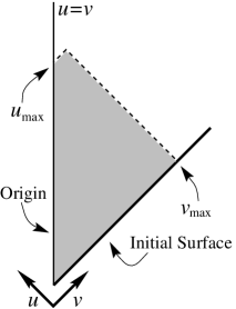
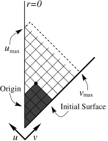
a b

Figure 1: (a) The boundaries of the computational region. Initial values are given on the initial surface and boundary conditions on the origin. The shaded area is the integration area. (b) The grid defined by double null coordinates. The casual past of some point $p$ is shaded

The characteristics of a massless scalar field are null so a double null coordinate system $u,v$ is the ”natural” system for this problem. In these coordinates the horizon (when it forms) is regular and there are no coordinate singularities. This enables us to study quantum effects that occur near the horizon.

The metric is:

$$ds^{2}=e^{2f}dudv-r^{2}d\Omega^{2},$$ (3)

Where $f$ and $r$ are functions of $u$ and $v$ only. This definition is only unique up to a change of variables $v^{\prime}=f_{1}(v),u^{\prime}=f_{2}(u)$. This ambiguity can be settled by a choice of the origin ($r=0$) as $u=v$ and by choosing either $r$ or $f$ on the initial surface. We choose $r=\frac{1}{2}v$ on $u=0$ which is supposed to be sufficiently far in the past. This choice corresponds to an asymptotically flat space-time. Regularity of the origin, with the above choice of coordinates, implies the following boundary conditions:

$$r_{,v}\Big{|}_{r=0} = -r_{,u}\Big{|}_{r=0},$$ (4a)

$$\phi_{,v}\Big{|}_{r=0} = \phi_{,u}\Big{|}_{r=0},$$ (4b)

$$f_{,v}\Big{|}_{r=0} = f_{,u}\Big{|}_{r=0}.$$ (4c)

The Classical Einstein equations together with the field’s equation of motion can be divided into two types: The dynamical equations

$$r_{,uv} = -\frac{\eta r}{2},$$ (5a)

$$f_{,uv} = -4\pi\phi_{,u}\phi_{,v}+\frac{\eta}{2},$$ (5b)

$$\phi_{,uv} = -\frac{1}{r}\left({r_{,u}\phi_{,v}+r_{,v}\phi_{,u}}\right)$$ (5c)

and the constraint equations:

$$-r_{,vv}+2f_{,v}r_{,v} = 4\pi r\phi_{,v}^{2},$$ (6a)

$$-r_{,uu}+2f_{,u}r_{,u} = 4\pi r\phi_{,u}^{2}.$$ (6b)

We have introduced here the auxiliary quantity $\eta$,

$$\eta\equiv\frac{1}{r^{2}}\left(2r_{,u}r_{,v}+\frac{1}{2}e^{2f}\right)=e^{2f}\frac{m}{r^{3}},$$ (7)

where $m(u,v)$, is the mass inside a sphere of radius $r(u,v)$:

$$m=\frac{r}{2}\left(1+4r_{,u}r_{,v}e^{-2f}\right).$$ (8)

3 Black Hole Evaporation & The Semi-Classical Approximation

We add to the classical equations an effective stress energy tensor $\langle T^{Q}\rangle$ that describes the evaporation. Following [9] we turn to 2D theories to obtain a tensor embodying Hawking radiation and adapt it to 4D. The expectation value of the 2D quantum energy-momentum tensor [12], in double-null coordinates, is divided by $4\pi r^{2}$ to mimic the 4D radial dependence to give:

$${\langle T^{Q}\rangle}_{\mu\nu}=\frac{\alpha}{4\pi r^{2}}\left[\begin{array}[]{cccc}f_{,uu}-f_{,u}^{2}&-f_{,uv}&0&0\\ -f_{,uv}&f_{,vv}-f_{,v}^{2}&0&0\\ 0&0&0&0\\ 0&0&0&0\end{array}\right]$$ (9)

The constant $\alpha$ defines a length scale $\sqrt{\alpha}$ which is of the order of the Planck scale. Beyond this scale the semi-classical approximation it is not valid.

Unfortunately this tensor diverges at the origin. Note that for a null fluid considered by [9], the origin is always flat and $\langle T^{Q}\rangle$ vanishes identically there. Any attempt to regularise this tensor must take into account that this tensor must be divergence-less (i.e. $\nabla{\langle T^{Q}\rangle}=0$) because of the Bianchi identity. A simple attempt to renormalize $\langle T^{Q}\rangle$ by multiplying it by a general function $Q(r)$ fails, we find that the Bianchi identity is violated unless $Q={\rm Const}$. Other attempts which were based on an introduction of angular terms failed as well and we had no choice but to ignore the Bianchi identity following [9] and to multiply $\langle T^{Q}\rangle$ by

$$Q=\frac{\alpha/r^{2}}{1+\left(\alpha/r^{2}\right)^{2}}.\\$$ (10)

The deviation from the Bianchi identity is significant only for $r\hbox{\hbox to0.0pt{${}^{<}$\hss}${}_{\sim}$}\sqrt{\alpha}$, for which the whole the semi classical approximation is no longer valid anyway.

The resulting semi-classical dynamical equations are:

$$r_{,uv} = \frac{r}{(1-Q)}\left({4\pi Q\phi_{,u}\phi_{,v}-\frac{\eta}{2}}\right),$$ (11a)

$$f_{,uv} = \frac{1}{(1-Q)}\left({-4\pi\phi_{,u}\phi_{,v}+\frac{\eta}{2}}\right),$$ (11b)

$$\phi_{,uv} = -\frac{1}{r}\left({r_{,u}\phi_{,v}+r_{,v}\phi_{,u}}\right),$$ (11c)

and the constraint equations are:

$$-r_{,vv}+2f_{,v}r_{,v} = 4\pi r\phi_{,v}^{2}+Qr\left({f_{,vv}-f_{,v}^{2}}\right),$$ (12a)

$$-r_{,uu}+2f_{,u}r_{,u} = 4\pi r\phi_{,u}^{2}+Qr\left({f_{,uu}-f_{,u}^{2}}\right).$$ (12b)

4 Numerical Scheme

a b

Figure 2: (a) The regular grid structure away from the origin. The source terms are calculated at $\rm s_{1}$ and $\rm s_{2}$. $\eta$ is integrated along the dashed line and the derivatives are calculated at $\rm p_{1}$, $\rm p_{2}$ in the first iteration. (b) A typical grid arrangement near the origin. The point $p$ is interpolated. Notice that $du\neq dv$ (e.g. cell 1-2-2’-1’) and that the first rectangular cell might differ from the rest of the cells (e.g 0-1-1’-p as compared to 1-2-2’-1’). Points -1 and -1’ are “fake” points calculated from the symmetry conditions.

We choose $u=0$ as our initial surface and use the constraint equation Eq. (12a) to determine the value of $f$ given $r$ and $\phi$ on this line. The integration proceeds, for each constant $u$, line from the origin $v=u$, where the boundary conditions Eq. (3) are imposed, up to $v_{\rm max}$ which is an arbitrarily chosen maximal value of $v$. In this way, the complete casual past of each point is known when the integration routine has to determine the field’s value at that point.

The straightforward numerical scheme becomes unstable once the gravitational effects become important ($\frac{2m}{r}\sim 1$). To stabilize the scheme, we have introduced the auxiliary quantity $\eta$ Eq. (7) which is integrated on constant $u$ lines. We use this value of $\eta$ in the source for the evolution equations. It is worth noting that $\eta$ needs to be accurate only to first order since it is a source term. This modification stabilizes the scheme. This is the first numerical scheme to solve this problem using the evolution equations in double null coordinates.

A grid refinement algorithm was used in order to increase resolution at specific places such as the near-critical solutions and at the evaporation stage of the black-hole.

We take $u=0$ to be the initial surface. On this surface, we specify an initial value for the scalar field $\phi$. Then we choose $r=\frac{1}{2}v$ on the initial surface and solve Eq. (12a) for $f$. The quantum terms should be negligible on the initial surface, so they were ignored while solving for $f$. We later verify that these terms are indeed negligible. The initial value equation for $f$ is

$$f_{,v}=2\pi\frac{r}{r_{,v}}\phi_{,v}^{2}=2\pi v\phi_{,v}^{2},$$ (13)

with $f(0,0)=0$ as a boundary condition. Eq. (13) is integrated using a fourth order Runge-Kutta algorithm.

Once the values of the fields on $u=0$ are known the integration proceeds as follows: (all references to grid points and cells are illustrated in Fig. (2))

The first step involves a triangular cell on the origin. Here we utilize the boundary conditions Eq. (3). Because space-time is flat near the origin, the $r$ direction is $(1,-1)$ when taken as a vector in the $(v,u)$ plane. Thus we can approximate $\frac{\partial\phi}{\partial r}$ to order $(\Delta r)^{2}$ in the current step by using the value of $\phi$ at the two last steps.

• Using the value of $\phi_{1^{\prime}}$ and $\phi_{3^{\prime\prime}}$ we obtain the value of $\phi_{0}$.

• Once the value of $\phi_{0}$ is known, $\phi_{,v}$ and $\phi_{,uv}$ are calculated on the origin between the points 0 and 0’ using also $\phi_{-1}=\phi_{p}$ (again using Eq. (3) and $\phi_{0^{\prime}}$).

• Now we calculate the value of $f_{,uv}=\eta/2=4\pi/3\phi_{,v}^{2}$ and using the known $f_{0^{\prime}}$ and $f_{-1}=f_{p}$ we obtain $f_{0}$

• Finally we calculate $f_{,v}$ at the same point as $\phi_{,v}$ and $\phi_{,uv}$ and from them $\eta$ and $\eta_{,v}$ using Eq. (28) and Eq. (31) (see appendix A for derivation of these equations).

All interpolations are done using a third degree polynomial such that the point being interpolated always has two known points on each side (e.g. the values $z_{-1^{\prime}},z_{0^{\prime}},z_{1^{\prime}}$ and $z_{2^{\prime}}$ are used to interpolate $z_{p}$).

Away from the origin we have rectangular cells. For each step in the $v$ direction three points are known (from previous steps) and the fourth (the future-most) is calculated (e.g $z_{2},z_{2^{\prime}}$ and $z_{3^{\prime}}$ are known and $z_{3}$ is calculated). The integration is a two step iterative procedure. The basic principle is that the second derivative operator can be discretesized as follows:

$$z_{,uv}\Big{|}_{s_{2}}=\frac{z_{3}-z_{2}-z_{3^{\prime}}+z_{2^{\prime}}}{\Delta u\Delta v}+O((\Delta u\Delta v)^{2})$$ (14)

The source terms of the equations are split into two - the gravitational term involving $\eta$ and the field term. The gravitational term is integrated along a constant $u$ line which runs through the point at which the source is calculated (in between of the grid-lines). The field term is calculated directly.

$\bf 1^{\bf st}$ Iteration

The fields and their derivatives at point $s_{2}$ are approximated using the known values at 2,2’ and 3’:

$$z\Big{|}_{s_{2}} \approx \frac{1}{3}(z_{2}+z_{2^{\prime}}+z_{3^{\prime}})$$ (15)

$$z_{,v}\Big{|}_{s_{2}} \approx \frac{1}{\Delta v}(z_{3^{\prime}}-z_{2^{\prime}})$$ (16)

$$z_{,u}\Big{|}_{s_{2}} \approx \frac{1}{\Delta u}(z_{2}-z_{2^{\prime}})$$ (17)

$\eta$ is integrated using $\eta_{,v}\Big{|}_{s_{1}}$ calculated for the previous point. Eq. (14) yields a first approximation for $z_{3}$.

$\bf 2^{\bf nd}$ Iteration

A second order approximation for the fields and their derivatives can now be obtained using $z_{3}$ calculated in the first iteration:

$$z\Big{|}_{s_{2}} \approx \frac{1}{4}(z_{2}+z_{3}+z_{2^{\prime}}+z_{3^{\prime}}),$$ (18)

$$z_{,v}\Big{|}_{s_{2}} \approx \frac{1}{2\Delta v}(z_{3^{\prime}}-z_{2^{\prime}}+z_{3}-z_{2}),$$ (19)

$$z_{,u}\Big{|}_{s_{2}} \approx \frac{1}{2\Delta u}(z_{2}-z_{2^{\prime}}+z_{3}-z_{3^{\prime}}).$$ (20)

An improved approximation for $\eta$ is given by:

$$\eta_{,v}\Big{|}_{p_{1}}\approx\frac{1}{2}\left(\eta_{,v}\Big{|}_{s_{1}}+\eta_{,v}\Big{|}_{s_{2}}\right).$$ (21)

This iterative explicit scheme gives us a second order accuracy.

To study the last stages of collapse, we utilize a cell refinement algorithm that increases the resolution of the integration in the areas of interest. Various multi grid or adaptive mesh [13] methods have been used to study critical collapse (cf. [3] and [5]) but the increased complexity of these schemes was unnecessary for our purpose. We chose to half the value of $\Delta u$ at preset intervals, keeping the value of $\Delta v$ constant. This scheme has the advantage that we can reach an asymptotic value of $u$ which is independent of the value of $v_{\rm max}$. Using it we can study structure away from the origin. The price is that the first rectangular cell can be different from the others (see Fig. 2b). This scheme also sacrifices $v$ resolution. Both problems are not critical.

5 Results

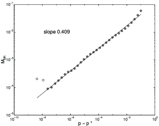
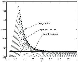
a b

Figure 3: Classical results: (a) A log-log plot of $M_{\rm bh}$ vs. $p-p^{*}$. The slope, 0.409, is higher then the usually quoted result of 0.375. Both the slope and $p^{*}$ were found through least squares fitting. (b) A contour plot of $r$ values in the case of formation of a black hole. The event horizon, apparent horizon & the singularity are marked. The apparent horizon is always beyond (larger $u$) the event horizon.

To test our code we first ran it on the classical ($\sqrt{\alpha}=0$) problem. We find a critical initial amplitude $p^{*}$. For initial data with amplitudes smaller then $p^{*}$ the field disperses leaving a flat space-time. For initial amplitudes above $p^{*}$ the field collapses to form a black hole. For amplitudes near $p^{*}$ the solution exhibits self similar oscillations. A log-log plot of $M_{\rm bh}$ as a function of $p-p^{*}$ can be seen in Fig. (3). Although the critical exponent we found, $\gamma=0.409$ is larger then the usually quoted number $\gamma\approx 0.375$ the power law dependence of $M_{\rm bh}$ on $p-p^{*}$ is evident. Thus our code reproduces the classical behavior. The discrepancy in the value of $\gamma$ reflects the accuracy of the code. We also present a contour plot of $r$ showing the apparent horizon, the singularity and the event horizon (defined as the last ray to avoid the singularity). For the classical case, the apparent horizon is always inside the event horizon - any photon which starts falling into the black hole will never escape.

The introduction of $\langle T^{Q}\rangle$ creates an effective outgoing flux corresponding to Hawking radiation. This flux produces an evaporation satisfying Eq. (1) as verified in [9] for black holes created by a null fluid. It is sometimes hard to distinguish the evaporation from the energy momentum of the scalar field which is reflected from the origin. These reflections and the tail of the incoming scalar field can mask the quantum flux. To see a distinct black hole evaporation we need to create a situation where the only energy flux crossing the horizon is the outgoing Hawking radiation. This can be accomplished by looking at initial conditions that create a black hole before a significant fraction of the scalar field’s energy is reflected from the origin. We also look for conditions producing an apparent horizon after most of the field has collapsed (large $v$) so that the tail of the field is also inside the horizon.

a

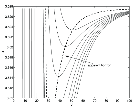
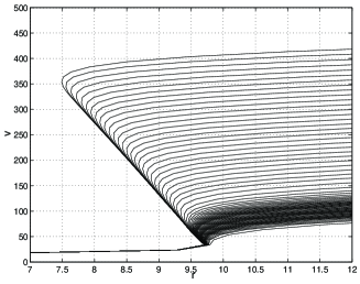
b c

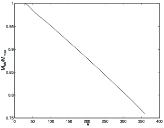
Figure 4: (a) Contour of $r$ in the evaporation region. The field is centered around $v=20$, to the left of it the space time is flat ($r\propto v-u$). The dotted line describes $r_{,v}=0$ - the apparent horizon. The event horizon is at the top of the graph ($u=3.528$). (b) trajectories of $r(v)$ for different values of $u$. These null trajectories curve back towards the singularity but then turn around and escape to infinity. This is a clear indication for mass decrease. The decrease in radius of the apparent horizon is evident. (c) The black hole’s mass as function of $v$. A 25% decrease in mass is evident.

Fig. (4) depicts the geometry resulting from the evolution of a scalar field with such initial conditions. In the $r$ contour plot Fig. (4a) The appearance of the apparent horizon before (lower $u$) the event horizon is apparent. Null trajectories which begin to curve back towards the singularity but then turn around and escape to infinity are shown in the $r(v)$ plot Fig. (4b). The evaporation of the black hole is indicated by the decreasing radius of the outer apparent horizon which implies a negative energy flux through the apparent horizon.

It is difficult to resolve the evaporation in the $u,v$ coordinates which constitute the inertial frame of an observer at rest on the origin. In these coordinates, the evaporation is contained within a tiny $u$ lapse. We therefore utilize the redshift of outgoing rays (as in [9]) which implies that $r_{,u}\Big{|}_{r\gg m}$ diverges as the event horizon is approached. We half the $u$ step $\Delta u$ in order to always have:

$$r_{,u}\Delta u\Big{|}_{v=v_{\rm max}}<\Delta r,$$ (22)

where $\Delta r$ is the value of the lhs. of Eq. (22) for the first $u$ step. Using this scheme we managed to resolve a 25% decrease in the black hole mass due to evaporation.

In our search for the scaling law which characterizes the Choptuik phenomena, we have to stop when the resulting black hole mass approaches $\sqrt{\alpha}$. Nevertheless, we can still take $\alpha\ll 1$ and try to get a scaling law down to the minimal meaningful mass.

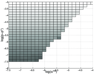
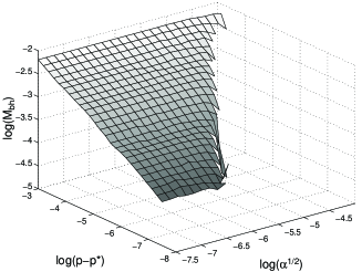
Figure 5: $M_{\rm bh}$ as function of $\sqrt{\alpha}$ and $p-p^{*}$ Darker colors indicate lower mass. As $\sqrt{\alpha}$ increases $M_{\rm bh}$ decreases until finally no black hole is formed. The empty region is where no black holes formed. The final decrease in $M_{\rm bh}$ is too rapid to be resolved in this graph

In Fig. (5) we show a plot of $M_{\rm bh}$ as a function of $p-p^{*}$ and $\sqrt{\alpha}$. For small $\sqrt{\alpha}$ the evaporation is negligible and we recover the power law dependence of $M_{\rm bh}$ on $p-p^{*}$. As we increase $\sqrt{\alpha}$ the effects of mass loss is apparent. For large values of $\sqrt{\alpha}$ black holes do not form where they would have classically. Thus, increasing $\alpha$ is effectively equivalent to decreasing $p$. This occurs because of mass loss during the evolution. These losses by evaporation can even change supercritical classical initial data into a subcritical solution and inhibit the formation of a black hole.

a
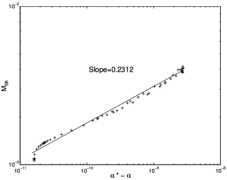
b
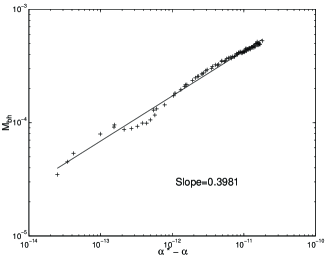
c

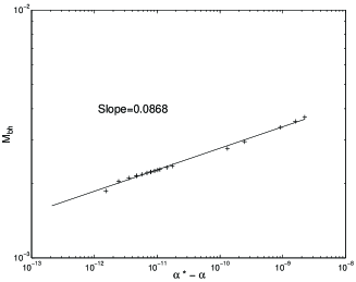
Figure 6: $M_{\rm bh}$ as function of $\alpha^{*}-\alpha$ for three different $p$. $\alpha^{*}$ was determined through fitting. The values of $\alpha^{*}$ are $3.8\times 10^{-8}$, $2.8\times 10^{-9}$ and $2.7\times 10^{-11}$ for graphs (a), (b) and (c) respectively.

The decrease in mass with increasing $\sqrt{\alpha}$ is too rapid to be resolved by the coarse grid of Fig. (5). In Figs. (6) and (7) we examine more closely the changes in the evolution due to increasing $\sqrt{\alpha}$. In Fig. (6) we show, $M_{\rm bh}$ as a function of $\sqrt{\alpha}$ for three different values of $p-p^{*}$. A power law dependence of $M_{\rm bh}$ on $\sqrt{\alpha}$ with an exponent which is dependent on the value of $p-p^{*}$ can be seen. The power law depicted in Fig. (6) is broken before the semi-classical limit is reached by a rapid fall in $M_{\rm bh}$. This feature is also present in the classical ($\alpha=0$) case indicating that we have reached our limiting resolution.

Figure 7: f and $\phi$ on origin for fixed initial data (fixed $p$) and different $\sqrt{\alpha}$. The different curves are offset vertically in order to enhance readability. Increasing $\sqrt{\alpha}$ increases the number of echoes and is thus equivalent to decreasing $p$

Fig. (7) depicts $\phi$ and $f$ on the origin for various values of $\sqrt{\alpha}$ with a fixed value of $p$. We see that the effect of increasing $\sqrt{\alpha}$ is practically similar to that of decreasing $p$. The general echoing structure of near critical solutions is conserved and the decrease in mass affects only the last echo. This is in agreement with the power law dependence of $M_{\rm bh}$ on $\sqrt{\alpha}$ since each echo is exponentially smaller then the preceding one in mass.

6 Summary

The numerical solution of spherical symmetric semi-classical scalar field collapse enabled us to study the effects of black hole evaporation on the critical phenomena present in classical collapse (the Choptuik effect). The code was tested to reproduce the critical phenomena in the classical limit and black hole evaporation in the semi classical approximation.

The addition of quantum effects and the subsequent introduction of the Planck scale $\sqrt{\alpha}$ changed the behavior of the solutions. For initial data found to form a black hole classically ($\alpha=0$) the introduction of $\sqrt{\alpha}$ caused a decrease in the resulting black hole mass $M_{\rm bh}$ . For large enough $\sqrt{\alpha}$, no black hole formed. This behavior is expected due to mass loss through evaporation. A detailed investigation of the relations between the parameters revealed that for a fixed initial data (fixed $p$) there is a power law dependence of $M_{\rm bh}$ on $\sqrt{\alpha}$. The exponent of the power law depends on $p$. Unlike some earlier expectations [11] we find that the introduction of the Planck scale does not destroy altogether the DSS behavior observed classically.

Appendix A Auxiliary Quantities

In order to carry out the numerical integration of the equations (3) we need to calculate some auxiliary quantities, mainly get an equation for $\eta_{,v}$ and get the value of $\eta$ and $\eta_{,v}$ on the origin.

Using Eq. (8) we can get an equation for $m$ from the constraint equation Eq. (12a)

$$2r_{,v}m_{,v} = 4\pi\left({1-\frac{2m}{r}}\right)r^{2}\phi_{,v}^{2}$$

$$+ \left({1-\frac{2m}{r}}\right)r^{2}Q$$

$$\times \left[{\left({f_{,vv}-f_{,v}^{2}}\right)-\frac{1}{1-Q}\left({4\pi\phi_{,u}\phi_{,v}+\frac{2m}{r^{3}}\frac{r_{,v}}{1-\frac{2m}{r}}}\right)}\right]$$

using this we can calculate $\eta$ on the origin (which is always classic)

$$m(u,v)=\int_{u}^{u+v}2\pi\left({1-\frac{2m}{r}}\right)\frac{r^{2}}{r_{,v}}\phi_{,v}^{2}dv^{\prime}$$ (24)

so by a change of variable from $v$ to $r$ at constant $u$ we have

$$m\left({u,r(u,v)}\right)=\int_{0}^{r}2\pi\left({1-\frac{2m}{r^{\prime}}}\right)\frac{{r^{\prime}}^{2}}{{r^{\prime}}_{,v}^{2}}\phi_{,v}^{2}dr^{\prime}$$ (25)

now, to the lowest order in $r$, we have (since $\frac{2m}{r}\propto o\left({r^{2}}\right)$)

$$m=2\pi\frac{\phi_{,v}^{2}}{r_{,v}^{2}}\int_{0}^{r}{r^{\prime}}^{2}dr^{\prime}$$ (26)

where all the terms out of the integral are to be evaluated at $r=0$. Using $r_{,v}^{2}=e^{2f}/4$ on the origin, we have, for small $r$

$$m\approx\frac{8\pi}{3}\phi_{,v}^{2}e^{-2f}r^{3}$$ (27)

and so, on the origin, using Eq. (7)

$$\eta=\frac{8\pi}{3}\phi_{,v}^{2}$$ (28)

to get an equation for $\eta_{,v}$, using, again, Eq. (7) we have

$$\eta_{,v}=\frac{e^{2f}}{r^{3}}\left({2mf_{,v}-3m\frac{r_{,v}}{r}+m_{,v}}\right)$$ (29)

with Eq. (7) and the quantum corrections from Eq. (A) the equation is

$$\eta_{,v} = \left({2f_{,v}-3\frac{r_{,v}}{r}}\right)\eta+\frac{2\pi}{r_{,v}}\left({\frac{e^{2f}}{r}-2\eta r}\right)\phi_{,v}^{2}$$

$$+ Q\left({\frac{e^{2f}}{r}-2\eta r}\right)$$

$$\times \left[{\left({f_{,vv}-f_{,v}^{2}}\right)-\frac{1}{1-Q}\left({4\pi\phi_{,u}\phi_{,v}+\frac{\eta r_{,v}}{e^{2f}-2\eta r^{2}}}\right)}\right]$$

We can find the value of the rhs. of Eq. (A) on the origin by expanding all the fields in powers of $v-u$. We then obtain the expansion coefficients (which depend on $u$) by substituting back into the Einstein equations Eq. (3). This is a rather tedious process but can be easily automated using symbolic math programs such as Mathematica & Maple. By comparison of coefficients we deduce that:

$$\eta_{,v}\Big{|}_{u=v}=\frac{8\pi}{3}\phi_{,v}\left({3\phi_{,uv}-2\phi_{,v}f_{,v}}\right)$$ (31)

(all quantities are evaluated at the origin).

References

- [1] Christodoulou D., Commun. Math. Phys. 109, 613 (1987)
- [2] Goldwirth D. S., Piran T., Phys. Rev. D36, 3575 (1987)
- [3] Choptuik M. W., Phys. Rev. Lett. 70, 9 (1993)
- [4] Hirschmann E., Eardly D., Phys. Rev. D52, 5850 (1995)
- [5] Hamadé R. S., Stewart J. M., Class. Quantum Gravity 31, 1 (1996)
- [6] Hawking S. W., Nature 248, 30 (1974)
- [7] Page D. N., Phys. Rev. D13, 198 (1976)
- [8] Birrell N., Davies P. W. C., Quantum Fields in Curved Spaces (Cambridge University Press, Cambridge, 1972)
- [9] Parentani R., Piran T., Phys. Rev. Lett. 73, 2805 (1994)
- [10] Garfinkle D., preprint gr-qc/9412008
- [11] Chiba T., Siino M. preprint KUNS 1384 (1996)
- [12] Davies P. C. W., Fulling S. A., Unruh W. G., Phys. Rev D13, 2720 (1976)
- [13] Berger M. J., Oliger J., J. Comput. Phys. 53, 484 (1984)