Gravitational vacuum polarization IV:
Energy conditions in the Unruh vacuum

Abstract

Building on a series of earlier papers [gr-qc/9604007,9604008,9604009], I investigate the various point-wise and averaged energy conditions in the Unruh vacuum. I consider the quantum stress-energy tensor corresponding to a conformally coupled massless scalar field, work in the test-field limit, restrict attention to the Schwarzschild geometry, and invoke a mixture of analytical and numerical techniques. I construct a semi-analytic model for the stress-energy tensor that globally reproduces all known numerical results to within $0.8\%$, and satisfies all known analytic features of the stress-energy tensor. I show that in the Unruh vacuum (1) all standard point-wise energy conditions are violated throughout the exterior region—all the way from spatial infinity down to the event horizon, and (2) the averaged null energy condition is violated on all outgoing radial null geodesics. In a pair of appendices I indicate general strategy for constructing semi-analytic models for the stress-energy tensor in the Hartle–Hawking and Boulware states, and show that the Page approximation is in a certain sense the minimal ansatz compatible with general properties of the stress-energy in the Hartle–Hawking state.

PACS: 04.60.+v 04.70.Dy

1 Introduction

It is well-known that a quantum field theory constructed on a curved background spacetime experiences gravitationally induced vacuum polarization. This effect typically induces a non-zero vacuum expectation value for the stress-energy tensor [1, 2, 3, 4, 5, 6]. It is also well-known that this gravitationally induced vacuum polarization will induce violations of at least some of the energy conditions of classical general relativity [6, 7, 8, 9, 10].

In earlier publications, I addressed these issue in some depth for both the (3+1) Hartle–Hawking vacuum [8] and (3+1) Boulware vacuum [9], and also presented an analysis for a (1+1)-dimensional toy model for which the exact analytic form of the stress-energy tensor is known [10]. For the (3+1) Unruh vacuum there are additional subtleties that must be addressed. The complications arise from two sources:

1. For the (3+1) Unruh vacuum we do not have any approximate analytic expression for the stress-energy tensor. Nothing along the lines of the Page approximation for the (3+1) Hartle–Hawking vacuum [11], or the Page–Brown–Ottewill approximation for the (3+1) Boulware vacuum [12], has yet been developed for the (3+1) Unruh vacuum.

2. If we resort to numerical methods, using the numerical data of either Jensen–McLaughlin–Ottewill [13, 14, 15] or Elster [16], we must be very careful to adequately take into account a number of delicate and almost exact cancellations between various components of the stress-energy tensor. Even though individual components of the stress-energy tensor are often of asymptotic order $O[(2GM/r)^{2}]$, the particular combination relevant to the null energy condition [NEC] can easily be of asymptotic order $O[(2GM/r)^{3}]$ or even smaller.

To see where these cancellations come from, recall that the classic analysis presented by Christensen and Fulling [18] is enough to tell us that asymptotically at large $r$

$$\langle U|T^{\hat{\mu}\hat{\nu}}|U\rangle={L\over 4\pi r^{2}}\;\ell_{+}^{\hat{\mu}}\ell_{+}^{\hat{\nu}}+O[(2GM/r)^{3}].$$ (1)

Note that I choose to work in a local-Lorentz basis attached to the fiducial static observers (FIDOS). The vector $\ell_{+}^{\hat{\mu}}\equiv(1,1,0,0)$ is an outward-pointing radial null vector, $L$ is the luminosity of the evaporating black hole, and the remaining terms in the stress-energy fall off at least as rapidly as $1/r^{3}$.

If we look along the inward-pointing radial null vector [$\ell_{-}^{\hat{\mu}}=(1,-1,0,0)$, that is: $\ell^{-}_{\hat{\mu}}=(-1,-1,0,0)$], then

$$\langle U|T^{\hat{\mu}\hat{\nu}}|U\rangle\;\ell^{-}_{\hat{\mu}}\ell^{-}_{\hat{\nu}}={4L\over 4\pi r^{2}}+O[(2GM/r)^{3}].$$ (2)

This is enough to tell you that at large enough distances the Hawking flux will dominate, and that in this asymptotic region we will therefore satisfy the NEC along inward-pointing null geodesics.

On the other hand, if we look along the outward-pointing null vector, then the term proportional to the luminosity ($L$) vanishes and so at the very least

$$\langle U|T^{\hat{\mu}\hat{\nu}}|U\rangle\;\ell^{+}_{\hat{\mu}}\ell^{+}_{\hat{\nu}}=O[(2GM/r)^{3}].$$ (3)

I shall actually prove something considerably stronger. I shall prove that this quantity is negative everywhere outside the event horizon and that

$$\langle U|T^{\hat{\mu}\hat{\nu}}|U\rangle\;\ell^{+}_{\hat{\mu}}\ell^{+}_{\hat{\nu}}=O[(2GM/r)^{5}].$$ (4)

Thus for outward-pointing null geodesics the Hawking flux quietly cancels, and it is the sub-dominant pieces of the stress-energy that govern whether or not the NEC is satisfied.

To get around these difficulties, I have acquired the Jensen–McLaughlin–Ottewill numerical data [13, 14, 15] for the spin zero Unruh vacuum, and after suitable refinements (to be more fully described below), used this numerical data to construct a semi-analytic three-parameter model that globally fits all the known numeric data to better than $0.8\%$ accuracy. Since the numerical data itself is not expected to have better than $1\%$ accuracy, this is as good as we can reasonably expect, and further refinements to the model are not presently justifiable.

Once I have developed this semi-analytic model, all discussions of the energy conditions in the Unruh vacuum will be phrased in terms of this model, and I will not further use the numeric data itself.

As this work was nearing completion I became aware of a related though distinct analysis by Matyjasek [17]. I compare and contrast my own analysis with that due to Matyjasek.

Finally, in two appendices, I sketch a general strategy for constructing semi-analytic models for the Hartle–Hawking and Boulware states. I point out that there is a sense in which the Page approximation is the minimal ansatz compatible with the known behaviour of the stress-energy in the Hartle–Hawking state, and show how to build a more general ansatz that does not disturb the low-order terms coming from the Page approximation.

2 Vacuum polarization in Schwarzschild spacetime

2.1 Covariant conservation of stress-energy

By spherical symmetry we know that for any s-wave quantum state $|\psi\rangle$

$$\langle\psi|T^{\hat{\mu}\hat{\nu}}|\psi\rangle\equiv\left[\matrix{\rho&f&0&0\cr f&-\tau&0&0\cr 0&0&p&0\cr 0&0&0&p\cr}\right].$$ (5)

Here $\rho$, $\tau$, $f$, and $p$ are functions of $r$, $M$, and $\hbar$. Note that I have now set $G\equiv 1$, and continue to work in a local-Lorentz basis attached to the fiducial static observers (FIDOS). I shall work outside the horizon and will make extensive use of the dimensionless variable $z\equiv 2M/r$.

In the classic paper by Christensen and Fulling [18], it was shown that (by using the equations of covariant conservation) the stress-energy tensor can, in the Schwarzschild spacetime, be decomposed into four separately conserved quantities. These four conserved tensors depend on two general functions of $r$ and two integration constants. I choose to use a slightly different basis for this decomposition, and write the stress-energy tensor as

$$\langle\psi|T^{\hat{\mu}\hat{\nu}}|\psi\rangle\equiv[T_{trace}]^{\hat{\mu}\hat{\nu}}+[T_{pressure}]^{\hat{\mu}\hat{\nu}}+[T_{+}]^{\hat{\mu}\hat{\nu}}+[T_{-}]^{\hat{\mu}\hat{\nu}}.$$ (6)

Here

$$[T_{trace}]^{\hat{\mu}\hat{\nu}}\equiv\left[\matrix{-T(z)+{z^{2}\over 1-z}H(z)&0&0&0\cr 0&+{z^{2}\over 1-z}H(z)&0&0\cr 0&0&0&0\cr 0&0&0&0\cr}\right],$$ (7)

with

$$H(z)\equiv{1\over 2}\int_{z}^{1}{T(\bar{z})\over{\bar{z}}^{2}}\;d{\bar{z}}.$$ (8)

The conserved tensor $[T_{trace}]^{\hat{\mu}\hat{\nu}}$ depends only on the trace $T$ of the total stress-energy tensor. Furthermore its trace is equal to that of the full stress-energy tensor itself: $[T_{trace}]^{\hat{\mu}}{}_{\hat{\mu}}=T$.

Next, I define

$$[T_{pressure}]^{\hat{\mu}\hat{\nu}}=\left[\matrix{+2p(z)+{z^{2}\over 1-z}G(z)&0&0&0\cr 0&+{z^{2}\over 1-z}G(z)&0&0\cr 0&0&+p(z)&0\cr 0&0&0&+p(z)\cr}\right],$$ (9)

with

$$G(z)\equiv\int_{z}^{1}\left({2\over{\bar{z}}^{3}}-{3\over{\bar{z}}^{2}}\right)\;p(\bar{z})\;d{\bar{z}}.$$ (10)

The traceless conserved tensor $[T_{pressure}]^{\hat{\mu}\hat{\nu}}$ depends only on the transverse pressure $p(z)$ of the total stress-energy tensor.

This decomposition makes sense if the integrals $G(z)$ and $H(z)$ converge, which requires mild integrability constraints on $T(z)$ and $p(z)$ at the horizon. These constraints are certainly satisfied for the Unruh (and Hartle–Hawking) vacuum state for which $T|_{z=1}$ and $p|_{z=1}$ are actually finite [18, 13, 16]. Thus we can write

$$H(z) = {1\over 2}T|_{z=1}\;(1-z)+O[(1-z)^{2}],$$ (11)

$$G(z) = -p|_{z=1}\;(1-z)+O[(1-z)^{2}].$$ (12)

This tells us that near the horizon

$$[T_{trace}]^{\hat{\mu}\hat{\nu}}(z)\equiv\left[\matrix{-{1\over 2}T|_{z=1}&0&0&0\cr 0&+{1\over 2}T|_{z=1}&0&0\cr 0&0&0&0\cr 0&0&0&0\cr}\right]+O(1-z),$$ (13)

and

$$[T_{pressure}]^{\hat{\mu}\hat{\nu}}(z)=\left[\matrix{+p|_{z=1}&0&0&0\cr 0&-p|_{z=1}&0&0\cr 0&0&+p|_{z=1}&0\cr 0&0&0&+p|_{z=1}\cr}\right]+O(1-z).$$ (14)

This is enough to imply that these two tensors are individually regular at both the past and future horizons. (For the Boulware vacuum minor changes in the formalism are required. See Appendix B.)

The function $G(z)$ can be somewhat rearranged by an integration by parts. Suppose we define

$$F(z)\equiv\int_{z}^{1}{\bar{z}}^{2}\;(1-{\bar{z}})\;{d\over d\bar{z}}\left({p(\bar{z})\over{\bar{z}}^{4}}\right)\;d{\bar{z}}.$$ (15)

Then it is easy to show that

$$G(z)=-{1-z\over z^{2}}p(z)-F(z).$$ (16)

Near the horizon

$$F(z)=O[(1-z)^{2}].$$ (17)

Doing this again requires only the mild assumption that $p(z)$ is well-behaved at the horizon $z=1$. Subject to this caveat the tensor $[T_{pressure}]$ can be rewritten in the somewhat more convenient form

$$[T_{pressure}]^{\hat{\mu}\hat{\nu}}=\left[\matrix{+p(z)-{z^{2}\over 1-z}F(z)&0&0&0\cr 0&-p(z)-{z^{2}\over 1-z}F(z)&0&0\cr 0&0&+p(z)&0\cr 0&0&0&+p(z)\cr}\right].$$ (18)

In view of the definition of $F(z)$ this particular form of the tensor makes it clear that a transverse pressure that falls of as $O(z^{4})$ will have special properties.

Finally, I take

$$[T_{\pm}]^{\hat{\mu}\hat{\nu}}=f_{\pm}\;\ell_{\pm}^{\hat{\mu}}\ell_{\pm}^{\hat{\nu}}=f_{\pm}\;{z^{2}\over 1-z}\left[\matrix{+1&\pm 1&0&0\cr\pm 1&+1&0&0\cr 0&0&0&0\cr 0&0&0&0\cr}\right].$$ (19)

These two traceless conserved tensors correspond to out-going and in-going null fluxes respectively. Furthermore $f_{+}$ and $f_{-}$ are two constants with the dimensions of energy density that determine the overall flux. In terms of the overall flux $f(z)$ we have

$$f(z)=(f_{+}-f_{-})\;{z^{2}\over 1-z}.$$ (20)

Note that $[T_{+}]$ is singular on the future horizon $H^{+}$, and regular on the past horizon $H^{-}$. Conversely, $[T_{-}]$ is singular on the past horizon $H^{-}$, and regular on the future horizon $H^{+}$.

It is easy to see that this decomposition is equivalent to that of Christensen and Fulling. Perhaps the best starting point is equation (2.5) on page 2090 of reference [18]. The functions $H(z)$ and $G(z)$ defined above are not identical to those of Christensen and Fulling, but are linear combinations of the quantities appearing therein. Finally, the constants $K$ and $Q$ of that paper are in my basis given by $K=(f_{+}-f_{-})\,4M^{4}$, and $Q=(-2f_{+})\,4M^{4}$, respectively. I have chosen this particular basis because of its elegance, symmetry, and the ease with which I can adapt it to my semi-analytic model to be introduced later in this paper.

Everything done so far works for an arbitrary quantum field in an arbitrary (spherically symmetric s-wave) quantum state in the Schwarzschild geometry. (In particular it holds for both the Unruh and Hartle–Hawking vacuum states, and with only minor modifications, also for the Boulware vacuum state.) I will now start to particularize the discussion.

2.2 Conformally coupled quantum fields

For any conformally coupled field, still in any arbitrary (spherically symmetric) quantum state, the trace of the stress tensor is known exactly and is given by the conformal anomaly. In a Schwarzschild spacetime

$$T(z)=+\xi\;p_{\infty}\;z^{6}.$$ (21)

Here I have defined a constant (which in the Hartle–Hawking vacuum can be interpreted as the pressure at spatial infinity) by

$$p_{\infty}\equiv{\hbar\over 90(16\pi)^{2}(2M)^{4}}.$$ (22)

The number $\xi$ depends on the particular quantum field under consideration. In particular, for a conformally coupled scalar field $\xi=+96$. For other conformally coupled quantum fields, just change the $+96$ to the appropriate magic number. The relevant coefficients can be easily deduced from the table on page 180 of Birrell–Davies [3] and are they are given in Table I.

Table I. Anomaly coefficients.

spin	Weyl anomaly	magic number	degeneracy	weight
$s$	$a_{2}={1\over 2880\pi^{2}}\{\#\,C^{2}+\cdots\}$	$T=\xi p_{\infty}z^{6}$	$d$	$g$
$0$	$-1$	$+96$	$1$	$1$
${1\over 2}$	$-{7\over 4}$	$+168$	$2$	${7\over 4}$
$1$	$+13$	$-1248$	$2$	$2$
${3\over 2}$	$+{233\over 4}$	$-5592$	$2$	${7\over 4}$
$2$	$-212$	$+20352$	$2$	$2$

All fermions are non-chiral.

From the general definition (8) above, the function $H(z)$ is easily evaluated

$$H(z)={\xi\over 10}\;p_{\infty}\;(1-z^{5})={\xi\over 10}\;p_{\infty}\;(1-z)(1+z+z^{2}+z^{3}+z^{4}).$$ (23)

Thus the trace contribution to the stress-energy is known exactly and analytically, being given by a simple polynomial:

$$[T_{trace}]^{\hat{\mu}\hat{\nu}}={\xi\over 10}\;p_{\infty}\;z^{2}\;\left[\matrix{1+z+z^{2}+z^{3}-9z^{4}&0&0&0\cr 0&1+z+z^{2}+z^{3}+z^{4}&0&0\cr 0&0&0&0\cr 0&0&0&0\cr}\right].$$ (24)

In particular this implies that once we have a semi-analytic model for the remaining free quantities $p(z)$, $f_{+}$, and $f_{-}$, no matter how derived, we automatically have a model for the entire stress-energy.

2.3 Unruh vacuum

In the Unruh vacuum, we have a lot of additional information available beyond the rather general considerations given above [18]. First, since the Unruh vacuum is to be regular on the future horizon we must have $f_{+}=0$, though it is permissible to have $f_{-}\neq 0$. Naively, this appears to forbid an outgoing flux, until we realize that there is nothing to stop $f_{-}$ from being negative. In fact, this is exactly what happens, and so I shall define a positive quantity $f_{0}$ and set $f_{-}=-f_{0}$. This is why we often hear the assertion that (at the event horizon) the Hawking radiation corresponds to an inward flux of negative energy.

Collecting the terms in the general decomposition (6) for the stress energy tensor, we have a this stage

$$\rho(z) = -f_{0}{z^{2}\over 1-z}+{\xi\over 10}\;p_{\infty}\;z^{2}\left(1+z+z^{2}+z^{3}-9z^{4}\right)$$ (25)

$$\qquad+p(z)-{z^{2}\over 1-z}F(z).$$

$$\tau(z) = +f_{0}{z^{2}\over 1-z}-{\xi\over 10}\;p_{\infty}\;z^{2}\left(1+z+z^{2}+z^{3}+z^{4}\right)$$ (26)

$$\qquad+p(z)+{z^{2}\over 1-z}F(z).$$

$$f(z) = +f_{0}{z^{2}\over 1-z}.$$ (27)

At asymptotic spatial infinity we want the stress-energy to look like that of an outgoing flux of positive radiation [18]. That is: we need to have $\rho(z)\to f(z)$ asymptotically as $z\to 0$. From the Christensen–Fulling analysis, we know that asymptotically the transverse pressure goes as $1/r^{4}$ [$O(z^{4})$]. So, picking off the dominant terms [$O(z^{2})$] at large distances we see that

$${\xi\over 10}\;p_{\infty}-F(0)-f_{0}=f_{0}.$$ (28)

That is

$$f_{0}={\xi\over 20}\;p_{\infty}-{F(0)\over 2}.$$ (29)

Explicitly

$$f_{0} = {\xi\over 20}\;p_{\infty}-{1\over 2}\int_{0}^{\infty}\bar{z}^{2}(1-\bar{z}){d\over d\bar{z}}\left({p(\bar{z})\over\bar{z}^{4}}\right)\;d\bar{z}$$ (30)

$$= {\xi\over 20}\;p_{\infty}+{1\over 2}\int_{0}^{1}\left({2\over{\bar{z}}^{3}}-{3\over{\bar{z}}^{2}}\right)\;p(\bar{z})\;d\bar{z}.$$ (31)

I shall have occasion to use this result as a critical internal test for my semi-analytic model.

Substituting this result for $f_{0}$ back into the general expression for the stress-energy, the various components are seen to be

$$\rho(z) = -\left({\xi\over 20}\;p_{\infty}-{F(0)\over 2}\right){z^{2}\over 1-z}+{\xi\over 10}\;p_{\infty}\;z^{2}\left(1+z+z^{2}+z^{3}-9z^{4}\right)$$ (32)

$$\qquad+p(z)-{z^{2}\over 1-z}F(z).$$

$$\tau(z) = +\left({\xi\over 20}\;p_{\infty}-{F(0)\over 2}\right){z^{2}\over 1-z}-{\xi\over 10}\;p_{\infty}\;z^{2}\left(1+z+z^{2}+z^{3}+z^{4}\right)$$ (33)

$$\qquad+p(z)+{z^{2}\over 1-z}F(z).$$

$$f(z) = +\left({\xi\over 20}\;p_{\infty}-{F(0)\over 2}\right){z^{2}\over 1-z}.$$ (34)

2.4 Total luminosity: preliminary analysis

The total luminosity of the black hole is now easily evaluated

$$L=4\pi f_{0}(2M)^{2}.$$ (35)

More explicitly

$$L=4\pi(2M)^{2}\left[{\xi\over 20}\;p_{\infty}+{1\over 2}\int_{0}^{1}\left({2\over{\bar{z}}^{3}}-{3\over{\bar{z}}^{2}}\right)\;p(\bar{z})\;d\bar{z}\right].$$ (36)

This should be compared to the geometric optics approximation for the luminosity, obtained from Stefan’s law:

$$L_{geometric-optics}={1\over 2}\;\sigma\;T^{4}\;S.$$ (37)

The factor $1/2$ comes from the fact that there is only one polarization state for a scalar field, while Stefan’s constant is, in the current geometrodynamic units, simply $\sigma=\pi^{2}/60$. [For SI purists: $\sigma=(\pi^{2}/60)(k^{4}/\hbar^{3}c^{2})$.] For the temperature we take the Hawking temperature $T=T_{H}=1/(8\pi M)$. [For SI purists: $kT_{H}=(\hbar c^{2})/(8\pi GM)$.] Finally, the effective radiating surface area is $S=4\pi(3\sqrt{3}M)^{2}=108\pi M^{2}$. [For SI purists: $S=108\pi(GM/c^{2})^{2}$.] The effective surface area is deduced from the well-known textbook result that any null geodesic of impact parameter less than $a=3\sqrt{3}M$ will fall into the black hole [19, 20, 21]. Equivalently, the geometric optics absorption cross section for null particles is $\sigma_{cross-section}=27\pi M^{2}$ [18]. Pulling this all together

$$L_{geometric-optics}=81\pi\;M^{2}\;p_{\infty}={9\over 40960\pi M^{2}}=6.99411\times 10^{-5}M^{-2}.$$ (38)

Restated as an estimate of the flux, we have

$$f_{geometric-optics}={81\over 16}\;p_{\infty}.$$ (39)

2.5 Pointwise energy conditions: preliminary analysis

From the analytic discussion presented so far, we have enough information to make a preliminary analysis of the pointwise energy conditions. I shall extract a very simple and robust result using a minimum amount of analytic information.

We have already seen in the introduction that if we look along the outward-pointing radial null direction things simplify dramatically. So let’s use what we have so far and calculate

$$\langle U|T^{\hat{\mu}\hat{\nu}}|U\rangle\;\ell^{+}_{\hat{\mu}}\ell^{+}_{\hat{\nu}} = \rho-\tau-2f,$$ (42)

$$= -4f_{0}{z^{2}\over 1-z}+{\xi\over 5}\;p_{\infty}z^{2}(1+z+z^{2}+z^{3}-4z^{4})$$

$$\qquad-2{z^{2}\over 1-z}F(z),$$

$$= -4f_{0}{z^{2}\over 1-z}+{\xi\over 5}\;p_{\infty}\;z^{2}(1-z)(1+2z+3z^{2}+4z^{3})$$

$$\qquad-2{z^{2}\over 1-z}F(z).$$

If we now work close to the horizon, and use the near-horizon asymptotic form for $F(z)=O[(1-z)^{2}]$ as deduced in eq. (17), then

$$\langle U|T^{\hat{\mu}\hat{\nu}}|U\rangle\;\ell^{+}_{\hat{\mu}}\ell^{+}_{\hat{\nu}} = -{4f_{0}\over 1-z}+8f_{0}+O(1-z).$$ (43)

So, provided only that the luminosity is positive, we will definitely have violations of the null energy condition sufficiently near the event horizon. This automatically implies that the weak, strong, and dominant energy conditions will also be violated sufficiently close to the event horizon.

Notice how minimal the input to this result has been: If the black hole radiates, and the conserved stress-energy has the correct asymptotic behaviour for the Unruh vacuum (both near the horizon and at spatial infinity), then the null energy condition must be violated sufficiently near the event horizon.

This is in complete agreement with the celebrated area increase theorem of black hole dynamics [22]. From the area increase theorem we know that if a black hole radiates, and if that radiation back-reacts on the black hole so as to decrease its total mass, then the null energy condition must be violated somewhere in the spacetime. The area increase theorem is of course derived using totally different techniques.

Naturally, once I have finished setting up my semi-analytic model, I will be saying a whole lot more about violations of the various energy conditions. In fact, I shall show that these violations of the point-wise energy conditions persist all the way from the horizon out to spatial infinity.

2.6 Model building: preliminary analysis

Now we know, both from the analytical analysis of Christensen–Fulling [18], and the numerical analyses of Jensen–McLaughlin–Ottewill [13] and Elster [16], that the transverse pressure is well-behaved all the way down to the horizon. This suggests that the transverse pressure might be usefully modelled by some simple convergent power series in $z=2M/r$. We also know that at large distances the transverse pressure must fall as $z^{4}$. Suppose we normalize to $p_{\infty}$, introduce a denumerably infinite set of dimensionless coefficients $k_{n}$, and define

$$p(z)\equiv p_{\infty}\;\sum_{n=4}^{\infty}k_{n}z^{n}.$$ (44)

Then, from the definition (15) of $F(z)$

$$F(z) = p_{\infty}\sum_{n=5}^{\infty}(n-4)k_{n}\left[{1-z^{n-2}\over n-2}-{1-z^{n-1}\over n-1}\right]$$ (45)

$$= p_{\infty}\sum_{m=3}^{\infty}{1-z^{m}\over m}\left[(m-2)k_{m+2}-(m-3)k_{m+1}\right].$$ (46)

In particular

$$F(0)=p_{\infty}\sum_{n=5}^{\infty}{(n-4)k_{n}\over(n-2)(n-1)}.$$ (47)

Thus

$$f_{0}=p_{\infty}\left({\xi\over 20}-\sum_{n=5}^{\infty}{(n-4)k_{n}\over 2(n-2)(n-1)}\right)$$ (48)

A brief calculation yields several equivalent forms for $F(z)$

$$F(z) = p_{\infty}\left\{\sum_{n=5}^{\infty}{(n-4)k_{n}\over(n-2)(n-1)}-\sum_{n=5}^{\infty}(n-4)k_{n}\left[{z^{n-2}\over n-2}-{z^{n-1}\over n-1}\right]\right\}$$ (52)

$$= p_{\infty}(1-z)\Bigg{\{}\sum_{n=5}^{\infty}{(n-4)k_{n}\over(n-2)(n-1)}\times$$

$$\qquad\left[1+z+z^{2}+\cdots+z^{n-3}-(n-2)z^{n-2}\right]\Bigg{\}}$$

$$= p_{\infty}(1-z)\Bigg{\{}\sum_{m=3}^{\infty}\left[{(m-2)k_{m+2}-(m-3)k_{m+1}\over m}\right]\times$$

$$\qquad\left[1+z+z^{2}+\cdots+z^{m-1}\right]\Bigg{\}}$$

$$= p_{\infty}(1-z)^{2}\Bigg{\{}\sum_{n=5}^{\infty}{(n-4)k_{n}\over(n-2)(n-1)}\times$$

$$\qquad\left[1+2z+3z^{2}+\cdots+z^{n-4}+(n-2)z^{n-3}\right]\Bigg{\}}$$

The multiple expressions given above are useful in different situations. The first expression is most useful near spatial infinity (where it implies $F(z)=F(0)+O(z^{3})$ and makes manifest the rapid falloff of the remainder of the stress-energy once the Hawking flux has been subtracted off). The second, third, and fourth expressions are most useful near the horizon, where the explicit $(1-z)$ factor helps to keep the behaviour of this particular term mild. Finally, the third form given above can also be cast into the form

$$F(z)=p_{\infty}(1-z)\sum_{\ell=0}^{\infty}z^{\ell}\left[\sum_{j=max(\ell+1,3)}^{\infty}{(j-2)k_{j+2}-(j-3)k_{j+1}\over j}\right].$$ (53)

If we work near spatial infinity this is enough to show that

$$\rho(z) = +\left[{\xi\over 20}\;p_{\infty}-{F(0)\over 2}\right]{z^{2}\over 1-z}+O(z^{4}).$$ (54)

$$\tau(z) = -\left[{\xi\over 20}\;p_{\infty}-{F(0)\over 2}\right]{z^{2}\over 1-z}+O(z^{4}).$$ (55)

$$p(z) = O(z^{4}).$$ (56)

$$f(z) = +\left[{\xi\over 20}\;p_{\infty}-{F(0)\over 2}\right]{z^{2}\over 1-z}.$$ (57)

On the other hand, near the horizon we have

$$\rho(z) = -\left[{\xi\over 20}\;p_{\infty}-{F(0)\over 2}\right]{z^{2}\over 1-z}+O(1).$$ (58)

$$\tau(z) = +\left[{\xi\over 20}\;p_{\infty}-{F(0)\over 2}\right]{z^{2}\over 1-z}+O(1).$$ (59)

$$p(z) = O(1).$$ (60)

$$f(z) = +\left[{\xi\over 20}\;p_{\infty}-{F(0)\over 2}\right]{z^{2}\over 1-z}.$$ (61)

Note the crucial change in the signs of the energy density and radial tension needed to keep the stress-energy regular on the future horizon.

The second form of $F(z)$ given above can now be substituted into the stress-energy to show

$$\rho(z) = -\left[{\xi\over 20}\;p_{\infty}-\sum_{n=5}^{\infty}{(n-4)k_{n}\over 2(n-2)(n-1)}\right]{z^{2}\over 1-z}$$

$$+{\xi\over 10}\;p_{\infty}\;z^{2}\left(1+z+z^{2}+z^{3}-9z^{4}\right)+p_{\infty}\sum_{n=4}^{\infty}k_{n}z^{n}$$

$$-p_{\infty}z^{2}\sum_{n=5}^{\infty}{(n-4)k_{n}\over(n-2)(n-1)}\left[1+z+z^{2}+\cdots+z^{n-3}-(n-2)z^{n-2}\right].$$

$$\tau(z) = +\left[{\xi\over 20}\;p_{\infty}-\sum_{n=5}^{\infty}{(n-4)k_{n}\over 2(n-2)(n-1)}\right]{z^{2}\over 1-z}$$

$$-{\xi\over 10}\;p_{\infty}\;z^{2}\left(1+z+z^{2}+z^{3}+z^{4}\right)+p_{\infty}\sum_{n=4}^{\infty}k_{n}z^{n}$$

$$+p_{\infty}z^{2}\sum_{n=5}^{\infty}{(n-4)k_{n}\over(n-2)(n-1)}\left[1+z+z^{2}+\cdots+z^{n-3}-(n-2)z^{n-2}\right].$$

$$f(z) = +\left[{\xi\over 20}\;p_{\infty}-\sum_{n=5}^{\infty}{(n-4)k_{n}\over 2(n-2)(n-1)}\right]{z^{2}\over 1-z}.$$ (64)

From the preceding analysis it is clear that this model satisfies all the known properties of the stress-energy tensor in the Unruh vacuum (anomalous trace, covariant conservation, asymptotic behaviour both at spatial infinity and the horizon), and is the most general form of the stress-energy to do so. Consequently these equations provide a general formalism for the stress-energy tensor in the Unruh vacuum.

2.7 Model building: the final model

With these analytic preliminaries out of the way, the final construction of the semi-analytic model is quite anti-climactic: Merely truncate the power series for $p(z)$ at some finite integer $n$ to obtain a rational polynomial approximation to the stress-energy tensor.

We know that the power series starts off at order $z^{4}$. Further we know that the anomalous trace introduces order $z^{6}$ terms. So good first guess is to simply try the three-term polynomial

$$p(z)=p_{\infty}\;z^{4}\;(k_{4}+k_{5}z+k_{6}z^{2}).$$ (65)

Remarkably, this ansatz is sufficient to fit all the known numeric data within expected tolerances. Substituting this ansatz into the formulae above completes the model:

$$\rho(z) = -\left({\xi\over 20}-{k_{5}\over 24}-{k_{6}\over 20}\right)\;p_{\infty}\;{z^{2}\over 1-z}+{\xi\over 10}\;p_{\infty}\;z^{2}\left(1+z+z^{2}+z^{3}-9z^{4}\right)$$ (66)

$$+p_{\infty}(k_{4}z^{4}+k_{5}z^{5}+k_{6}z^{6})$$

$$-p_{\infty}z^{2}\left[{k_{5}\over 12}(1+z+z^{2}-3z^{3})+{k_{6}\over 10}(1+z+z^{2}+z^{3}-4z^{4})\right].$$

$$\tau(z) = +\left({\xi\over 20}-{k_{5}\over 24}-{k_{6}\over 20}\right)\;p_{\infty}\;{z^{2}\over 1-z}-{\xi\over 10}\;p_{\infty}\;z^{2}\left(1+z+z^{2}+z^{3}+z^{4}\right)$$ (67)

$$+p_{\infty}(k_{4}z^{4}+k_{5}z^{5}+k_{6}z^{6})$$

$$+p_{\infty}z^{2}\left[{k_{5}\over 12}(1+z+z^{2}-3z^{3})+{k_{6}\over 10}(1+z+z^{2}+z^{3}-4z^{4})\right].$$

$$f(z) = +\left({\xi\over 20}-{k_{5}\over 24}-{k_{6}\over 20}\right)\;p_{\infty}\;{z^{2}\over 1-z}.$$ (68)

A little brute force yields

$$\rho = {z^{2}\over 1-z}p_{\infty}\Bigg{[}\left({\xi\over 20}-{k_{5}\over 24}-{k_{6}\over 20}\right)+k_{4}z^{2}+\left(-k_{4}+{4k_{5}\over 3}\right)z^{3}$$ (69)

$$\qquad+\left({-\xi}-{5k_{5}\over 4}+{3k_{6}\over 2}\right)z^{4}+\left({9\xi\over 10}-{7k_{6}\over 5}\right)z^{5}\Bigg{]}.$$

$$\tau = {z^{2}\over 1-z}p_{\infty}\Bigg{[}-\left({\xi\over 20}-{k_{5}\over 24}-{k_{6}\over 20}\right)+k_{4}z^{2}+\left(-k_{4}+{2k_{5}\over 3}\right)z^{3}$$ (70)

$$\qquad+\left(-{3k_{5}\over 4}+{k_{6}\over 2}\right)z^{4}+\left({\xi\over 10}-{3k_{6}\over 5}\right)z^{5}\Bigg{]}.$$

Performing a least squares fit on the transverse pressure data yields

$$p(z)=p_{\infty}z^{4}(26.5652-59.0214z+38.2068z^{2}).$$ (71)

The energy density and radial tension are then derived quantities with the values

$$\rho = {z^{2}\over 1-z}\left(5.34889+26.5652z^{2}-105.260z^{3}+35.0869z^{4}+32.9105z^{5}\right).$$

$$\tau = {z^{2}\over 1-z}\left(-5.34889+26.5652z^{2}-65.9128z^{3}+63.3694z^{4}-13.3241z^{5}\right).$$

(I am quoting six figure accuracy only for clarity of exposition—we should not trust these formulae beyond the 1% level.)

This data-fitting was performed in the following manner: Through the kind offices of Professor Ottewill and Professor Jensen I acquired copies of the numerical data they used in their 1991 paper [13, 14, 15]. For spin zero, they provided me with the expectation values of the stress-energy tensor in the Unruh vacuum, which they had calculated by numerically evaluating the difference, $\langle U|p(z)|U\rangle-\langle H|p(z)|H\rangle$, between the transverse pressures in the Unruh and Hartle–Hawking states, and adding this difference to the previously published data of Howard [23]. After checking their data for internal consistency [24], I subtracted Howard’s values for $\langle H|p(z)|H\rangle$ in order to reconstruct these differences. I then added these differences to the improved Anderson–Hiscock–Samuel values for $\langle H|p(z)|H\rangle$ [25, 26]. I discarded the point on the horizon, since the Hartle–Hawking data at the horizon is itself an extrapolation. Also, because the various data sets are calculated for somewhat different values of $r$, I had to discard several other data points when merging the sets. Finally I added the point at spatial infinity because we have exact information at that point. The resulting data set contained 26 points, and is summarized in the table given herein. (To avoid unnecessary proliferation of numerical data, I am including only the bare minimum required to construct the semi-analytic model.) Mathematica was then used to perform a simple least-squares fit, thereby producing the coefficients given above.

By comparing the fitted curve to the original data set, I checked that the maximum deviation was $0.8\%$. Given the expected $1\%$ accuracy of the numeric difference data further refinement of this model does not seem currently justifiable. When graphically plotted the actual numerical data cannot be visually distinguished from the fit.

Table II. Numerical data used to create the semi-analytic model.

$r/2M$	$p_{H}$	$p_{U}-p_{H}$	$p_{U}$
1.05	8.54318	-4.426	4.11718
1.10	7.37818	-4.312	3.06618
1.15	6.56051	-4.194	2.36651
1.20	5.96614	-4.076	1.89014
1.25	5.51801	-3.962	1.55601
1.30	5.16771	-3.848	1.31971
1.35	4.88431	-3.740	1.14431
1.40	4.64780	-3.634	1.01380
1.45	4.44508	-3.536	0.90908
1.50	4.26740	-3.440	0.82740
1.55	4.10898	-3.350	0.75898
1.60	3.96552	-3.264	0.70152
1.65	3.83431	-3.182	0.65231
1.70	3.71331	-3.108	0.60531
1.75	3.60103	-3.034	0.56703
1.80	3.49635	-2.966	0.53035
1.85	3.39840	-2.900	0.49840
1.90	3.30648	-2.838	0.46848
1.95	3.22005	-2.780	0.44005
2.00	3.13862	-2.724	0.41462
2.10	2.98924	-2.620	0.36924
2.20	2.85568	-2.528	0.32768
2.30	2.73583	-2.444	0.29183
2.40	2.62795	-2.368	0.25995
2.50	2.53057	-2.298	0.23257
Infinity	1.00000	-1.000	0.00000

The Hartle–Hawking data is from Anderson–Hiscock–Samuel [25, 26].

The difference data is inferred from Jensen–McLaughlin–Ottewill [13, 14, 15].

The final column is the input to the least-squares fit.

Once a fit to $p(z)$ has been agreed upon, there is no further flexibility in the model, and $\rho(z)$, $\tau(z)$, and the flux $f(z)$ [equivalently, the total luminosity $L$] are completely specified. In particular, it is meaningless to try independent curve fitting to the energy density or radial tension.

Indeed, if we obtain a good fit to the transverse pressure, which then does not result in a good fit to the energy density or radial tension, this does not mean that the fit is bad. On the contrary, since the transverse pressure is used (in both the semi-analytic model and the numerical estimates) to calculate the energy density and radial tension any discrepancy in these quantities must be ascribed to actual error (either numerical roundoff of something more systematic) rather than failure of the fit [27].

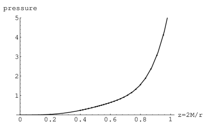
Figure 1: This graph shows the transverse pressure in the Unruh vacuum, both fitted and numerically estimated, as a function of $z=2M/r$ over the entire available data range.

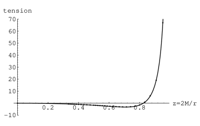
Figure 2: This graph shows the radial tension in the Unruh vacuum, both fitted and numerically estimated, as a function of $z=2M/r$, over the entire available data range.

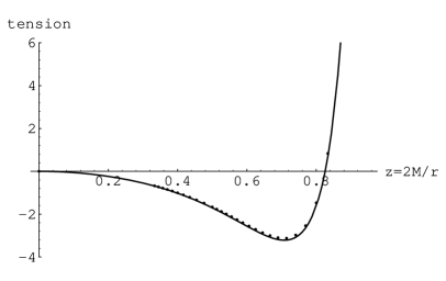
Figure 3: This graph shows the radial tension in the Unruh vacuum, both fitted and numerically estimated, as a function of $z=2M/r$, focussing on small $z$.

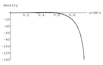
Figure 4: This graph shows the energy density in the Unruh vacuum, both fitted and numerically estimated, as a function of $z=2M/r$, over the entire available data range.

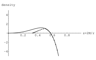
Figure 5: This graph shows the energy density in the Unruh vacuum, both fitted and numerically estimated, as a function of $z=2M/r$, focussing on small $z$. Note the discrepancy in the region below $z=0.5$, $r>4M$. (See footnote [27].)

There is an important consistency check that the semi-analytic model should pass: Elster has calculated [16] the total luminosity of a black hole against scalar emission using standard techniques [28] which are totally orthogonal to the present analysis. At each frequency he calculates a transmission coefficient which describes how much of the radiation leaving the event horizon actually makes it out to spatial infinity. [In (3+1) dimensions some radiation is always back-scattered from the gravitational field.] After multiplying this transmission coefficient by a Planckian spectrum and integrating over all frequencies Elster reports the total scalar luminosity as

$$L_{Elster}=7.44\times 10^{-5}M^{-2}.$$ (74)

In the notation of this paper, this translates to

$$f_{Elster}={81\over 16}{7.44\over 6.9941}\;p_{\infty}=5.385\;p_{\infty}.$$ (75)

On the other hand, the semi-analytic model gives

$$f_{0}=\left({96\over 20}+{59.0214\over 24}-{38.2068\over 20}\right)\;p_{\infty}=5.349\;p_{\infty}$$ (76)

That two such rather different techniques give total luminosities in such good agreement (better that $0.7\%$) is not only very encouraging, but is in fact a powerful consistency check on the numeric data. This completes construction of the semi-analytic model.

2.8 Matyjasek’s analysis

To compare my model to the model developed by Matyjasek [17] we should first note that Matyjasek does not base his model on the general Christensen–Fulling analysis as outlined and developed above, but instead uses a less general ansatz based on the Brown–Ottewill approximation [12]. What he calls his $N=6$ ansatz is (as presented) internally inconsistent. It is incapable of simultaneously fitting the luminosity data and giving the right asymptotic behaviour at infinity.

More precisely, if we fix the correct asymptotic behaviour at spatial infinity, then the luminosity is not a free parameter in Matyjasek’s $N=6$ ansatz. His ansatz is equivalent to keeping $k_{4}$ a free variable and setting $k_{5}=+6$ and $k_{6}=-9$, in which case $F(0)=-2/5$ and $f_{0}=5p_{\infty}$. (This is close to but not equal to the geometric optics approximation $f_{geometric-optics}\equiv 81/16=5.0625\neq 5$; it is certainly not equal to Elster’s calculated value $f_{Elster}=5.385$.) This analysis also forces Matyjasek’s $b_{2}$ coefficient to be exactly $b_{2}=5$. (Matyjasek’s $T$ is my $p_{\infty}$.) With only one free parameter ($b_{4}$) the $N=6$ ansatz can at best give only qualitative agreement with the numeric data.

Matyjasek’s $N=7$ ansatz has enough free parameters to fit both the asymptotic behaviour of the stress-energy and leave the luminosity as a free variable. This model is equivalent to setting $k_{6}=-9$, $k_{5}=126-24f_{0}/p_{\infty}$, and $k_{4}=[p|_{z=1}+24f_{0}]/p_{\infty}-117$. So in this model $F(0)=-2f_{0}+(96/10)p_{\infty}$. Matyjasek’s $N=7$ model has only two free parameters, $f_{0}$ and $p|_{z=1}$, the flux and the transverse pressure on the horizon, which he fits to these two single pieces of data as calculated by Elster and Jensen–McLaughlin–Ottewill. Matyjasek’s analysis does not use any of the other numeric data in any quantitative manner. With only two free parameters the $N=7$ ansatz still gives only qualitative agreement with the numeric data.

In contrast, my model has three completely free parameters, $k_{4}$, $k_{5}$, and $k_{6}$. I perform a global unconstrained fit to the totality of the available data, and provide a quantitative statement on the quality of the fit ($1\%$ accuracy). Furthermore, I use Elster’s luminosity calculation as a consistency check rather than as input.

3 Energy conditions

Outside the event horizon, the null energy condition (NEC; $\langle T_{\hat{\mu}\hat{\nu}}k^{\hat{\mu}}k^{\hat{\nu}}\geq 0?$) can be completely analyzed by looking at three special cases: outgoing null vectors, ingoing null vectors, and transverse null vectors. The NEC reduces to the three constraints

$$\rho(r)-\tau(r)\pm 2f\geq 0?\qquad\rho(r)+p(r)\geq 0?$$ (77)

3.1 Numerical analysis using the semi-analytic model

Numerically, these conditions are best investigated visually, by inspection of the relevant graphs.

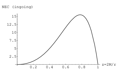
Figure 6: $\rho-\tau+2f$: This graph shows the NEC (evaluated using the semi-analytic model) on ingoing radial null vectors as a function of $z=2M/r$. Note that the curve is everywhere positive, so that the NEC is satisfied on ingoing null geodesics.

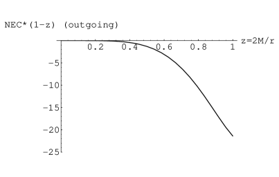
Figure 7: $\rho-\tau-2f$: This graph shows the NEC (evaluated using the semi-analytic model and multiplied by $(1-z)$ to control the singularity at the horizon) on outgoing radial null vectors as a function of $z=2M/r$. Note that the curve is everywhere negative, so that the NEC is violated on ingoing null geodesics.

Figure 8: $\rho-\tau-2f$: This graph shows the NEC (evaluated using the semi-analytic model, multiplied by $(1-z)$ to control the singularity at the horizon, and divided by $z^{5}$ to suppress the asymptotic behaviour at infinity) on outgoing radial null vectors as a function of $z=2M/r$. Note that the curve is everywhere negative, so that the NEC is violated on outgoing null geodesics.

Figure 9: $\rho+p$: This graph shows the NEC (evaluated using the semi-analytic model and multiplied by $(1-z)$ to control the singularity at the horizon) on transverse null vectors as a function of $z=2M/r$. Note that the curve changes sign near $z=0.6$. The NEC is satisfied on transverse null vectors far away from the black hole, and violated sufficiently near the black hole. (In particular the NEC is violated on the unstable photon orbit at $r=3M$.)

Figure 10: $\rho+p$: This graph shows the NEC (evaluated using the semi-analytic model, multiplied by $(1-z)$ to control the singularity at the horizon, and divided by $z^{2}$ to suppress the asymptotic behaviour at infinity) on transverse null vectors as a function of $z=2M/r$. Note that the curve changes sign near $z=0.6$. The NEC is satisfied on transverse null vectors far away from the black hole, and violated sufficiently near the black hole. (In particular the NEC is violated on the unstable photon orbit at $r=3M$.)

The fact that $\rho-\tau-2f$ is negative over the entire range $z\in[0,1]$, is enough to imply that at least in the outgoing radial direction the NEC is violated throughout the region exterior to the event horizon. Ipso facto all the pointwise energy conditions (null, weak, strong, and dominant) are violated throughout the entire region outside the event horizon, all the way to spatial infinity.

The pointwise energy conditions are violated in the sense that at every point outside the event horizon there is at least one null or timelike vector violating the conditions. It is certainly not true that all null or timelike vectors violate the energy conditions, nor is it true that the energy condition violations are large. What is true is that the violations are widespread.

Furthermore, this implies that the averaged null energy condition (ANEC) is violated on outgoing radial null geodesics. (More precisely, the one-sided ANEC that is cut off at the event horizon is violated). This automatically implies violations of (one-sided) averaged weak (AWEC) and averaged strong (ASEC) energy conditions.

One can also immediately see that the null energy condition is violated along the unstable photon orbit at $r=3M$ ($z=2/3$).

We could now add more detailed analyses of exactly which energy condition is violated where, along the lines reference [8], but the limited additional insight to be gained does not seem to warrant it.

3.2 Some analytic results

In the outgoing null direction we have the exact result [cf. eq. (42)]

$$\langle U|T^{\hat{\mu}\hat{\nu}}|U\rangle\;\ell^{+}_{\hat{\mu}}\ell^{+}_{\hat{\nu}} = \rho-\tau-2f,$$ (78)

$$= -4{z^{2}\over 1-z}\left[{F(z)-F(0)\over 2}+\xi\left({z^{4}\over 4}-{z^{5}\over 5}\right)\right].$$

But I have already shown [cf. eq. (52) and the discussion on p. 2.6] that $F(z)=F(0)+O(z^{3})$. Therefore, as previously asserted

$$\langle U|T^{\hat{\mu}\hat{\nu}}|U\rangle\;\ell^{+}_{\hat{\mu}}\ell^{+}_{\hat{\nu}}=O(z^{5}).$$ (79)

In fact, from eq. (52) we have $F(z)=F(0)+z^{3}Q_{1}(z)$, with $Q_{1}(z)$ having a power series that starts off with a constant $z^{0}$ term. Thus

$$\langle U|T^{\hat{\mu}\hat{\nu}}|U\rangle\;\ell^{+}_{\hat{\mu}}\ell^{+}_{\hat{\nu}}=-4{z^{5}\over 1-z}\left[{Q_{1}(z)\over 2}+\xi\left({z\over 4}-{z^{2}\over 5}\right)\right].$$ (80)

It is this explicit prefactor of $z^{5}/(1-z)$ that is responsible for most of the structure as seen in figures 7 and 8.

On the other hand, in the ingoing null direction it is easy to obtain the general result

$$\langle U|T^{\hat{\mu}\hat{\nu}}|U\rangle\;\ell^{-}_{\hat{\mu}}\ell^{-}_{\hat{\nu}} = \rho-\tau+2f,$$

$$= +{\xi\over 5}\;p_{\infty}z^{2}(1+z+z^{2}+z^{3}-4z^{4})-2{z^{2}\over 1-z}F(z),$$

$$= +{\xi\over 5}\;p_{\infty}\;z^{2}(1-z)(1+2z+3z^{2}+4z^{3})-2{z^{2}\over 1-z}F(z).$$

But from eq. (52) we know that $F(z)$ contains an explicit factor of $(1-z)^{2}$ so that $F(z)=(1-z)^{2}Q_{2}(z)$ with $Q_{2}(z)$ having a power series that starts off with a constant $z^{0}$ term. Thus

$$\langle U|T^{\hat{\mu}\hat{\nu}}|U\rangle\;\ell^{-}_{\hat{\mu}}\ell^{-}_{\hat{\nu}}=z^{2}(1-z)\left[{\xi\over 5}\;p_{\infty}(1+2z+3z^{2}+4z^{3})-2Q_{2}(z)\right].$$ (83)

It is this explicit prefactor of $z^{2}(1-z)$ that is responsible for most of the structure as seen in figure 6.

Finally, in the transverse direction one has the general result

$$\langle U|T^{\hat{\mu}\hat{\nu}}|U\rangle\;\ell^{\perp}_{\hat{\mu}}\ell^{\perp}_{\hat{\nu}} = \rho+p,$$ (85)

$$= -f_{0}{z^{2}\over 1-z}+{\xi\over 10}\;p_{\infty}z^{2}(1+z+z^{2}+z^{3}-9z^{4})$$

$$\qquad+2p(z)-2{z^{2}\over 1-z}F(z),$$

$$= {z^{2}\over 1-z}\Bigg{\{}-f_{0}+{\xi\over 10}\;p_{\infty}\;(1-z)(1+2z+3z^{2}-9z^{3})$$

$$\qquad+2(1-z){p(z)\over z^{2}}-2F(z)\Bigg{\}}.$$

But $p(z)=z^{4}Q_{3}(z)$ where $Q_{3}(z)$ has a power series that starts off with a constant $z^{0}$ term. Thus

$$\langle U|T^{\hat{\mu}\hat{\nu}}|U\rangle\;\ell^{\perp}_{\hat{\mu}}\ell^{\perp}_{\hat{\nu}} = {z^{2}\over(1-z)}\Big{[}-f_{0}+{\xi\over 10}\;p_{\infty}(1-10z^{4}-9z^{5})$$ (86)

$$\qquad+2(1-z)z^{2}Q_{3}(z)-2F(z)\Big{]}.$$

It is this explicit prefactor of $z^{2}/(1-z)$ that is responsible for most of the structure as seen in figures 9 and 10.

3.3 Some explicit results for the three-term model

This generic behaviour can easily be checked analytically for the simple three-term model developed in this paper. A little brute force yields

$$\rho-\tau+2f = p_{\infty}z^{2}(1-z)\Bigg{[}4\left({\xi\over 20}-{k_{5}\over 24}-{k_{6}\over 20}\right)+\left({2\xi\over 5}-{k_{5}\over 3}-{2k_{6}\over 5}\right)z$$ (87)

$$\qquad+\left({3\xi\over 5}-{k_{5}\over 2}-{3k_{6}\over 5}\right)z^{2}+\left({4\xi\over 5}-{4k_{6}\over 5}\right)z^{3}\Bigg{]}.$$

$$\rho-\tau-2f = p_{\infty}{z^{5}\over 1-z}\Bigg{[}{2k_{5}\over 3}-\left(\xi+{k_{5}\over 2}-k_{6}\right)z+\left({4\xi\over 5}-{4k_{6}\over 5}\right)\Bigg{]}.$$ (88)

$$\rho+p = p_{\infty}{z^{2}\over 1-z}\Bigg{[}\left({\xi\over 20}-{k_{5}\over 24}-{k_{6}\over 20}\right)+2k_{4}z^{2}+\left(-2k_{4}-{7k_{5}\over 3}\right)z^{3}$$ (89)

$$\qquad-\left(\xi+{9k_{5}\over 4}-{5k_{6}\over 2}\right)z^{4}+\left({9\xi\over 10}-{12k_{6}\over 5}\right)z^{5}\Bigg{]}.$$

The known analytic behaviour of the prefactors in these expressions serves as a consistency check on the numerical analysis used to generate the figures.

4 Discussion

In summary, in this paper I have developed a systematic way of building semi-analytic models for the stress-energy tensor in Schwarzschild spacetime. For the Unruh vacuum I have carried the program forward to the extent of explicitly deriving a three-parameter approximation to the total stress-energy that successfully fits all known data to better than $1\%$ accuracy. The model passes the consistency test of correctly predicting the luminosity from the fit to the transverse pressure.

In two appendices I sketch how this program can be extended to the Hartle–Hawking and Boulware states.

A central result of this paper is the observation that violations of the energy conditions, both pointwise and averaged, are ubiquitous (though small) in the Unruh vacuum. This $(3+1)$–dimensional result is qualitatively in agreement with the $(1+1)$–dimensional analytic model considered in [10]. Furthermore in view of the results quoted in [8, 9] we know that this is not a peculiarity of the Unruh vacuum, but that energy condition violations are also widespread in the Hartle–Hawking and Boulware vacuum states.

Note that I am claiming that the violations are widespread—I am not claiming they are large. These are intrinsically quantum mechanical effects with the typical scale of the effect near the horizon being given by

$$\langle T^{\hat{\mu}\hat{\nu}}\rangle\approx{\hbar c^{9}\over(GM)^{4}}.$$ (90)

Ford and Roman have argued [29, 30, 31] that in many situations the quantum inequalities may be of more interest than the energy conditions themselves. It seems that even if the energy condition violations are widespread, the quantum inequalities may more stringently constrain the dynamics [31]. The semi-analytic model developed in this paper may be of some interest in explicitly testing the quantum inequalities. (The analysis of this paper is fully consistent with qualitative features of the Ford-Roman results of [30], but the semi-analytic model of this paper will allow one to evaluate the relevant integrals more accurately. Note that although the coefficients were fitted using data from outside the event horizon there is nothing to stop us from taking the resulting model and applying it inside the event horizon.)

Finally, I remind the reader that issues of quantum mechanical violation of the energy conditions are of central importance to any attempt at taking the classical collapse theorems [22], the classical topological censorship theorem [32], or the classical positive mass theorem [33] and trying to see whether or to what extent these classical theorems can be generalized into the semiclassical world.

Appendix A Model building: Hartle–Hawking vacuum

There is nothing particularly sacred about the Unruh vacuum when it comes to model-building of the type discussed in this paper. Similar procedures can be applied in the Hartle–Hawking vacuum as well. This sort of modeling allows us to get a better handle on the underlying rationale behind the Page approximation—this approximation is in some sense (to be described below) the minimal form of the stress-energy tensor compatible with regularity on the horizon and a “thermal-bath plus curvature-corrections” ansatz at spatial infinity.

A.1 General analysis

For general background information see [18]. First, since the Hartle–Hawking vacuum is to be regular on the both the future horizon and past horizon we must have $f_{+}\equiv 0\equiv f_{-}$. (And hence the flux is identically zero: $f(z)\equiv 0$.) At asymptotic spatial infinity we want the stress-energy to look like that of an thermal bath of radiation at the Hawking temperature [18]. That is: we need to have $p(z)\to p_{\infty}$ asymptotically as $z\to 0$, while $\rho(z)\to 3p_{\infty}$, and $\tau(z)\to-p_{\infty}$. (For higher-spin fields $\rho(z)\to 3gp_{\infty}$, $\tau(z)\to-gp_{\infty}$, and $p(z)\to+gp_{\infty}$, with $g$ being the appropriate statistical weight.)

Substituting the result for $f_{0}$ back into the general expression for the stress-energy, the various components are seen to be

$$\rho(z) = +{\xi\over 10}\;p_{\infty}\;z^{2}\left(1+z+z^{2}+z^{3}-9z^{4}\right)+p(z)-{z^{2}\over 1-z}F(z).$$ (91)

$$\tau(z) = -{\xi\over 10}\;p_{\infty}\;z^{2}\left(1+z+z^{2}+z^{3}+z^{4}\right)+p(z)+{z^{2}\over 1-z}F(z).$$ (92)

The transverse pressure is still well-behaved all the way down to the horizon, so it still makes sense to look for a convergent power-series. But because of the known asymptotic behaviour, it is more useful to introduce four new parameters ($k_{0}$,$k_{1}$,$k_{2}$,and $k_{3}$; not present for the Unruh vacuum) and write:

$$p(z)\equiv p_{\infty}\;\sum_{n=0}^{\infty}k_{n}z^{n}.$$ (93)

A brief calculation yields

$$F(z) = +p_{\infty}\Bigg{\{}-2k_{0}{(1-z)^{2}\over z^{2}}-3k_{1}{1-z\over z}+2k_{2}(1-z)-k_{3}{(1-z)^{2}\over 2}$$

$$-(3k_{1}-2k_{2})\ln(z)$$

$$+(1-z)\left[\sum_{n=5}^{\infty}{(n-4)k_{n}\over(n-2)(n-1)}\left[1+z+z^{2}+\cdots+z^{n-3}-(n-2)z^{n-2}\right]\right]\Bigg{\}}.$$

Here I have kept the first few terms separate for clarity. Note that $k_{4}$ does not contribute to $F(z)$.

We are really only interested in the quantity

$${z^{2}\over 1-z}F(z) = +p_{\infty}\Bigg{\{}{-2k_{0}(1-z)}-3k_{1}z+2k_{2}z^{2}-k_{3}{z^{2}(1-z)\over 2}$$

$$-(3k_{1}-2k_{2}){z^{2}\ln(z)\over 1-z}$$

$$+z^{2}\left[\sum_{n=5}^{\infty}{(n-4)k_{n}\over(n-2)(n-1)}\left[1+z+z^{2}+\cdots+z^{n-3}-(n-2)z^{n-2}\right]\right]\Bigg{\}}$$

$$= +p_{\infty}\Bigg{\{}{-2k_{0}(1-z)}-3k_{1}z+2k_{2}z^{2}-k_{3}{z^{2}(1-z)\over 2}$$

$$-(3k_{1}-2k_{2}){z^{2}\ln(z)\over 1-z}+z^{2}\left[\sum_{n=5}^{\infty}{(n-4)k_{n}\over(n-2)(n-1)}\right]$$

$$+z^{3}\left[\sum_{n=5}^{\infty}{(n-4)k_{n}\over(n-2)(n-1)}\left[1+z+z^{2}+\cdots+z^{n-4}-(n-2)z^{n-3}\right]\right]\Bigg{\}}.$$

Which can now be substituted into the stress-energy to show

$$\rho(z) = p_{\infty}\Bigg{\{}+{\xi\over 10}\;z^{2}\left(1+z+z^{2}+z^{3}-9z^{4}\right)$$ (96)

$$\qquad+k_{0}(3-2z)+4k_{1}z-k_{2}z^{2}+k_{3}{z^{2}(1+z)\over 2}$$

$$\qquad+(3k_{1}-2k_{2}){z^{2}\ln(z)\over 1-z}-z^{2}\left[\sum_{n=5}^{\infty}{(n-4)k_{n}\over(n-2)(n-1)}\right]+\sum_{n=4}^{\infty}k_{n}z^{n}$$

$$\qquad-z^{3}\sum_{n=5}^{\infty}{(n-4)k_{n}\over(n-2)(n-1)}\left[1+z+z^{2}+\cdots+z^{n-4}-(n-2)z^{n-3}\right]\Bigg{\}},$$

$$\tau(z) = p_{\infty}\Bigg{\{}-{\xi\over 10}\;z^{2}\left(1+z+z^{2}+z^{3}+z^{4}\right)$$

$$\qquad-k_{0}(1-2z)-2k_{1}z+3k_{2}z^{2}-k_{3}{z^{2}(1-3z)\over 2}$$

$$\qquad-(3k_{1}-2k_{2}){z^{2}\ln(z)\over 1-z}+z^{2}\left[\sum_{n=5}^{\infty}{(n-4)k_{n}\over(n-2)(n-1)}\right]+\sum_{n=4}^{\infty}k_{n}z^{n}$$

$$\qquad+z^{3}\sum_{n=5}^{\infty}{(n-4)k_{n}\over(n-2)(n-1)}\left[1+z+z^{2}+\cdots+z^{n-4}-(n-2)z^{n-3}\right]\Bigg{\}}.$$

From the preceding analysis it is clear that this model satisfies all the known properties of the stress-energy tensor in the Hartle–Hawking vacuum (anomalous trace, covariant conservation, asymptotic behaviour both at spatial infinity and the horizon). Consequently these equations provide a general formalism for the stress-energy tensor in the Hartle–Hawking vacuum.

At first glance the presence of the logarithmic terms may be disturbing. Note that the logarithms show up only in the combination $S(z)\equiv[z^{2}\ln(z)]/(1-z)$. This combination remains finite both at the horizon ($\lim_{z\to 1}S(z)=-1$) and at spatial infinity ($\lim_{z\to 0}S(z)=0$), so the logarithmic terms should not be excluded a priori.

There is however a popular ansatz that justifies eliminating the logarithmic terms. Near spatial infinity we expect the stress-energy tensor to be that of a red-shifted thermal bath of radiation with curvature corrections. Schematically:

$$\langle H|T^{\hat{\mu}\hat{\nu}}|H\rangle(z)={\langle H|T^{\hat{\mu}\hat{\nu}}|H\rangle|_{\infty}\over(1-z)^{2}}+\hbox{``curvature-corrections''}?$$ (98)

Two versions of this ansatz will now be used to more precisely fix the form of the stress tensor.

A.2 Weak thermal bath ansatz

Since the curvature is proportional to $M/r^{3}$, we expect the “curvature corrections” to be (at worst) of order $z^{3}$, in which case we have the conservative ansatz:

$$\langle H|T^{\hat{\mu}\hat{\nu}}|H\rangle|_{z}=\langle H|T^{\hat{\mu}\hat{\nu}}|H\rangle|_{\infty}\left(1+2z+3z^{2}\right)+O(z^{3})?$$ (99)

If we adopt this ansatz, it enforces very specific choices on the first few coefficients. In fact, by looking at $p(z)$ it is trivial to see that $k_{0}=1g$, and $k_{1}=2g$, while $k_{2}=3g$. (Here $g$ is the statistical weight, $g=1$ for scalars. Also, remember to use the appropriate value of $\xi$ for higher spin.) This is enough to make the coefficients in front of the logarithmic terms vanish. It is easy to see that the $O(1)$ pieces of $\rho(z)$ and $\tau(z)$ are $3g$ and $-g$ respectively, while the $O(z)$ terms are $6g$ and $-2g$ respectively. Additionally, the $O(z^{2})$ pieces of $\rho(z)$ and $\tau(z)$ are proportional to

$${\xi\over 10}-3g+{k_{3}\over 2}-\sum_{n=5}^{\infty}{(n-4)k_{n}\over(n-2)(n-1)}=3\times 3g?$$ (100)

and

$$-{\xi\over 10}+9g-{k_{3}\over 2}+\sum_{n=5}^{\infty}{(n-4)k_{n}\over(n-2)(n-1)}=-3g?$$ (101)

respectively. So the conservative ansatz (99) can be simultaneously satisfied for all components of the stress-energy provided we pick

$$k_{3}=2\left[12g-{\xi\over 10}+\sum_{n=5}^{\infty}{(n-4)k_{n}\over(n-2)(n-1)}\right].$$ (102)

Note that with this choice of coefficients, not only do we satisfy the ansatz given above, but we also guarantee that the stress-energy tensor will agree with Page’s analytic approximation [11, 8] at least to order $O(z^{3})$. With this ansatz in place

$$p(z)\equiv p_{\infty}\;\left[g(1+2z+3z^{2})+k_{3}z^{3}+\sum_{n=4}^{\infty}k_{n}z^{n}\right].$$ (103)

The other components of the stress-energy tensor reduce to

$$\rho(z) = p_{\infty}\Bigg{\{}+3g(1+2z+3z^{2})+k_{3}{z^{3}\over 2}+{\xi\over 10}z^{3}(1+z+z^{2}-9z^{3})+\sum_{n=4}^{\infty}k_{n}z^{n}$$

$$\qquad-z^{3}\sum_{n=5}^{\infty}{(n-4)k_{n}\over(n-2)(n-1)}\left(1+z+z^{2}+\cdots+z^{n-4}-(n-2)z^{n-3}\right)\Bigg{\}},$$

$$\tau(z) = p_{\infty}\Bigg{\{}-g(1+2z+3z^{2})+k_{3}{3z^{3}\over 2}-{\xi\over 10}z^{3}(1+z+z^{2}+z^{3})+\sum_{n=4}^{\infty}k_{n}z^{n}$$

$$\qquad+z^{3}\sum_{n=5}^{\infty}{(n-4)k_{n}\over(n-2)(n-1)}\left(1+z+z^{2}+\cdots+z^{n-4}-(n+2)z^{n-3}\right)\Bigg{\}}.$$

This completes the weak ansatz. Note that $k_{3}$ is not a free variable and that it is $k_{4}$ and higher order coefficients that uniquely fix the stress tensor.

A.3 Strong thermal bath ansatz

A more radical ansatz is to assert that the “curvature-corrections” to the stress-energy tensor should be of asymptotic order $(curvature)^{2}$, that is of asymptotic order $z^{6}$. In this case we assert

$$\langle H|T^{\hat{\mu}\hat{\nu}}|H\rangle|_{z}=\langle H|T^{\hat{\mu}\hat{\nu}}|H\rangle|_{\infty}\left(1+2z+3z^{2}+4z^{3}+5z^{4}+6z^{5}\right)+O(z^{6})?$$ (106)

We should note in particular that the Page approximation satisfies this more radical ansatz. By considering $p(z)$ we automatically deduce $k_{0}=1g$, $k_{1}=2g$, $k_{2}=3g$, $k_{3}=4g$, $k_{4}=5g$, and $k_{5}=6g$, with $k_{6}$ and higher being left free by this ansatz. Instead of using brute force it is useful to first consider a subsidiary ansatz for $p(z)$:

$$p(z)=p_{\infty}\;g(1+2z+3z^{2}+4z^{3}+5z^{4}+6z^{5}+k_{6}).$$ (107)

It is now straightforward to compute

$${z^{2}\over 1-z}F(z) = p_{\infty}\;g\Big{[}(-2-4z+4z^{2}+2z^{3})+{1\over 2}z^{2}(1+z+z^{2}-3z^{2})$$ (108)

$$\qquad+{k_{6}\over 10}z^{2}(1+z+z^{2}+z^{3}-4z^{3})\Big{]}.$$

Inserting this into the stress-energy tensor

$$\rho = \rho_{\infty}\;g\Big{\{}(1+2z+3z^{2}+4z^{3}+5z^{4}+6z^{5}+k_{6})+(+2+4z-4z^{2}-2z^{3})$$ (109)

$$\qquad-{1\over 2}z^{2}(1+z+z^{2}-3z^{2})-{k_{6}\over 10}z^{2}(1+z+z^{2}+z^{3}-4z^{3})$$

$$\qquad+{(\xi/g)\over 10}z^{2}(1+z+z^{2}+z^{3}-9z^{2})\Big{\}}.$$

Collecting terms

$$\rho = \rho_{\infty}\;g\Bigg{\{}3+6z+z^{2}\left(-1+{(\xi/g)-k_{6}-5\over 10}\right)+z^{3}\left(+2+{(\xi/g)-k_{6}-5\over 10}\right)$$ (110)

$$\qquad+z^{4}\left(+5+{(\xi/g)-k_{6}-5\over 10}\right)+z^{5}\left(+8+{(\xi/g)-k_{6}-5\over 10}\right)$$

$$\qquad+z^{6}\left({14k_{6}-9(\xi/g)\over 10}\right)\Bigg{\}}.$$

This can be made to satisfy the strong thermal bath ansatz above if we pick $(\xi/g)-k_{6}-5=100$, that is

$$k_{6}={\xi\over g}-105.$$ (111)

Once we do this

$$p = p_{\infty}g\left\{(1+2z+3z^{2}+4z^{3}+5z^{4}+6z^{5})+\left({\xi\over g}-105\right)\right\}.$$ (112)

$$\rho = p_{\infty}g\left\{3(1+2z+3z^{2}+4z^{3}+5z^{4}+6z^{5})+\left({\xi\over 2g}-147\right)\right\}.$$ (113)

$$\tau = p_{\infty}g\left\{-(1+2z+3z^{2}+4z^{3}+5z^{4}+6z^{5})+\left({\xi\over 2g}-63\right)\right\}.$$ (114)

(The computation for $\tau$ is completely analogous to that just performed for $\rho$.) This is exactly Page’s analytic approximation [11, 8].

What does this computation tell us? If we take the strong ansatz, (that the stress-energy is a red-shifted thermal bath with curvature corrections of order $z^{6}$), and supplement this with the requirement that there be no terms of order higher than $z^{6}$, the we are led uniquely to the Page approximation for the stress-energy tensor surrounding a black hole. That is, the Page approximation is (in the sense described above) the minimal ansatz compatible with general properties of the stress-energy tensor.

Of course the Page approximation is not exact, and the stress-energy around Schwarzschild black holes does have some higher order contributions. Can we say anything about $O(z^{7})$ terms and higher? Indeed yes, when adding $O(z^{7})$ terms and higher to $p(z)$ we should be careful to not destroy the thermal bath ansatz for lower order terms. Suppose we write

$$p(z)=p_{Page}(z)+\delta p(z).$$ (115)

Then we have

$$\rho(z) = \rho_{Page}(z)-{z^{2}\over 1-z}\delta F(z).$$ (116)

$$\tau(z) = \tau_{Page}(z)+{z^{2}\over 1-z}\delta F(z).$$ (117)

So as to not destroy the strong thermal bath ansatz we need both $\delta p(z)=O(z^{6})$ or higher and $\delta F(z)=O(z^{4})$ or higher. We have already seen that we cannot possibly achieve this with any monomial in $z$. The best we can hope for is to find some suitable binomial such as

$$\delta p_{n}(z)=z^{n}-\epsilon_{n}z^{n+1}.$$ (118)

In which case

$$\delta F_{n}(z) = (1-z)\Bigg{\{}{(n-4)\over(n-2)(n-1)}\left[1+z+z^{2}+\cdots+z^{n-3}-(n-2)z^{n-2}\right]$$ (119)

$$\qquad-\epsilon_{n}{(n-3)\over(n-1)n}\left[1+z+z^{2}+\cdots+z^{n-2}-(n-1)z^{n-1}\right]\Bigg{\}}$$

So if we pick $\epsilon_{n}=[n(n-4)]/[(n-2)(n-3)]$ there are massive cancellations and

$$\delta F_{n}(z)=-{n-4\over n-2}z^{n-2}(1-z)^{2}.$$ (120)

That is to say

$${z^{2}\over 1-z}\delta F_{n}(z)=-{n-4\over n-2}z^{n}(1-z).$$ (121)

Consequently the binomials

$$\delta p(z)=z^{n}-{n(n-4)\over(n-2)(n-3)}z^{n+1}$$ (122)

(for $n\geq 6$) are a useful “basis” for the pieces of the stress-energy tensor that go beyond the Page approximation. These basis elements are useful in the sense that they do not perturb the lower order pieces of the stress-energy.

I shall report elsewhere the results of performing such fits to the Anderson–Hiscock–Samuel data.

Appendix B Model building: Boulware vacuum

Unsurprisingly, a similar analysis can be applied in the Boulware vacuum. Again, for general background information see [18]. First, since there is no net flow of radiation in the Boulware vacuum we must have $f_{+}\equiv f_{0}\equiv f_{-}$. (And hence $f(z)=0$). At asymptotic spatial infinity we want the stress-energy to be as small as possible. Since if nothing else the anomaly will generate terms of order $O(z^{6})$, Christensen and Fulling were led to tentatively suggest $\langle H|T^{\hat{\mu}\hat{\nu}}|H\rangle=O(z^{6})$ [18, page 2096].

To at least force the terms of order $O(z^{2})$ to vanish we need to enforce

$${\xi\over 10}+G(0)+2f_{0}=0.$$ (123)

That is

$$f_{0}=-{\xi\over 20}\;p_{\infty}-{G(0)\over 2}.$$ (124)

(This is formally very similar to what we found for the Unruh vacuum, up to a few critical minus signs.) Substituting this result for $f_{0}$ back into the general expression for the stress-energy, the various components are seen to be

$$\rho(z) = -{\xi\over 10}\;p_{\infty}\;z^{6}{10-9z\over 1-z}+2p(z)+{z^{2}\over 1-z}\left[G(z)-G(0)\right].$$ (125)

$$\tau(z) = +{\xi\over 10}\;p_{\infty}\;{z^{7}\over 1-z}-{z^{2}\over 1-z}\left[G(z)-G(0)\right].$$ (126)

I have actually pulled a minor swindle to get to this point because $G(0)$, $G(z)$, and $f_{0}$ are all ill-defined infinite quantities in the Boulware vacuum. This happens because $p(z)$ diverges at the horizon, and the integral used to define $G(z)$ does not converge. Fortunately this does not matter, since the final expression for the stress-energy contains only terms of the type

$$\bar{G}(z)\equiv\left[G(z)-G(0)\right]\equiv-\int_{0}^{z}\left({2\over{\bar{z}}^{3}}-{3\over{\bar{z}}^{2}}\right)\;p(\bar{z})\;d{\bar{z}}.$$ (127)

This integral converges provided $p(z)$ is of order $O(z^{3})$ or smaller at spatial infinity. The divergence at the horizon does not matter because the range of integration does not include the horizon.

We can further define

$$\bar{F}(z)\equiv\left[F(z)-F(0)\right]\equiv-\int_{0}^{z}{\bar{z}}^{2}\;(1-{\bar{z}})\;{d\over d\bar{z}}\left({p(\bar{z})\over{\bar{z}}^{4}}\right)\;d{\bar{z}}.$$ (128)

Then, integrating by parts, it is easy to show that

$$\bar{G}(z)=-{1-z\over z^{2}}p(z)-\bar{F}(z).$$ (129)

Doing this requires only the mild assumption that $p(z)$ is is of order $O(z^{3})$ or smaller at spatial infinity, which we already had to assume anyway.

The components of the stress-energy tensor can now be rewritten as

$$\rho(z) = -{\xi\over 10}\;p_{\infty}\;z^{6}{10-9z\over 1-z}+p(z)-{z^{2}\over 1-z}\bar{F}(z).$$ (130)

$$\tau(z) = +{\xi\over 10}\;p_{\infty}\;{z^{7}\over 1-z}+p(z)+{z^{2}\over 1-z}\bar{F}(z).$$ (131)

The transverse pressure is still well-behaved until you get to the horizon, so it still makes sense to look for a power-series; though now we expect this power series to have radius of convergence of one, and to diverge at the horizon. Because of the minimal $O(z^{3})$ asymptotic behaviour I have argued for above, it is instructive to write

$$p(z)\equiv p_{\infty}\;\left[k_{3}z^{3}+\sum_{n=4}^{\infty}k_{n}z^{n}\right].$$ (132)

A brief calculation yields

$$\bar{F}(z)=+p_{\infty}\left\{k_{3}\left(z-{z^{2}\over 2}\right)+\left[\sum_{n=5}^{\infty}(n-4)k_{n}\left({z^{n-1}\over n-1}-{z^{n-2}\over n-2}\right)\right]\right\}$$ (133)

Which can now be substituted into the stress-energy to show

$$\rho(z) = p_{\infty}\Bigg{\{}-{\xi\over 10}\;z^{6}{10-9z\over 1-z}-k_{3}{z^{4}\over 2(1-z)}+\sum_{n=4}^{\infty}k_{n}z^{n}$$ (134)

$$\qquad-{z^{2}\over 1-z}\sum_{n=5}^{\infty}(n-4)k_{n}\left({z^{n-1}\over n-1}-{z^{n-2}\over n-2}\right)\Bigg{\}},$$

$$\tau(z) = p_{\infty}\Bigg{\{}+{\xi\over 10}\;{z^{7}\over 1-z}+k_{3}{z^{3}(4-3z)\over 1-z}+\sum_{n=4}^{\infty}k_{n}z^{n}$$ (135)

$$\qquad+{z^{2}\over 1-z}\sum_{n=5}^{\infty}(n-4)k_{n}\left({z^{n-1}\over n-1}-{z^{n-2}\over n-2}\right)\Bigg{\}}.$$

We again see from the preceding analysis that this model satisfies all the known properties of the stress-energy tensor in the Boulware vacuum (anomalous trace, covariant conservation, asymptotic behaviour both at spatial infinity and the horizon). Consequently these equations provide a general formalism for the stress-energy tensor in the Boulware vacuum.

It is possible to improve the situation by making several simplifying ansatze. If we assume that all non-zero components of the stress-energy tensor should asymptotically be of the same order, then we must set $k_{3}=0$. If (following Christensen–Fulling) we make the stronger ansatz that that all non-zero components are of order $O(z^{6})$ one has $k_{3}=k_{4}=k_{5}=0$. In this case it is easy to check that

$$\rho(z) = p_{\infty}\;\left(-\xi+{3\over 2}\;k_{2}\right)z^{6}+O(z^{7}).$$ (136)

$$\tau(z) = p_{\infty}\;{1\over 2}\;k_{2}\;z^{6}+O(z^{7}).$$ (137)

$$p(z) = p_{\infty}\;k_{2}\;z^{6}+O(z^{7}).$$ (138)

For $k_{6}=-16$ this is compatible with the Brown–Ottewill analytic approximation [12]. I have not found any nice principle that would uniquely lead from this general decomposition to the full Page–Brown–Ottewill approximation.

Serious model building is now simply a matter of getting good enough data to make reasonable estimates of the various coefficients $k_{n}$. One might even hope that with a little more work it might prove easier to analytically calculate these coefficients in preference to the numerically intensive work required to calculate the stress-energy components directly.

References

- [*] Electronic mail: visser@kiwi.wustl.edu
- [1] B. S. DeWitt, Phys. Rep. 19, 295 (1975), see especially pp. 342–345.
- [2] General Relativity: An Einstein Centenary Survey, edited by S. W. Hawking and W. Israel (Cambridge University Press, Cambridge, England, 1979).
- [3] N. D. Birrell and P. C. W. Davies, Quantum Fields in Curved Space (Cambridge University Press, Cambridge, England, 1982).
- [4] 300 Years of Gravitation, edited by S. W. Hawking and W. Israel (Cambridge University Press, Cambridge, England, 1987).
- [5] S. A. Fulling, Aspects of Quantum Field Theory in Curved Space–Time (Cambridge University Press, Cambridge, England, 1989).
- [6] M. Visser, Lorentzian wormholes — from Einstein to Hawking (American Institute of Physics, New York, 1995).
- [7] M. Visser, Scale anomalies imply violation of the averaged null energy condition, Phys. Lett. B349, 443 (1995); gr-qc/9409043
- [8] M. Visser, Gravitational vacuum polarization I: Energy conditions in the Hartle–Hawking vacuum, Physical Review D54 (1996) 5103–5115; gr-qc/9604007.
- [9] M. Visser, Gravitational vacuum polarization II: Energy conditions in the Boulware vacuum, Physical Review D54 (1996) 5116–5122; gr-qc/9604008.
- [10] M. Visser, Gravitational vacuum polarization III: Energy conditions in the (1+1) Schwarzschild spacetime, Physical Review D54 (1996) 5123–5128; gr-qc/9604009.
- [11] D. N. Page, Phys. Rev. D 25, 1499 (1982).
- [12] M. R. Brown and A. C. Ottewill, Phys. Rev. D 31, 2514 (1985).
- [13] B. P. Jensen, J. G. McLaughlin, and A. C. Ottewill, Phys. Rev. D 43, 4142 (1991).
- [14] B. Jensen, Private communication.
- [15] A. Ottewill, Private communication.
- [16] T. Elster, Phys. Lett. 94 A, 205 (1983).
- [17] J. Matyjasek, Approximate stress tensor of massless scalar field for an evaporating black hole, Class. Quant. Grav. 14 L15–L20 (1997).
- [18] S. M. Christensen and S. A. Fulling, Phys. Rev. D 15, 2088 (1977).
- [19] C. W. Misner, K. S. Thorne, and J. A. Wheeler, Gravitation (W. H. Freeman and Company, San Francisco, 1973).
- [20] S. Weinberg, Gravitation and Cosmology (Wiley, New York, 1972).
- [21] R. M. Wald, General Relativity (University of Chicago Press, Chicago, 1984).
- [22] S.W. Hawking and G.F.R. Ellis, The large scale structure of space-time, (Cambridge,England,1973).
- [23] K. W. Howard, Phys. Rev. D 30, 2532 (1984).
- [24] In fact there are two minor problems with the scalar data of reference [13]. In figure 4 on page 4143 the difference data for the radial tension () is correctly plotted but has inadvertently been multiplied by an extraneous factor of one-half before being added to Howard’s estimate for the radial tension. That is: , or . A second minor problem with the energy density is discussed below.
- [25] P. R. Anderson, W. A. Hiscock, and D. A. Samuel, Phys. Rev. Lett. 70, 1739 (1993).
- [26] P. Anderson, Private communication.
- [27] In fact the semi-analytic model correctly reproduces the Jensen–McLaughlin–Ottewill data for the radial tension (once allowance for the extraneous factor of one-half has been made). The semi-analytic fit also reproduces the data for the energy density in the range , but exhibits small but systematic deviations (too large to simply be numerical slop) in the range . I attribute these deviations to a bug in the integration routine used by Jensen–McLaughlin–Ottewill to calculate their density data from their pressure data. As a check on this I have evaluated the anomalous trace using the Jensen–McLaughlin–Ottewill data and find that it in the range it does not equal , the difference being completely ascribable to this bug in their calculation of the energy density.
- [28] D. N. Page, Phys. Rev. D 13, 198 (1976).
- [29] L. H. Ford and T. A. Roman, Averaged energy conditions and quantum inequalities, Phys. Rev. D 51, 4277 (1995); gr-qc/9410043.
- [30] L. H. Ford and T. A. Roman, Averaged energy conditions and evaporating black holes, Phys. Rev. D53 1988-2000 (1996); gr-qc/9506052.
- [31] L. H. Ford and T. A. Roman, Quantum field theory constrains traversable wormhole geometries, Phys. Rev. D53 5496-5507 (1996); gr-qc/9510071.
- [32] J. L. Friedman, K. Schleich, and D. M. Witt, Phys. Rev. Lett. 71, 1486 (1993).
- [33] R. Penrose, R. D. Sorkin, and E. Woolgar, (1993), gr-qc/9301015.