Dualities, CPT Symmetry and Dimensional Reduction in String Theory

Abstract

In this lecture we address the following issues in the context of string theories: i) The role played by $S$ and $T$ dualities in obtaining topological inflation in N=1 supergravity models, ii) A mechanism to generate the baryon asymmetry of the Universe based on the string interactions that violate CPT symmetry and iii) The quantum cosmology of the dimensionally reduced multidimensional Einstein-Yang-Mills system.

1 INTRODUCTION

One of the most challenging aspects of string unification and its D-brane relatives is the non-trivial task of reconstructing our four-dimensional world in a consistent fashion. The most direct theoretical scenario one can envisage for this purpose is the one where the important ingredients required for explaning the main features of our Universe can be all directly derived from the fundamental theory. This implies that problems such as the initial singularity of classical theories of gravity, the cosmological constant problem and the issue of intital conditions of our Universe among many others can be all tackled by stringy and/or D-brane physics. The next scenario, and probably the simplest one from the technical point of view, is to assume that for dynamical reasons the fundamental theory has gone through a considerable dimensional reduction process and that solutions of the abovementioned difficulties are to be found in the field theory limit of those theories. Until fairly recently the question whether this limit was meaningful would prevent one considering seriously the latter possibility, however the conjecture that $S$-duality [1] is a symmetry of the fundamental theory gives this hypothesis a better grounding. Indeed, this symmetry sheds light on the physics of the non-perturbative regime and hence on its connection with the field theory limit. This implies that $S$-duality should, likewise the already well stablished $T$-duality [2], be introduced in the supergravity models arising from the fundamental theory. It is precisely in the context of these dual N=1 supergravity models that is shown the moduli fields can be stabilized and the dilaton runaway problem solved [1]. It is also in this context that inflationary models can be built, either assuming that the inflaton is a singlet of the gauge sector [3] or that inflation of the topological type occurs [4]. This particular issue is going to be discussed in the first part of this lecture.

In the second part of this lecture, we discuss how a sizeable baryon asymmetry of the Universe can be generated via CPT violating string interactions [5] arising from the non-trivial solutions of the field theory of open strings [6]. Finally, we close with a discussion on the quantum cosmology of the multidimensional Einstein-Yang-Mills system after suitable dimensional reduction [7]. We aim with this last discussion to illustrate the well known point that in order to obtain solutions of a given theory a set of initial conditions is required and that for this purpose quantum cosmology seems to be particularly suitable as it allows for an easy implementation of the relevant symmetries as well as for solving the associated dynamical contraints.

2 TOPOLOGICAL INFLATION IN DUAL STRING MODELS

Superstring unification seems to be particularly fit for constructing inflationary cosmological scenarios. The existence of numerous scalar fields, the moduli, would seem to provide a necessary ingredient, however the fact that these fields remain massless at all orders in string perturbation theory leads to difficulties in building a sucessful cosmological scenario. Among the many moduli, the dilaton ($\phi$), stands out as it controls the string coupling and variations of this field correspond to changes in masses and coupling constants which are strongly constrained by observation. This question is usually addressed by assuming the dilaton develops a potential due to non-perturbative effects, such as gaugino condensation, and in this way Einstein’s gravity can be recovered after $\phi$ settles into the minimum of its potential. However, general arguments show that the dilaton cannot be stabilized in the perturbative regime of string theory leading to a runaway problem [8]. Moreover, even if the dilaton were stabilized by non-perturbative potentials, these are in general too steep to be suitable for inflation without fine-tuning the initial conditions [9, 10]. Of course, once the dilaton is fixed, inflation can be achieved via other fields, e.g. chiral fields (gauge singlets) for a suitable choice of the inflationary sector of the superpotential [11, 12]. Furthermore, there are additional difficulties such as the Polonyi problem associated with scalar fields that couple only gravitationally and which may dominate the energy density of the Universe at present [13, 14, 15, 16, 17, 18, 19, 20, 21].

It is known that some of the abovementioned difficulties can be avoided imposing the requirement of $S$-duality as it is shown that the dilaton potential develops a suitable minimum in this case [1]. Already in Ref. [3] this mechanism was used to stabilise the dilaton while inflation was accomplished by chiral fields. However, our analysis shows that inflation can be achieved via the dilaton itself provided one considers a novel way of implementing the inflationary expansion of the Universe, namely topological or defect inflation. In this scenario [22, 23], one shows that the core of a topological defect may undergo exponential inflationary expansion provided the scale of symmetry breaking, $\xi$, satisfies the condition

$$\xi>{\cal O}(M_{P})~{}.$$ (1)

The ensued inflationary process is eternal since the core of the defect is topologically stable and it is the restored symmetry in the core that provides the vacuum energy for inflation. We show that the conditions for successful inflation are satisfied by domain walls that separate degenerate minima in $S$-dual superstring potentials [4].

$S$-duality was conjectured [1] in analogy with the well-established $T$-duality symmetry of string compactification [2]. It is shown that the effective supergravity action following from string compactification on orbifolds or even Calabi-Yau manifolds is constrained by an underlying string symmetry, the so-called target space modular invariance [24]. The target space modular group $PSL(2,Z)$ acts on the complex scalar field $T$ as

$$T\to{aT-ib\over icT+d}\qquad;a,b,c,d\in Z,ad-bc=1~{},$$ (2)

and $<T>$ is the background modulus associated to the overall scale of the internal six-dimensional space on which the string is compactified. Specifically, $T=R^{2}+iB$, with $R$ being the “radius” of the internal space and $B$ an internal axion. The target space modular transformation contains the well-known duality transformation $R\to 1/R$ as well as discrete shifts of the axionic background $B$ [2]. Furthermore, this symmetry is shown to remain unbroken at any order of string perturbation theory. The conjectured $S$-duality symmetry would be a further modular invariance symmetry in string theory, where the modular group now acts on the complex scalar field $S=\phi+i\chi$, and $\chi$ is a pseudoscalar (axion) field. This symmetry includes a duality invariance under which the dilaton gets inverted. $S$-modular invariance strongly constrains the theory since it relates the weak and strong coupling regimes as well as the “$\chi$-sectors” of the theory.

The form of the N=1 supergravity action including gauge and matter fields is specified by the functions $G(\Phi,\Phi^{*})=K(\Phi,\Phi^{*})+\ln|W(\Phi)|^{2}$ and $f(\Phi)$; $K(\Phi,\Phi^{*})$ is the Kähler potential, $W(\Phi)$ the superpotential and $f(\Phi)$ the coupling among chiral matter fields, generically denoted by $\Phi$, and the kinetic terms of gauge fields. At string tree-level, the Kälher potential is given in terms of the chiral fields $S,\ T$ by

$$K=-\ln(S+S^{*})-3\ln(T+T^{*})~{}.$$ (3)

The scalar potential can be then written in the following form [1]

$$V=|h^{S}|^{2}G_{SS^{*}}^{-1}+|h^{T}|^{2}G_{TT^{*}}^{-1}-3\exp(G)~{},$$ (4)

where $h^{i}=\exp({\textstyle{{1}\over{2}}}G)G^{i}$, $i=S,T$ and the indices denote derivatives with respect to the indicated variable.

We look first at the case where there is only the $T$ modulus field. It is known that the purely $T$-dependent superpotential has to vanish order by order in perturbation theory so that the vacuum expectation value of $T$ remains undetermined. However, one expects that non-perturbative effects will generate a superpotential for $T$. The simplest expression for $W(T)$ compatible with modular invariance is [1]

$$W(T)\sim\eta(T)^{-6}$$ (5)

and the related scalar potential is given by [1]:

$$V(T)={1\over T_{R}^{3}|\eta(T)|^{12}}\left({T_{R}^{2}\over 4\pi^{2}}|\hat{G}_{2}(T)|^{2}-1\right),$$ (6)

where $T_{R}=2{\rm Re}\ T$. The function $\eta(T)=q^{1/24}\prod_{n}(1-q^{n})$ is the Dedekind function, $q=\exp(-2\pi T)$; $\hat{G}_{2}=G_{2}-2\pi/T_{R}$ is the weight two Eisenstein function and $G_{2}={\textstyle{{1}\over{3}}}\pi^{2}-8\pi^{2}\sigma_{1}(n)\exp(-2\pi nT)$, where $\sigma_{1}(n)$ is the sum of the divisors of $n$.

If, on the other hand, one considers only the $S$ field, the requirement of modular invariance associated with $S$-duality leads to the following scalar potential [1]

$$V(S)={1\over S_{R}|\eta(S)|^{4}}\left({S_{R}^{2}\over 4\pi^{2}}|\hat{G}_{2}(S)|^{2}-3\right).$$ (7)

This potential (like $V(T)$) diverges in the limits $S\to 0,\infty$ and has minima at finite values of $S$, close to the critical value $S=1$. Indeed, the function $\hat{G}_{2}(S)$ has its only zeros at $S=1,\ S=\exp({\textstyle{{1}\over{6}}}i\pi)$. The potential has other extrema, namely minima, for ${\rm Re}\ S\sim 0.8,\ 1.3$ and ${\rm Im}\ S=n,\ n\in Z$; these are minima both along the ${\rm Re}\ S$ and ${\rm Im}\ S$ directions. The qualitative shape of the potential is shown in Figure 1.

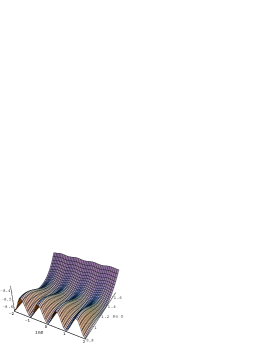
Figure 1:

Hence, the same way target space modular invariance fixes the value of $T_{R}$ forcing the theory to be compactified, $S$-modular invariance fixes the value of $S_{R}$ thus stabilizing the potential and avoiding the dilaton runaway problem. Furthermore, it is clear that the theory has to choose among an infinity of degenerate minima whose positions differ by modular transformations. Once one of them is chosen, target space modular invariance is spontaneously broken. Since duality is a discrete symmetry, if there were a phase in the evolution of the Universe in which the compactification radius was already chosen, $S$-duality domain walls would be created separating different vacua.

A more realistic model is obtained once all gauge singlet fields of the theory: $S,T_{i}$, $i=1,2,3$ are considered and $S$ and $T$ dualities are imposed on the $N=1$ supergravity Lagrangian [3]. A model of this type involves also untwisted chiral fields related to the $T_{1}$ sector. Assuming that the $T$-fields and the untwisted fields of the $T_{1}$ sector have already settled at the minimum of the potential and that inflation takes place due to the $S$-field, the relevant potential can be then written as [4]

$$V(S)={1\over S_{R}|\eta(S)|^{4}}\left({S_{R}^{2}\over 4\pi^{2}}|\hat{G}_{2}(S)|^{2}-a\right),$$ (8)

where $a$ is a constant. As for the models discussed above, we shall further assume that $S_{R}$ has settled at the minimum of the potential (at $<S_{R}>=2$) and inflation then takes place at the core of domain walls that separate different vacua, along the ${\rm Im}\ S$ direction.

In what follows it is shown that the conditions for topological inflation to occur at the core of the domain walls separating degenerate minima of the potential Eq. (8) can be met for a range of the parameter $a$.

Let us first discuss the conditions for successful topological inflation. Along a domain wall the field $\chi$ ranges from one minimum in one region of space to another minimum in another region. Somewhere between, $\chi$ must traverse the top of the potential, $\chi\approx\chi_{0}$, which can be expanded as

$$V\approx V_{0}\left(1-\alpha^{2}{(\chi-\chi_{0})^{2}\over M^{2}}\right),$$ (9)

where $\alpha^{2}$ is a constant and $M=M_{P}/\sqrt{8\pi}$, is the natural scale of the fields in supergravity (which has been set to one in the previous discussion).

In flat space, the wall thickness is equal to the curvature of the effective potential, that is $\delta^{-1}\sim\alpha(V_{0}/M_{P}^{2})^{1/2}$. The Hubble parameter in the interior of the wall is given by $H\approx(V_{0}/3M^{2})^{1/2}$. If $\delta\ll H^{-1}$, gravitational effects are negligible. However, if $\delta>H^{-1}$, the region of false vacuum near the top of the potential, $V\approx V_{0}$, extends over a region greater than a Hubble volume. Hence, if the top of the potential satisfies the conditions for inflation, the interior of the wall inflates. Demanding that $\delta>H^{-1}$, one obtains the following condition on $\alpha$,

$$\alpha^{2}<8\pi/3~{}.$$ (10)

However, the most stringent constraint on $\alpha$ arises for the requirement that there is at least $N_{e}$ e-folds of inflation (we assume here that $N_{e}=65$) [21]:

$$\alpha^{2}<3\pi/65~{}.$$ (11)

We have computed $\alpha^{2}$ for the purely $T$-dual and $S$-dual potentials, Eqs. (6) and (7), assuming that the real part of the $(T,\ S)$ field has already settled at the minimum of the potential. The envisaged scenario assumes that inflation takes place at the core of domain walls separating different vacua, as the imaginary part of the $(T,\ S)$ field expands exponentially once the conditions discussed above are satisfied at the top of potential. We find that $\alpha^{2}=0.30$ and $\alpha^{2}=0.09$, respectively; hence we conclude that the conditions for successful defect inflation to occur are fulfilled in the purely S-dual case only [4].

In the model with $S$ and $T$ dualities, the value of $\alpha^{2}$ depends on the constant $a$ (and therefore of vacuum contributions of the untwisted chiral fields, $|P|^{2}$ and $F_{0}$ as discussed in Ref. [4]). It is found that for $a\geq 2.5$ (this implies that $F_{0}<0$), successful topological inflation can occur in realistic models as well. We point out that the effect of the non-canonical struture of the kinetic terms of $S$ (and $T$) dictated by N=1 supergravity , $(S_{R})^{-2}\partial_{\mu}S\partial^{\mu}S^{*}$ $((T_{R})^{-2}\partial_{\mu}T\partial^{\mu}T^{*})$ has been considered and it does not affect our results due to the modular invariance.

Hence, we conclude that topological or defect inflation is possible for purely $S$-dual N=1 supergravity models and in $S$- and $T$-dual models where $a\geq 2.5$ (cf. Eq. (8)), thereby solving the cosmological initial condition problems of these models.

3 CPT VIOLATION AND BARYOGENESIS

Let us now discuss a mechanism for generating the baryon asymmetry of the Universe that involves a putative violation of the CPT symmetry arising from string interactions [5]. The usual conditions for baryogenesis, namely, violation of baryon number, violation of C and CP symmetries, and existence of nonequilibrium processes are well known [25]. These conditions can be met in a grand-unified theory (GUT) through the decay of heavy states at high energy [26, 27, 28, 29], through the decay of states in supersymmetric or superstring-inspired models at somewhat lower energies [30, 31, 32], or via the thermalization of the vacuum energy of supersymmetric states [33]. These conditions can also be satisfied in the electroweak theory through sphaleron-induced transitions between inequivalent vacua above the electroweak phase transition [34]. Spharelon-induced transitions can on the other hand dilute baryon asymmetries generated at higher energies [35].

Our mechanism is based on the observation that certain string theories may spontaneously break CPT symmetry [6]. If CPT and baryon number are violated, a baryon asymmetry could arise in thermal equilibrium [36, 37]. A mechanism for baryogenesis along these lines has the advantage of being independent of C- and CP-violating processes, which in GUTs are usually rather contrived to account for the observed baryon asymmetry and are unrelated to the experimentally observed CP violation in the standard model.

We assume that the source of baryon-number violation is due to processes mediated by heavy leptoquark bosons of mass $M_{X}$ in a generic GUT whose details play no essential role in our mechanism. Baryon-number violation in the early Universe from the leptoquarks is assumed to be negligible below some temperature $T_{D}$.

The CPT-violating interactions are shown to arise from the trilinear vertex of non-trivial solutions of the field theory of open strings and in the corresponding low-energy four-dimensional effective Lagrangian via couplings between Lorentz tensors $N$ and fermions $\varphi$, $\psi$ [6]. Suppressing Lorentz indices for simplicity, these have the schematic form $L\supset\lambda{M_{S}}^{-k}N\cdot\overline{\psi}\Gamma(i\partial)^{k}\varphi+h.c.$, where $\lambda$ is a dimensionless coupling constant, $M_{S}$ is a large mass scale (presumably close to the Planck mass), $\Gamma$ denotes a gamma-matrix structure, and $(i\partial)^{k}$ represents the action of a four-derivative at order $k\geq 0$. The CPT violation appears when appropriate components of $N$ acquire non-vanishing vacuum expectation values $\langle{N}\rangle$.

For simplicity, only the subset of the CPT-violating terms leading directly to a momentum- and spin-independent energy shift of particles relative to antiparticles are considered. Terms of this form can generate effects in neutral-meson systems that can be observed [6, 38]. These terms are diagonal in the fermion fields and involve expectation values of only the time components of $N$:

$$L={\lambda\langle{N}\rangle\over M_{S}^{k}}\overline{\psi}(\gamma^{0})^{k+1}(i\partial_{0})^{k}\psi+h.c.+...\quad.$$ (12)

Since no large CPT violation has been observed, the expectation value $\langle{N}\rangle$ must be suppressed in the low-energy effective theory. The suppression factor is presumably some non-negative power $l$ of the ratio of the low-energy scale $m_{l}$ to $M_{S}$, that is $\langle{N}\rangle\sim(m_{l}/M_{S})^{l}M_{S}$. Since each factor of $i\partial_{0}$ also acts to provide a low-energy suppression, the condition $k+l=2$ corresponds to the dominant terms [6]. In what follows, we consider the various values of $k$ and $l$ in turn.

For the baryogenesis scenario it is assumed that each fermion $\psi$ represents a standard-model quark of mass $m_{q}$ and baryon number $1/3$. The energy splitting between a quark and its antiquark arising from Eq. (12) can be viewed as an effective chemical potential, $\mu$, driving the production of baryon number in thermal equilibrium.

We consider a CPT-violating coupling for a single quark field. The equilibrium phase-space distributions of quarks $q$ and antiquarks $\bar{q}$ at temperature $T$ are $f_{q}(\vec{p})=(1+e^{(E-\mu)/T})^{-1}$ and $f_{\bar{q}}(\vec{p})=(1+e^{(E+\mu)/T})^{-1}$, respectively, where $\vec{p}$ is the momentum and $E=\sqrt{m_{q}^{2}+p^{2}}$. If $g$ is the number of internal quark degrees of freedom, then the difference between the number densities of quarks and antiquarks is

$$n_{q}-n_{\bar{q}} = {g\over(2\pi)^{3}}\int d^{3}p~{}[f_{q}(\vec{p})-f_{\bar{q}}(\vec{p})]\quad.$$ (13)

The contribution to the baryon-number asymmetry per comoving volume is given by $n_{B}/s\equiv(n_{q}-n_{\bar{q}})/s$, and on its turn the entropy density $s(T)$ of relativistic particles is given by

$$s(T)={2\pi^{2}\over 45}g_{s}(T)T^{3}\quad,$$ (14)

$$g_{s}(T)=\sum_{B}g_{B}\left(T_{B}\over T\right)^{3}+{7\over 8}\sum_{F}g_{F}\left(T_{F}\over T\right)^{3}~{},$$ (15)

where the number of degrees of freedom of relativistic bosons $B$ and fermions $F$ are taken to be $g_{B}$ and $g_{F}$, respectively, such that their component temperatures are denoted $T_{B}$ and $T_{F}$. Photon and quark gases have the same temperature $T$.

Considering initially the case $k=0$ with $l=2$, it follows from Eq. (12) that the effective chemical potential is given by $\mu\sim m_{l}^{2}/M_{S}\simeq 10^{-17}m_{l}$. Substitution into Eq. (13) and use of the condition $\mu\ll T$, which is reasonable for any decoupling temperature $T_{D}$, gives a contribution to the baryon number per comoving volume of

$${n_{q}-n_{\bar{q}}\over s}\sim{45g\over{2\pi^{4}g_{s}(T)}}{\mu\over T}I_{0}(m_{q}/T)\quad,$$ (16)

where

$$I_{0}(r)=\int_{r}^{\infty}dx\,x\sqrt{x^{2}-r^{2}}e^{x}(1+e^{x})^{-2}\quad.$$ (17)

This integral satisfies the condition $I_{0}(r)<I_{0}(0)=\pi^{2}/6$.

With two spins and three colours $g=6$, and the result (16) applies for each flavour. In GUTs, $g_{s}\mathrel{\hbox to0.0pt{\lower 4.0pt\hbox{\hskip 1.0pt$\sim$}\hss}\raise 1.0pt\hbox{$>$}}10^{2}$ for $T\mathrel{\hbox to0.0pt{\lower 4.0pt\hbox{\hskip 1.0pt$\sim$}\hss}\raise 1.0pt\hbox{$>$}}100$ MeV and therefore the net baryon number per comoving volume produced with three generations of standard-model particles is given by $n_{B}/s\sim(10^{-2}\mu/T)I_{0}(m_{q}/T)\sim(10^{-19}m_{l}/T)I_{0}(m_{q}/T)$. This is however, far too small to reproduce the observed value $n_{B}/s\simeq 10^{-10}$. Notice that $l\geq 3$ would produce even smaller values. We can therefore exclude baryogenesis with standard-model quarks via $k=0$ CPT-violating couplings.

We turn now to the cases with $k\geq 1$. These have CPT-violating couplings involving at least one time derivative. In thermal equilibrium, it is a good approximation to replace each time derivative with a factor of the associated quark energy. This yields energy-dependent contributions to the effective chemical potential given by

$$\mu\sim\left({m_{l}\over M_{S}}\right)^{l}{E^{k}\over M_{S}^{k-1}}\quad.$$ (18)

Using Eq. (13) it follows that each quark generates a contribution to the baryon number per comoving volume of

$${n_{q}-n_{\bar{q}}\over s}\sim{45g\over 2\pi^{4}g_{s}(T)}I_{k}(m_{q}/T)\quad,$$ (19)

where

$$I_{k}(r)=\int_{r}^{\infty}dx\,{x\sqrt{x^{2}-r^{2}}\sinh(\lambda_{k}x^{k})\over\cosh x+\cosh(\lambda_{k}x^{k})}\quad$$ (20)

and

$$\lambda_{k}=\left({m_{l}\over M_{S}}\right)^{l}\left({T\over M_{S}}\right)^{k-1}\quad.$$ (21)

If $k=1$, the dominant contribution arises when $l=1$. Then, $\lambda_{1}=m_{l}/M_{S}\ll 1$ and we have

$$I_{1}(r)\approx{m_{l}\over M_{S}}\int_{r}^{\infty}dx\,{x^{2}\sqrt{x^{2}-r^{2}}\over 1+\cosh{x}}\quad.$$ (22)

It can be shown that $I_{1}<12m_{l}/M_{S}$, from which implies that the contribution to $n_{B}/s$ from the $k=1$ terms is again too small to reproduce the known baryon asymmetry.

If $k\geq 2$, the dominant contribution arises when $l=0$. This gives $\lambda_{k}=(T/M_{S})^{k-1}$. Assuming that $T_{D}<<M_{S}$, the integral $I_{k}$ has integrand peaking near $x\sim 1$ and is exponentially suppressed in the region $1\ll x<M_{S}/T$. Moreover, this integral diverges for $x>M_{S}/T$, but this is naturally, an unphysical artifact of the low-energy approximation. Since few particles have energy near $M_{S}$ at temperatures much less than $M_{S}$, the integrands can be truncated above the region $T\ll E<M_{S}$ and the integrals become

$$I_{k}(r)\approx\left({T\over M_{S}}\right)^{k-1}\int_{r}^{\infty}dx\,{x^{k+1}\sqrt{x^{2}-r^{2}}\over 1+\cosh{x}}\quad.$$ (23)

This shows that baryogenesis is more suppressed for $k\geq 2$.

For $k=2$, $\lambda_{2}=T/M_{S}$. A good estimate of the integral $I_{2}(m_{q}/T)$ can be obtained by setting $m_{q}/T$ to zero, since fermion masses either vanish or are much smaller than the decoupling temperature $T_{D}$ and hence $I_{2}(m_{q}/T)\approx I_{2}(0)\simeq 7\pi^{4}T/15M_{S}$. Combining this with Eq. (19) yields for six quark flavours a baryon asymmetry per comoving volume given by

$${n_{B}\over s}\sim{21g\over 2g_{s}(T)}{T\over M_{S}}\simeq{3\over 5}{T\over M_{S}}\quad.$$ (24)

Therefore for an appropriate value of the decoupling temperature $T_{D}$, the observed baryon asymmetry of the Universe can be obtained provided the interactions violating baryon number are still in thermal equilibrium at this temperature. In estimating the value of $T_{D}$, dilution effects must naturally be taken into account. Before discussing these effects we point out that for $k\geq 3$ there is an extra suppression by powers of $T/M_{S}$ which further raises the decoupling temperature.

Let us now turn to the discussion of processes that can dilute the baryon asymmetry. A potentially important source of baryon asymmetry dilution are the baryon violating sphaleron transitions. These processes are unsuppressed at temperatures above the electroweak phase transition [34].

Assuming the GUT conserves the quantity $B-L$, $B$ and $L$ denoting the total baryon- and lepton-number densities, sphaleron-induced baryon-asymmetry dilution occurs when $B-L$ vanishes [35]. This dilution can be estimated by computing the baryon number density using standard model fields in thermal equilibrium at the temperature $T_{S}$ when the sphaleron transitions freeze out. It is shown that the baryon density is changed due to the sphaleron transitions to [35, 5]

$$B = \cases{\displaystyle-{4\over 13\pi^{2}}\sum_{i=1}^{N}L_{i}{m_{l_{i}}^{2}\over T^{2}}\quad,&$B-L=0$\cr\displaystyle{4\over 13}(B-L)\quad,&$B-L\neq 0$ \quad.\cr}$$ (25)

Considering first the case where $B-L=0$ and taking the leptoquark decays to be dominated by the heaviest lepton of mass $m_{L}$, it follows from Eq. (25) that the baryon- and lepton-number densities are diluted through sphaleron effects by a factor of about $4(N-1)m_{L}^{2}/13\pi^{2}NT_{W}^{2}$. Combining this result with Eq. (24) yields a contribution from three generations to the magnitude of the baryon-number asymmetry per comoving volume at present of

$${n_{B}\over s}\sim{28g\over 13\pi^{2}g_{s}(T_{D})}{m_{L}^{2}T_{D}\over T_{W}^{2}M_{S}}\quad.$$ (26)

Taking the heaviest lepton to be the tau and the freeze-out temperature $T_{W}$ to be the electroweak phase transition scale, then baryon asymmetry produced via GUT processes is diluted by a factor of about $10^{-6}$. Thus, the observed value of the baryon asymmetry can be reproduced if, in a GUT model where $B-L=0$ initially, baryogenesis takes place via $k=2$ CPT-violating terms at a decoupling temperature $T_{D}\simeq 10^{-4}M_{S}$, followed by sphaleron dilution [5]. This value of $T_{D}$ is close to the GUT scale and leptoquark mass $M_{X}$, as is required for consistency.

Notice that in obtaining Eq. (26) we have neglected any possible effects from sphalerons occurring at the GUT scale. The sphaleron transition rate at high temperatures $T$ is $\Gamma\approx\alpha_{W}^{4}T^{4}$ [39], where $\alpha_{W}$ is the electroweak coupling constant. From this follows that the rate of baryon-number violation exceeds the expansion rate of the Universe

$$H\approx\sqrt{g_{s}}{T^{2}\over M_{S}}\quad$$ (27)

for temperatures below $\alpha_{W}^{4}M_{S}\simeq 10^{12}$ GeV [40]. Therefore, sphaleron effects at the GUT scale can safely be disregarded.

Of course if Eq. (26) is to hold, then at the GUT scale the leptoquark interactions that violate baryon number must still be in thermal equilibrium. Assuming baryon number is violated via (direct and inverse) leptoquark decays and scattering, occurring with gauge-coupling strength $\alpha_{X}$, then the rates $\Gamma_{D}$ for decay and $\Gamma_{S}$ for scattering at temperature $T\geq M_{X}$ are (see, for instance, Ref. [29]):

$$\Gamma_{D}=g_{s}{\alpha_{X}M_{X}^{2}\over\sqrt{T^{2}+M_{X}^{2}}}~{},\Gamma_{S}=g_{s}{\alpha_{X}^{2}T^{5}\over(T^{2}+M_{X}^{2})^{2}}~{}.\quad$$ (28)

It is easy to see that for $T_{D}\sim M_{X}$ and a reasonable coupling $\alpha_{X}$, both $\Gamma_{D}/H$ and $\Gamma_{S}/H$ exceed one and so the decay and scattering processes are indeed in thermal equilibrium at the GUT scale.

For $B-L\neq 0$, Eq. (25) shows that there is essentially no sphaleron dilution. However, this is clearly a much less attractive possibility as the asymmetry in this case is introduced via initial conditions. In this situation dilution might occur through other mechanisms such as, for instance, the dilaton decay in string theories [41, 42].

In summary, it can be stated that the presence of interactions that violate baryon number and of CPT-breaking terms with $k=2$ (cf. Eq. (12)) can generate a large baryon asymmetry with the Universe in thermal equilibrium at the GUT scale. If the interactions preserve $B-L=0$, the subsequent sphaleron dilution reproduces the observed value of the baryon asymmetry [5].

It is worth remarking that for $k=2$ the decoupling temperature $T_{D}$ is sufficient low for baryogenesis to be compatible with primordial inflationary models of the chaotic type and possibly also with new inflationary models. It is interesting that such models can be built in the context of superstring models and that these are shown to be consistent with COBE bounds on the primordial energy-density fluctuations and with the upper bound on the reheating temperature to prevent the overproduction of gravitinos [11, 12]. Our baryogenesis mechanism is in this respect also consistent with the topological inflation scenario discussed above. This shows that a complete string-based scenario can be built such that inflation and baryogenesis can be both achieved in a self consistent way.

4 QUANTUM COSMOLOGY AND DIMENSIONAL REDUCTION

The issue of dimensional reduction is crucial in string theory as it is in this process that lies the origin of the effective low-energy field theory. In general, theoretical considerations cannot, except in what concerns the issue of stability, favour a consistent compactification scheme against any other. On the other hand, it is the task of phenomenological as well as cosmological considerations to choose the appropriate ground state of a given theory. These considerations might still turn out to be insufficient to uniquely select the ground state, but they can be viewed as a guide to rule out competing possibilities. A well known example in the context of string theory is the one arising from the requirement that the compactification process respect supersymmetry as from that follows that the compact six-dimensional manifold is a Calabi-Yau manifold [43]. One should also require that the ground state should, in case it is classically stable but semi-classically unstable (we shall discuss this issue in the context of our model below), have a life time greater than the age of the Universe. Vacua degeneracy can of course, be lifted via identification of symmetries and their breaking. Recent work shows that the multiplicity of string theories is actually a manifestation of the various sectors of a truly more fundamental theory (M-Theory) which are related by duality transformations. It would be extremely interesting if this theory would allow for uniquely determining its ground state, although it remains logically possible that only through phenomenological and cosmological reasoning this can be achieved. Moreover, it would be certainly very exiciting to carry out a quantum cosmology type of analysis in the context of the fundamental theory. This would allow for selecting the viable solutions and would be, in the spirit of the Hartle and Hawking [44] approach and of the big-fix mechanism of Coleman [45], the ultimate theory of initial conditions.

In the context of string theory the quantum cosmological approach has already been considered for the lowest-order string effective action. This gives origin to minisuperspace models where the scale-factor duality, a special case of $T$-duality for string models embedded in flat homogeneous and isotropic manifolds [46, 47], can be studied from the quantum mechanical point of view [48] and the possibility of a quantum solution for the graceful exit problem in pre-big-bang cosmology addressed [49, 50] (as reported by Veneziano in his talk at this conference). Of course, one should regard with suspicion the procedure of quantizing an effective theory, however it is possible to argue that this is justifiable as far as the truncation of heavy massive modes is consistent quantum mechanically. Furthermore, given the complexity of the task in hand, it is certainly quite compelling that already within the resulting fairly simple minisuperspace models relevant physical issues can be addressed. We should add that in what concerns consistency of the procedure of quantizing an effective theory, coset space compactification and dimensional reduction with symmetric fields stands out (see Refs. [51, 52] for a list of the relevant references) as this method is shown to be fully consistent classically as well as quantum mechanically. This property of the coset space dimensional reduction plays a crucial role in the model we are going to discuss next.

We consider the minisuperspace model arising from the coset space compactification of the $D$-dimensional Einstein-Yang-Mills (EYM) theory [52] and report on the result of work done on the quantum cosmology of this system [7]. This system can be regarded as the bosonic sector of string theory once the moduli settle in their ground state, as discussed in section 2, and some of its features may certainly be relevant for the understanding of the complete theory. We shall see that this simple model contains many of the features of our previous discussion. Our method consists in exploiting the isometries of an homogeneous and isotropic spacetime in $D$-dimensions to restrict the possible field configurations. This procedure gives origin to an effective model with a finite number of degrees of freedom where the quantum cosmology of the resulting minisuperspace can be examined and the issue of compactification addressed. We find that compactifying solutions correspond to maxima of the wave function indicating that these solutions are favoured over the ones where the extra dimensions are not compactified for an expanding Universe. We also find that some features of the wave function of the Universe do depend on the number of extra dimensions [7]. Before turning to the model, we should mention that similar strategy has already been applied to obtain the ground-state wave function of the four-dimensional EYM system [53] and when discussing the issue of decoherence in the presence of massive vector fields with global symmetries [54].

We consider the $D=d+4$-dimensional EYM action:

$$S[\hat{g}_{\hat{\mu}\hat{\nu}},\hat{A}_{\hat{\mu}}]=S_{{\rm gr}}[\hat{g}_{\hat{\mu}\hat{\nu}}]+S_{{\rm gf}}[\hat{g}_{\hat{\mu}\hat{\nu}},\hat{A}_{\hat{\mu}}]$$ (29)

with

$$S_{{\rm gr}}[\hat{g}_{\hat{\mu}\hat{\nu}}]={1\over 16\pi\hat{k}}\int_{M^{D}}d\hat{x}\sqrt{-\hat{g}}(\hat{R}-2\hat{\Lambda})~{},$$ (30)

$$S_{{\rm gf}}[\hat{g}_{\hat{\mu}\hat{\nu}},\hat{A}_{\hat{\mu}}]={1\over 8\hat{e}^{2}}\int_{M^{D}}d\hat{x}\sqrt{-\hat{g}}{\rm Tr}\hat{F}_{\hat{\mu}\hat{\nu}}\hat{F}^{\hat{\mu}\hat{\nu}}~{},$$ (31)

where $\hat{g}=\det\left(g_{\hat{\mu}\hat{\nu}}\right)$, $\hat{R}$ is the scalar curvature, $\hat{k}$ and $\hat{\Lambda}$ are the gravitational and cosmological constants in $D-$dimensions, $\hat{F}_{\hat{\mu}\hat{\nu}}=\partial_{\hat{\mu}}\hat{A}_{\hat{\nu}}-\partial_{\hat{\nu}}\hat{A}_{\hat{\mu}}+\left[\hat{A}_{\hat{\mu}},\hat{A}_{\hat{\nu}}\right]$ and $\hat{e}$ is the gauge coupling constant.

Spacetime admits local coordinates $\hat{x}^{\hat{\mu}}=(t,x^{i},\xi^{m})$ – $\hat{\mu}=0,1,\dots,3+d$; $i=1,2,3$; $m=4,\ldots,d+3$, such that:

$$M^{D} = E^{4+d}=M^{4}\times I^{d}$$ (32)

$$= {\bf R}\times G^{{\rm ext}}/H^{{\rm ext}}\times G^{{\rm int}}/H^{{\rm int}}~{},$$ (33)

where $\bf R$ denotes a timelike direction and $G^{{\rm ext}}/H^{{\rm ext}}\left(G^{{\rm int}}/H^{{\rm int}}\right)$ the space of external (internal) spatial dimensions realized as a coset space of the external (internal) isometry group $G^{{\rm ext}}\left(G^{{\rm int}}\right)$.

We consider spatially homogeneous and (partially) isotropic field configurations, i.e. symmetric fields (up to gauge transformations for the gauge field) under the action of the group $G^{{\rm ext}}\times G^{{\rm int}}$ and the gauge group $\hat{K}=SO(N),N\geq 3+d$.

The group of spatial homogeneity and isotropy is:

$$G^{{\rm HI}}=SO(4)\times SO(d+1)~{},$$ (34)

while the group of spatial isotropy is

$$H^{{\rm I}}=SO(3)\times SO(d)~{}.$$ (35)

We can now consider the alternative realization of $E^{4+d}$ as a coset space:

$$E^{4+d}={\bf R}\times[SO(4)\times SO(d+1)]/[SO(3)\times SO(d)]~{},$$ (36)

implying that only $SO(4)\times SO(d+1)$-invariant fields should be considered.

The most general $SO(4)\times SO(d+1)$-invariant metric in $E^{4+d}$ is the following:

$$\hat{g}=-\tilde{N}^{2}(t)dt^{2}+\tilde{a}^{2}(t)\Sigma_{i=1}^{3}\omega^{i}\omega^{i}+b^{2}(t)\Sigma_{m=4}^{d+3}\omega^{m}\omega^{m},$$ (37)

where $\tilde{a}(t),b(t)$ and the lapse function $\tilde{N}(t)$ are arbitrary non-vanishing functions of time and $\omega^{\alpha}$ denote local moving coframes in $S^{3}\times S^{d}$.

The $SO(4)\times SO(d+1)-$ symmetric Ansatz for the gauge field is given by [52] (see also Ref. [51] for a general discussion on the principles of construction of this Ansatz):

$${\hat{A}} = {1\over 2}\Sigma_{p,q=1}^{N-3-d}B^{pq}(t){\cal T}^{(N)}_{3+d+p\,3+d+q}dt$$ (38)

$$+ {1\over 2}\Sigma_{1\leq i<j\leq 3}{\cal T}_{ij}^{(N)}\omega^{ij}$$

$$+ {1\over 2}\Sigma_{4\leq m<n\leq 3}{\cal T}_{mn}^{(N)}\tilde{\omega}^{m-3\,n-3}$$

$$+ \Sigma_{i=1}^{3}\left[{1\over 4}f_{0}(t)\Sigma_{j,k=1}^{3}\epsilon_{jik}{\cal T}_{jk}^{(N)}\right.$$

$$+ \left.{1\over 2}\Sigma_{p=1}^{N-3-d}f_{p}(t){\cal T}^{(N)}_{i\,d+3+p}\right]\omega^{i}$$

$$+ \Sigma_{m=4}^{d+3}\left[{1\over 2}\Sigma_{q=1}^{N-3-d}g_{q}(t){\cal T}^{(N)}_{m\,d+3+q}\right]\omega^{m},$$

where $f_{0}(t)f_{p}(t),p=1,\ldots,N-3-d;g_{q}(t),q=1,\ldots,N-3-d;B^{pq}(t),1\leq p<q\leq N-3-d$ are arbitrary functions and ${\cal T}_{pq}^{(N)},1\leq p<q\leq N$ are the generators of the gauge group $SO(N)$. We have used the decomposition

$$\omega = \Sigma_{\alpha=1}^{d+3}\omega^{\alpha}T_{\alpha}+\Sigma_{1\leq i<j\leq 3}\omega^{ij}{T_{ij}^{(4)}\over 2}$$ (39)

$$+ \Sigma_{1\leq m<n\leq d}\tilde{\omega}^{mn}{\tilde{T}_{mn}^{(d+1)}\over 2}$$

for the Cartan one-form in $S^{3}\times S^{d}$. Here $T_{ij}^{(4)},\tilde{T}_{mn}^{(d+1)}$ form a basis of the Lie algebra of $G^{{\rm HI}}$, $T_{\alpha}={\textstyle{{T_{\alpha 4}^{(4)}}\over{2}}},\alpha=1,2,3$ and $T_{\alpha}={\textstyle{{T_{\alpha-3\,d=1}^{(d+1)}}\over{2}}},\alpha=4,\ldots,d+3$.

Substitution of the Ansätze (37) and (38) into action (29) leads to the following effective model [52]:

$$S_{\rm eff} =16\pi^{2}\int dtNa^{3}\Biggl{\{}-{3\over 8\pi k}{1\over a^{2}}\left[{\dot{a}\over N}\right]^{2}$$ (40)

$$+ {3\over 32\pi k}{1\over a^{2}}+{1\over 2}\left[{\dot{\psi}\over N}\right]^{2}$$

$$+ e^{d\beta\psi}{3\over 4e^{2}}{1\over a^{2}}\left({1\over 2}\left[{\dot{f_{0}}\over N}\right]^{2}+{1\over 2}\left[{{\cal D}_{t}{\bf f}\over N}\right]^{2}\right)$$

$$+ e^{-2\beta\psi}{d\over 4e^{2}}{1\over b_{0}^{2}}{1\over 2}\left[{{\cal D}_{t}{\bf g}\over N}\right]^{2}$$

$$- W(a,\psi,f_{0},{\bf f},{\bf g})\Biggr{\}}~{},$$

where $k=\hat{k}/v_{d}b_{0}^{d},e^{2}=\hat{e}^{2}/v_{d}b_{0}^{d},\beta=\sqrt{16\pi k/d(d+2)},v_{d}$ is the the volume of $S^{d}$ for $b=1$, $\psi=\beta^{-1}\ln(b/b_{0})$ and ${\cal D}_{t}$ denotes the covariant derivative with respect to the remnant $SO(N-3-d)$ gauge field $\hat{B}(t)$:

$${\cal D}_{t}{\bf f}(t)={d\over dt}{\bf f(t)}+\hat{B}(t){\bf f}(t)~{},$$ (41)

$${\cal D}_{t}{\bf g}(t)={d\over dt}{\bf g(t)}+\hat{B}(t){\bf g}(t)~{},$$ (42)

such that ${\bf f}=\left\{f_{p}\right\}$, ${\bf g}=\left\{g_{q}\right\}$ and $\hat{B}$ is an $(N-3-d)\times(N-3-d)$ antisymmetric matrix $\hat{B}=(B_{pq})$. The potential $W$ is on its hand given by:

$$W = e^{-d\beta\psi}\left[-e^{-2\beta\psi}{1\over 16\pi k}{d(d-1)\over 4}{1\over b_{0}^{2}}\right.$$ (43)

$$+ \left.e^{-4\beta\psi}{1\over b_{0}^{4}}{d(d-1)\over 8e^{2}}V_{2}({\bf g})+{\Lambda\over 8\pi k}\right]$$

$$+ e^{-2\beta\psi}{1\over(ab_{0})^{2}}{3d\over 32e^{2}}({\bf f}\cdot{\bf g})^{2}$$

$$+ e^{d\beta\psi}{3\over 4e^{2}a^{4}}V_{1}(f_{0},{\bf f})~{},$$

where $\Lambda=v_{d}b_{0}^{d}\hat{\Lambda}$ and

$$V_{1}(f_{0},{\bf f})={1\over 8}\left[\left(f_{0}^{2}+{\bf f}^{2}-1\right)^{2}+4f_{0}^{2}{\bf f}^{2}\right],$$ (44)

$$V_{2}({\bf g})={1\over 8}\left({\bf g}^{2}-1\right)^{2}~{},$$ (45)

are the contributions associated with the external and internal components of the gauge field, respectively.

Introducing the new variables $(\mu,\phi)$:

$$a=\left({k\over 6\pi}\right)^{{\textstyle{{1}\over{2}}}}e^{\mu}$$

$$\psi=\left({3\over 4\pi k}\right)^{{\textstyle{{1}\over{2}}}}\phi~{},$$

the canonical conjugate momenta read

$$\pi_{\mu}=-\left({2k\over 3\pi}\right)^{{\textstyle{{1}\over{2}}}}{e^{3\mu}\over N}\dot{\mu}$$

$$\pi_{\phi}=\left({2k\over 3\pi}\right)^{{\textstyle{{1}\over{2}}}}{e^{3\mu}\over N}\dot{\phi}$$

$$\pi_{f_{0}}={12\pi^{2}\over e^{2}}e^{d\beta\psi}{a\over N}\dot{f}_{0}$$

$${\bf{\pi_{f}}}={12\pi^{2}\over e^{2}}e^{d\beta\psi}{a\over N}{\cal D}_{t}{\bf f}$$

$${\bf\pi_{g}}={4\pi^{2}\over e^{2}b_{0}^{2}}e^{-2\beta\psi}{a^{3}\over N}{\cal D}_{t}{\bf g}~{}.$$

The Hamiltonian and $SO(N-3-d)$ gauge constraints which are obtained by varying the effective action with respect to $N$ and $\hat{B}$ respectively, are given by [7]:

$$- \pi_{\mu}^{2}-e^{4\mu}+\pi_{\phi}^{2}+e^{2\mu-d\epsilon\phi}{e^{2}\over 6\pi^{2}}\left[\pi_{f_{0}}^{2}+{\bf\pi_{f}}^{2}\right]$$ (46)

$$+ e^{2\epsilon\phi}{3e^{2}b_{0}^{2}\over d\pi k}{\bf\pi_{g}}^{2}+e^{6\mu}\left({4k\over 3}\right)^{2}W=0~{},$$

$$\pi_{f_{p}}f_{q}+\pi_{g_{p}}g_{q}-\pi_{f_{q}}f_{p}-\pi_{g_{q}}g_{p}=0~{},$$ (47)

where $\epsilon=\sqrt{12/d(d+2)}$.

The canonical quantization procedure follows by replacing the canonical conjugate momenta into operators, $\pi_{\mu}\mapsto-i{\textstyle{{\partial}\over{\partial\mu}}}$, $\pi_{\phi}\mapsto-i{\textstyle{{\partial}\over{\partial\phi}}}$, etc, and the resulting Wheeler-DeWitt equation for the wave function $\Psi=\Psi(\mu,\phi,f_{0},{\bf f},{\bf g})$ is, after setting $p=0$ when parametrizating the operator order ambiguity $\pi_{\mu}^{2}\mapsto-\mu^{-p}{\textstyle{{\partial}\over{\partial\mu}}}\left(\mu^{p}{\textstyle{{\partial}\over{\partial\mu}}}\right)$, given by [7]:

$$\Bigl{\{}{\partial^{2}\over\partial\mu^{2}}-e^{4\mu}-{\partial^{2}\over\partial\phi^{2}}$$ (48)

$$- e^{2\mu-d\epsilon\phi}{e^{2}\over 6\pi^{2}}\left[{\partial^{2}\over\partial f_{0}^{2}}+{\partial^{2}\over\partial{\bf f}^{2}}\right]-e^{2\epsilon\phi}{3e^{2}b_{0}^{2}\over d\pi k}{\partial^{2}\over\partial{\bf g}^{2}}$$

$$+ e^{6\mu}\left({4k\over 3}\right)^{2}W\Bigr{\}}\Psi=0~{}.$$

To study the compactification process we set the gauge field to its static vacuum configuration:

$$~{}f_{0}=f_{0}^{v},~{}{\bf f}={\bf f}^{v},~{}{\bf g}={\bf g}^{v}={\bf 0}~{}.$$

Furthermore, we also assume that f and g are orthogonal.

Setting

$$v_{1}\equiv V_{1}(f_{0}^{v},{\bf f}^{v})\qquad v_{2}\equiv V_{2}({\bf g}^{v})={1\over 8}~{}~{},$$ (49)

our problem simplifies to

$$\left[{\partial^{2}\over\partial\mu^{2}}-{\partial^{2}\over\partial\phi^{2}}+U(\mu,\phi)\right]\Psi(\mu,\phi)=0,$$ (50)

where

$$U(\mu,\phi)=e^{6\mu}\left({4k\over 3}\right)^{2}\Omega(\mu,\phi)-e^{4\mu}$$ (51)

and

$$\Omega(\mu,\phi) = e^{-d\epsilon\phi}\left[-e^{-2\epsilon\phi}{1\over 16\pi k}{d(d-1)\over 4}{1\over b_{0}^{2}}\right.$$ (52)

$$+ \left.e^{-4\epsilon\phi}{1\over b_{0}^{4}}{d(d-1)\over 8e^{2}}v_{2}+{\Lambda\over 8\pi k}\right]$$

$$+ e^{d\epsilon\phi-4\mu}\left({6\pi\over k}\right)^{2}{3\over 4e^{2}}v_{1}~{}.$$

Stability of compactifation requires, as discussed in Ref. [52], that the $D$-dimensional cosmological constant satisfies the condition:

$${c_{1}\over 16\pi k}<\Lambda<{c_{2}\over 16\pi k}~{},$$ (53)

where $c_{1}=d(d-1)e^{2}/16v_{2}$ and $c_{2}=[(d+2)^{2}(d-1)/(d+4)]e^{2}/16v_{2}$.

On the other hand, in order to match the observational bound, $|\Lambda^{(4)}|<10^{-120}{\textstyle{{1}\over{16\pi k}}}$, it is required that

$$\Lambda={d(d-1)\over 16b_{0}^{2}}$$ (54)

where $b_{0}^{2}=16\pi kv_{2}/e^{2}$. This condition ensures, at vanishing temperature [52], the classical as well as the semiclassical stability of the vacuum.

The potential in the minisuperspace simplifies then to:

$$U(\mu,\phi) = e^{6\mu-d\epsilon\phi}{2k\Lambda\over 9\pi}\left(e^{-2\epsilon\phi}-1\right)^{2}-e^{4\mu}$$ (55)

$$+ e^{2\mu+d\epsilon\phi}{3\pi\over k}{v_{1}\over v_{2}}b_{0}^{2}~{}.$$

Next we consider the Hartle-Hawking path integral representation for the ground-state wave function of the Universe [44]

$$\Psi[\mu,\phi]=\int_{C}{D\mu D\phi\exp(-S_{\rm E})}$$ (56)

which allows to evaluate the solution of (49), $\Psi(\mu,\phi)$, close to $\mu=-\infty$ ($S_{\rm E}=-iS_{\rm eff}$ and C is a compact manifold with no boundary) and to stablish the regions where the wave function behaves as an exponential (quantum regime) or as an oscillation (classical regime). The details of this analysis can be found in Ref. [7]. Our results indicate that a generic feature of the wave function is that solutions corresponding stable compactifying solutions are maxima, that is the most probable configurations, for an expanding Universe as shown, for instance in Figure 2. Moreover, some properties of the wave function were found to depend on the number, $d$, of internal space dimensions [7].

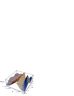
Figure 2:

We stress that a distinctive feature of our scheme is the non-vanishing contribution of the external components of the gauge field to the potential $V_{1}$ in $W$. It is precisely this feature which makes possible to obtain an absolute classically stable compactification after inflation [52] and that is responsible for some of the dependence of the wave function in the number, $d$, of internal dimensions [7]. It is also in this respect that our work contracts with previous one in the literature such as for instance the 6-dimensional Einstein-Maxwell model with an “internal” magnetic monopole discussed in Ref. [55] and the model where gravity is coupled with an “internal” $(D-4)$th rank antisymmetric tensor of Ref. [56]. Our results are although more general, consistent with the ones of the those references in the particular situation where the external components of the gauge field vanish.

We summarize our conclusions as follows. The issue of stability of solutions and the presence of correlations in the quantum case can only be properly addressed via Ansätze for the fields that account for the dynamical degrees of freedom consitently with internal and spacetime symmetries. Moreover, our results demonstrate that once the four-dimensional cosmological constant is constrained to is observational upper bound and the corresponding $D$-dimensional one is chosen in order to allow the stability of the internal dimensions, then the wave function clearly exhibits a correlation between compactification of internal dimensions and expansion of the external ones. This illustrates how a phenomenological requirement help in choosing the ground state of the theory in hand and the way quantum cosmology may be regarded as yet another procedure to select the vacuum of unification theories describing our four-dimensional world.

It is a pleasure to thank Pedro D. Fonseca for a careful reading of the original manuscript and for many relevant suggestions. I would like also to express my gratitude to the organizing committee of the Second Conference on Constrained Dynamics and Quantum Gravity and, in particular, to Vittorio De Alfaro and Marco Cavaglià for the friendship over the years and for the warm hospitality in Santa Margherita.

References

- [1] A. Font, L.E. Ibáñez, D. Lüst and F. Quevedo, Phys. Lett. B245 (1990) 401; B249 (1990) 35.
- [2] E. Alvarez and M. Osorio, Phys. Rev. D40 (1989) 1150.
- [3] A. De La Macorra and S. Lola, Phys. Lett. B373 (1996) 299.
- [4] M.C. Bento and O. Bertolami, Phys. Lett. B384 (1996) 98.
- [5] O. Bertolami, D. Colladay, V.A. Kostelecký and R. Potting, “CPT Violation and Baryogenesis” (hep-ph 9612437); to appear in Phys. Lett. B.
- [6] V.A. Kostelecký and R. Potting, Nucl. Phys. B359 (1991) 545; Phys. Rev. D51 (1995) 3923; Phys. Lett. B381 (1996) 389.
- [7] O. Bertolami, P.D. Fonseca and P.V. Moniz, “Quantum Cosmological Multidimensional Einstein-Yang-Mills Model in a Topology” (gr-qc 9607015).
- [8] M. Dine and N. Seiberg, Phys. Lett. B162 (1986) 299.
- [9] P. Binétruy and M.K. Gaillard, Phys. Rev. D34 (1986) 3069.
- [10] R. Brustein and P.J. Steinhardt, Phys. Lett. B302 (1993) 196.
- [11] G.G. Ross and S. Sarkar, Nucl. Phys. B461 (1996) 597.
- [12] M.C. Bento and O. Bertolami, Phys. Lett. B365 (1996) 59.
- [13] G.D. Coughlan, W. Fischler, E.W. Kolb, S. Raby and G.G. Ross, Phys. Lett. B131 (1983) 59.
- [14] J. Ellis, D.V. Nanopoulos and M. Quirós, Phys. Lett. B174 (1986) 176.
- [15] O. Bertolami, Phys. Lett. B209 (1988) 277.
- [16] B. de Carlos, J.A. Casas, F. Quevedo and E. Roulet, Phys. Lett. B318 (1993) 447.
- [17] M.C. Bento and O. Bertolami, Phys. Lett. B336 (1994) 6.
- [18] T. Banks, D.B. Kaplan and A.E. Nelson, Phys. Rev. D49 (1994) 779.
- [19] T. Banks, M. Berkooz and P.J. Steinhardt, Phys. Rev. D52 (1995) 705.
- [20] M.C. Bento and O. Bertolami, Gen. Rel. and Gravitation 28 (1996) 565.
- [21] T. Banks, M. Berkooz, S.H. Shenker, G. Moore and P.J. Steinhardt, Phys. Rev. D52 (1995) 3548.
- [22] A. Linde, Phys. Lett. B372 (1994) 208.
- [23] A. Vilenkin, Phys. Rev. Lett. 72 (1994) 3137.
- [24] S. Ferrara, D. Lüst, A. Shapere and S. Theisen, Phys. Lett. B225 (1989) 363.
- [25] A.D. Sakharov, JETP Lett. 5 (1967) 24.
- [26] M. Yoshimura, Phys. Rev. Lett. 41 (1978) 281; Phys. Lett. B88 (1979) 294.
- [27] A.Yu. Ignatiev, N.V. Krasnikov, V.A. Kuzmin and A.N. Tavkhelidze, Phys. Lett. B76 (1978) 436.
- [28] S. Dimopoulos and L. Susskind, Phys. Rev. D 18 (1978) 4500.
- [29] S. Weinberg, Phys. Rev. Lett. 42 (1979) 850.
- [30] M. Claudson, L.J. Hall and I. Hinchliffe, Nucl. Phys. B241 (1984) 309.
- [31] K. Yamamoto, Phys. Lett. B168 (1986) 341.
- [32] O. Bertolami and G.G. Ross, Phys. Lett. B183 (1987) 163.
- [33] I. Affleck and M. Dine, Nucl. Phys. B249 (1985) 361.
- [34] V.A. Kuzmin, V.A. Rubakov and M.E. Shaposhnikov, Phys. Lett. B155 (1985) 36.
- [35] V.A. Kuzmin, V.A. Rubakov and M.E. Shaposhnikov, Phys. Lett. B191 (1987) 171.
- [36] A.D. Dolgov and Ya.B. Zeldovich, Rev. Mod. Phys. 53 (1981) 1.
- [37] A.G. Cohen and D.B. Kaplan, Phys. Lett. B199 (1987) 251; Nucl. Phys. B308 (1988) 913.
- [38] D. Colladay and V.A. Kostelecký, Phys. Lett. B344 (1995) 259; Phys. Rev. D52 (1995) 6224; V.A. Kostelecký and R. Van Kooten, Phys. Rev. D54 (1996) 5585.
- [39] J. Ambjorn and A. Krasnitz, Phys. Lett. B362 (1995) 97.
- [40] V.A. Rubakov and M.E. Shaposhnikov, Uspekhi Fiz. Nauk 166 (1996) 493 (hep-ph/9603208).
- [41] M. Yoshimura, Phys. Rev. Lett. 66 (1991) 1559.
- [42] M.C. Bento, O. Bertolami and P.M. Sá, Mod. Phys. Lett. A7 (1992) 911.
- [43] P. Candelas, G.T. Horowitz, A. Strominger and E. Witten, Nucl. Phys. B258 (1985) 46.
- [44] J.B. Hartle and S.W. Hawking, Phys. Rev. D28 (1983) 2960.
- [45] S. Coleman, Nucl. Phys. B307 (1988) 867.
- [46] G. Veneziano, Phys. Lett. B265 (1991) 287.
- [47] A.A. Tseytlin, Mod. Phys. Lett. 6 (1991) 1721.
- [48] M.C. Bento and O. Bertolami, Class. Quantum Gravity 12 (1995) 1919.
- [49] M. Gasperini, J. Maharana and G. Veneziano, Nucl. Phys. B472 (1996) 349.
- [50] A. Lukas and R. Poppe, “Decoherence in Pre-Big-Bang Cosmology” (hep-th/9603167).
- [51] O. Bertolami, J.M. Mourão, R.F. Picken and I.P. Volobujev, Int. J. Mod. Phys. A6 (1991) 4149.
- [52] O. Bertolami, Yu.A. Kubyshin and J.M. Mourão, Phys. Rev. D45 (1992) 3405.
- [53] O. Bertolami and J.M. Mourão, Class. Quantum Gravity 8 (1991) 1271.
- [54] O. Bertolami and P.V. Moniz, Nucl. Phys. B439 (1995) 259.
- [55] J.J. Halliwell, Nucl. Phys. B266 (1986) 228.
- [56] U. Carow-Watamura, T. Inami and S. Watamura, Class. Quantum Gravity 4 (1987) 23.