4D diffeomorphisms in canonical gravity and abelian deformations

Frank Antonsen^∗ and Fotini Markopoulou

Theoretical Physics Group

Blackett Laboratory

Imperial College of Science, Technology and Medicine

London SW7 2BZ

February 21, 1997

Abstract

A careful study of the induced transformations on spatial quantities due to 4-dimensional spacetime diffeomorphisms in the canonical formulation of general relativity is undertaken. Use of a general formalism, which indicates the rôle of the embedding variables in a transparent manner, allows us to analyse the effect of 4-dimensional diffeomorphisms more generally than is possible in the standard ADM approach. This analysis clearly indicates the assumptions which are necessary in order to obtain the ADM–Dirac constraints, and furthermore shows that there are choices, other than the ADM hamiltonian constraint, that one can make for the deformations in the “timelike” direction. In particular an abelian generator closely related to true time evolution appears very naturally in this framework. This generator, its relation to other abelian scalars discovered recently, and the possibilities it provides for a group theoretic quantisation of gravity are discussed.

^∗ Permanent address: Niels Bohr Institute, Blegdamsvej 17, DK 2100 Copenhagen Ø, Denmark
email addresses: antonsen@nbivax.nbi.dk, f.markopoulou@ic.ac.uk

1 Introduction

The standard ADM formulation of canonical general relativity [1, 2] may be considered as an initial value problem, defined by considering initial canonical data on a arbitrary spatial slice in a spacetime foliated by a stack of such slices. The spatial slice, let us call it $\Sigma_{t}$ (assuming that it is a collection of equal-time points), has a 3-metric, $g_{ij}(x)$, inherited from the 4-metric, $\gamma_{\alpha\beta}(X)$ of the surrounding spacetime ${\cal M}$ and a momentum $p^{ij}(x)$ conjugate to the metric. One uses this spatial slice to orient an orthogonal basis $(Nn^{\alpha},N^{i}X^{\mu}_{i})$, defined by the direction normal to the slice, $n^{\mu}$, and the three tangential directions $X^{\mu}_{i}\equiv\frac{\partial X^{\mu}}{\partial x^{i}}$. $N$ and $N^{i}$ are the lapse and shift. Any quantity of interest from covariant general relativity is then decomposed with respect to this basis. Thus, the canonical theory is obtained by decomposing the Hilbert-Einstein action with respect to $(Nn^{\mu},N^{i}X^{\mu}_{i})$. The result describes how the canonical data $g_{ij}(x)$ and $p^{ij}(x)$ are propagated in these four directions by four constraints, the hamiltonian constraint ${\cal H}_{\perp}$ in the normal direction and the momentum constraints ${\cal H}_{i}$ tangentially.

We shall be specifically concerned with the ${\cal H}_{\perp},\ {\cal H}_{i}$ constraints as generators of normal and tangential deformations in the sense described above (as proven in [3]). For the canonical representation of the Einstein theory, one also requires the algebra of the constraints to describe the result of one deformation followed by another. This is usually referred to as the Dirac algebra:

$$\left\{{\cal H}_{\perp}(x),{\cal H}_{\perp}(x^{\prime})\right\} = g^{ij}(x){\cal H}_{i}(x)\delta_{,j}(x,x^{\prime})-(x\leftrightarrow x^{\prime})$$ (1)

$$\left\{{\cal H}_{\perp}(x),{\cal H}_{j}(x^{\prime})\right\} = {\cal H}_{\perp,i}(x)\delta(x,x^{\prime})+{\cal H}_{\perp}(x)\delta_{,i}(x,x^{\prime})$$ (2)

$$\left\{{\cal H}_{i}(x),{\cal H}_{j}(x^{\prime})\right\} = {\cal H}_{j}(x)\delta_{,i}(x,x^{\prime})-(ix\leftrightarrow jx^{\prime}).$$ (3)

The last line in the Dirac algebra, the Poisson bracket between the two momentum constraints, is the statement of ${\rm Diff}\Sigma$ invariance on $\Sigma_{t}$: one spatial deformation followed by another is equivalent to an overall spatial deformation. The second line is simply the transformation of ${\cal H}_{\perp}(x)$ as a scalar of density of weight 1 under ${\rm Diff}\Sigma$. One needs to be more careful with the first line, the Poisson bracket of two hamiltonian constraints. As Hojman, Kuchař and Teitelboim explain in [3], this bracket describes how, if one uses ${\cal H}_{\perp}$ to move from an initial to a final slice via an intermediate one, the arrival point on the final slice depends on the choice of the intermediate slice. This path-dependence of the ${\cal H}_{\perp}$ deformation makes the hamiltonian constraint somewhat difficult to use, and is responsible for the explicit appearance of the metric field $g^{ij}(x)$ in the right hand side of the $\left\{{\cal H}_{\perp}(x),{\cal H}_{\perp}(x^{\prime})\right\}$ Poisson bracket.

This is a very problematic feature of the Dirac algebra. The metric $g^{ij}(x)$ is not a structure constant but one of the fields, which means that the Dirac algebra is not a true Lie algebra. The existence of powerful group theoretic techniques which may be employed in the quantisation of theories classically described by Lie algebras means that the right hand side of this Poisson bracket is unfortunate. It stands as an obstacle to any attempt to apply group theoretic quantisation methods to the dynamical part of the canonical gravity theory.

In this paper we shall reconsider the Dirac algebra, listing which assumptions of the ADM analysis make it unavoidable, and keeping an open mind for alternative algebras of generators of deformations in pure gravity. The motivation for this work was the discovery by Brown and Kuchař of a candidate algebra for gravity of the form Abelian$\times{\rm Diff}\Sigma$ [6]. It was discovered in the context of a non–derivative coupling of incoherent dust to gravity. Performing a canonical decomposition of the system, they found the surprising result that the dust field helped one to select a particular scalar combination of the gravitational constraints, a quantity consisting purely of gravitational variables which, furthermore, had the property of being abelian. More specifically, for incoherent dust, this scalar is $G(x):={\cal H}_{\perp}^{2}(x)-g^{ij}(x){\cal H}_{i}(x){\cal H}_{j}(x)$ (or rather its square root) and satisfies $\{G(x),G(x^{\prime})\}=0$.

Brown and Kuchař concluded with a promising proposal. The scalar density $G$ is a function of the gravitational variables, like the hamiltonian constraint ${\cal H}_{\perp}$, and thus if one used $G$ instead of ${\cal H}_{\perp}$, together with the standard ${\rm Diff}\Sigma$ constraints, the algebra for gravity would not be the problematic Dirac algebra but would instead have the form Abelian$\times{\rm Diff}\Sigma$. At first sight, it is unclear how this proposal can be implemented. For example, $G(x)$ is quadratic in the old constraints and hence, if the dust field is removed, it does not generate motion on the constraint surface of pure gravity. This problem does not arise if the gravitational field remains coupled to some matter field. Consequently, the dilemma arises as to whether the abelian constraints should be investigated in the context of reference fluids and clocks, or in pure gravity. The first option avoids the above problem and has been investigated in [7, 8, 9] who generalised [6] to scalar fields and perfect fluids and discovered even more abelian scalar densities, which we shall term Kuchař constraints. However, this sidesteps the most intriguing feature of these scalars, the fact that they only involve gravity variables.

It has been shown recently [10] that for pure gravity there is a whole family of such abelian scalar densities, including those found via particular matter couplings, which are solutions of a nonlinear partial differential equation. Such a Kuchař scalar density ${\cal K}[({\rm det}g),{\cal H}_{\perp},{\cal H}_{i}]$ of weight $\omega$ can be incorporated in the “Kuchař algebra”

$$\left\{{\cal K}(x),{\cal K}(x^{\prime})\right\} = 0,$$ (4)

$$\left\{{\cal K}(x),{\cal H}_{i}(x^{\prime})\right\} = {\cal K}_{,i}(x)\delta(x,x^{\prime})+\omega{\cal K}(x)\delta_{,i}(x,x^{\prime}),$$ (5)

$$\left\{{\cal H}_{i}(x),{\cal H}_{j}(x^{\prime})\right\} = {\cal H}_{j}(x)\delta_{,i}(x,x^{\prime})-(ix\leftrightarrow jx^{\prime}).$$ (6)

In the present paper, the discovery of the Kuchař scalars and algebra is only the motivation for a search for abelian generators of deformations in pure gravity. We will not attempt here to derive the precise form of the Kuchař scalars from our results, although we discuss a possible relationship. Our focus is evolution as an abelian timelike deformation produced by scalar generators. We shall identify how the hamiltonian constraint and its algebra is tied to the ADM concept of spatial slices and the normal to the slice, which is unrelated to genuine time evolution. We find that, if the 3+1 split does not follow the convenient route of the orthogonal basis of lapse and shift, one can find scalar generators of abelian deformations which have a close relationship to time evolution.

The interesting feature is that the most suitable method for obtaining the above results is to consider the long-standing issue of the rôle of spacetime diffeomorphisms in the canonical theory. We shall discuss how spacetime diffeomorphisms can be handled canonically if one takes into account the ways in which the space $\Sigma$ is embedded in spacetime ${\cal M}$ (for globally hyperbolic spacetime, ${\cal M}\sim\Sigma\times R$) and how ${\rm Diff}{\cal M}$ is hidden in the ADM analysis because this embedding is treated as fixed. A more suitable picture of spacetime ${\cal M}$ as a bundle with fibres $R$ over space $\Sigma$, which naturally accommodates embeddings, is proposed in section 2. In section 3, we use this picture to write down induced spacetime diffeomorphisms on spatial objects. We then move closer to the usual representation of deformations in canonical theory by writing the induced spacetime diffeomorphisms as Lie derivatives on tensor quantities, for example the 3-metric $g_{ij}(x)$ (section 4). From these general transformations, for particular choices of diffeomorphisms and embeddings, one can derive the usual ADM-Dirac generators and understand more precisely the assumptions that go into the construction of the normal deformation by the hamiltonian constraint, as we show in section 5. Interestingly, we also find a generator which is in many ways more natural than the hamiltonian constraint corresponding to diffeomorphisms along the $R$ fibre. This constraint is abelian and, in contrast to the hamiltonian constraint, the evolution it generates can be more naturally associated with timelike evolution. This particular choice is discussed in Section 6, and the consequences for quantisation, along with other concluding remarks are given in Section 7.

2 ${\rm Diff}{\cal M}$ and the embedding of $\Sigma$ in ${\cal M}$

The 4-dimensional formulation of general relativity is covariant under diffeomorphisms (${\rm Diff}{\cal M}$) of the spacetime manifold ${\cal M}$. In order to develop a Hamiltonian formulation for the purposes of canonical quantisation one must introduce a 3+1 split of spacetime into space and time. While not manifestly covariant, it is clear that this representation must still exhibit the symmetries of the 4-dimensional theory if only in terms of an arbitrariness of the embedding of the spatial slice. The actual question of how the ${\rm Diff}{\cal M}$ covariance is realised in the canonical theory is clearly of importance. However, the ADM formulation is not necessarily the most appropriate formalism in which to address this question. While in 4 dimensions we have the ${\rm LDiff}{\cal M}$ algebra, in the ADM formalism the only algebraic-like structure is the Dirac algebra. It is accepted that the Dirac algebra is, somehow, the “projection” of ${\rm LDiff}{\cal M}$ onto the foliated spacetime. However, this is not a clear statement. The Dirac algebra is very far from being either isomorphic or a subalgebra of ${\rm LDiff}{\cal M}$ since it is not even a true algebra.

Recovering ${\rm Diff}{\cal M}$ in the canonical theory is difficult, essentially because a fundamental tenet of a canonical theory is not to have explicit reference to what appears as ambient spacetime. Fortunately, as has been pointed out in detail by Isham and Kuchař [15], there is indeed a link provided between space and spacetime. It is encoded in the way space is thought of as embedded in spacetime in a 3+1 theory. That is, in the common assumption of a globally hyperbolic spacetime, ${\cal M}\sim\Sigma\times R$, there are many ways in which $\Sigma$ is embedded in ${\cal M}$ (provided the metric induced on $\Sigma$ can be spacelike). However, in the ADM approach once the 3+1 decomposition is accomplished one appears to lose contact with details of the embedding.

In order to carefully analyse the realisation of 4-dimensional symmetries in the 3+1 theory it is clearly necessary to have explicit reference to the embedding information at the canonical level. For this reason it is important to know at which stage of the ADM approach one loses the explicit embedding information, at least in the sense to which this information is arbitrary and one can modify the particular embedding if required.

The procedure of the decomposition is to assume that ${\cal M}$ is foliated by (equal-time) spacelike slices $\Sigma_{t}$. If we label coordinates in ${\cal M}$ by $X^{\alpha}$ and in $\Sigma_{t}$ by $x^{i}$, then the Jacobian $X^{\mu}_{i}:={\partial X^{\mu}\over\partial x^{i}}$ describes the way that $\Sigma_{t}$ is embedded in ${\cal M}$. Each slice $\Sigma_{t}$ acquires a 3-metric which is the projection of the spacetime metric $\gamma_{\alpha\beta}$ on an orthogonal basis defined on the slice via the decomposition of the deformation vector $\dot{X}^{\mu}$ (where the dot denotes differentiation by time):

$$\dot{X}^{\mu}=Nn^{\mu}+N^{i}X^{\mu}_{i}.$$ (7)

However, to use this formula in the canonical analysis one needs to treat the embedding $X^{\mu}_{i}$ as fixed. For fixed $X^{\mu}_{i}$ the spacetime ${\cal M}$ becomes a particular stack of slices $\Sigma_{t}$ for increasing $t$. This construction is of course general since (7) holds for all $X^{\mu}_{i}$ (producing spacelike slices). However if, at the level of the canonical theory, one wishes to see what happens when the embedding changes one needs to return to (7) and perform the analysis more generally. Note that otherwise the choice of decomposition has an effect similar to the partial “gauge-fixing” of a theory where certain invariances of the theory, while still present in the sense that the choice of “gauge” is arbitrary, become hidden. In this context we no longer have ${\cal M}\sim\Sigma\times R$ for all possible embeddings $\Sigma\rightarrow{\cal M}$, but only for a chosen, albeit arbitrary, example. As a result, this fixing of the embedding hides the ${\rm Diff}{\cal M}$ covariance of the theory.

The ADM construction is based on this assumption of fixing the embedding and some of its features are natural only in this context. Among the basic objects associated with eq. (7) are the geometric spatial slice and its normal direction, which naturally lead to the hamiltonian constraint being the generator of normal deformations. In a formulation where the embeddings can be modified, the spatial slice and its normal will be less fundamental features.

As the preceding discussion has indicated, in order to describe spacetime diffeomorphisms we require a canonical split that can accommodate arbitrary embeddings. We shall now outline a straightforward formalism of this type which relies on the use of the global hyperbolicity requirement ${\cal M}\sim\Sigma\times R$.

Figure 1: Spacetime ${\cal M}$ as a bundle over space $\Sigma$.

We consider a 3-dimensional manifold $\Sigma$, whose metric is not yet specified. Over each point $x$ of $\Sigma$, there is an $R$-line. This results in a line bundle ${\cal M}$ over $\Sigma$ with fibre $R$:

$$\begin{array}[]{ccc}R&\longrightarrow&{\cal M}\\ &&\pi\downarrow\uparrow\sigma\\ &&\Sigma\end{array}$$ (8)

as pictured in figure 1. There is a projection map, $\pi:{\cal M}\rightarrow\Sigma$, and the cross-section map $\pi\circ\sigma=1$. The actual embedding then corresponds to this cross-section map $\sigma$, as it takes each point $x\in\Sigma$ to a point $\sigma(x)$ in ${\cal M}$. Thus, for every $\sigma$ we have an embedding of the 3-dimensional manifold $\Sigma$ in ${\cal M}$, which we will denote by $\sigma(\Sigma)$. This cross-section $\sigma(\Sigma)$ is the spatial slice in the ADM language.

The bundle ${\cal M}$ is ${\rm Diff}{\cal M}$ covariant. Under a diffeomorphism $\phi\in{\rm Diff}{\cal M}$, $\sigma(x)\in{\cal M}$ is mapped to $\phi^{-1}\sigma(x)\in{\cal M}$. The maps $\sigma$, and $\pi$ connect $\Sigma$ and ${\cal M}$ in a natural way. For example, when in ${\cal M}$, we can act with $\phi\in{\rm Diff}{\cal M}$, and finally return to $\pi\phi^{-1}\sigma(x)\in\Sigma$ using the projection map $\pi$. As a consequence this bundle construction allows us to induce spacetime transformations on spatial objects. The induced spatial transformation is from $x$ to $\pi\phi^{-1}\sigma(x)\in\Sigma$.

In the next two sections, we shall work out explicitly the induced ${\rm Diff}{\cal M}$ transformations of spatial objects.

3 Induced spacetime diffeomorphisms on space

Let us first consider the simplest case, the transformation induced by a diffeomorphism $\phi\in{\rm Diff}{\cal M}$ on a vector $v_{x}\in T_{x}\Sigma$. According to figure 1, we can push this vector forward through

$$T_{x}\Sigma\stackrel{{\scriptstyle\sigma_{*}}}{{\longrightarrow}}T_{\sigma(x)}{\cal M}\stackrel{{\scriptstyle\phi_{*}}}{{\longrightarrow}}T_{\phi^{-1}\sigma(x)}{\cal M}\stackrel{{\scriptstyle\pi_{*}}}{{\longrightarrow}}T_{\pi\phi^{-1}\sigma(x)}\Sigma$$ (9)

sending

$$v_{x}\in T_{x}\Sigma\mapsto\sigma_{*}v_{x}\mapsto\phi_{*}\sigma_{*}v_{x}\mapsto\pi_{*}\phi_{*}\sigma_{*}v_{x}\in T_{\pi\phi^{-1}\sigma(x)}\Sigma.$$ (10)

In order to evaluate the result we begin with a basis $\left({\partial/\partial x^{i}}\right)_{x}$ in $T_{x}\Sigma$ with respect to which $v_{x}$ has components

$$v_{x}=v^{i}\left({\partial\over\partial x^{i}}\right)_{x}.$$ (11)

Then if $\left(\partial/\partial X^{\mu}\right)_{\sigma(x)}$ is a basis in $T_{\sigma(x)}{\cal M}$ we can use the Jacobian for the two bases,

$$\sigma^{\mu}_{,i}(x):=\left(\frac{\partial X^{\mu}(x)}{\partial x^{i}}\right)_{\sigma(x)},$$ (12)

to obtain the push-forward $\sigma_{*}v_{x}$ of $v_{x}$ as

$$\sigma_{*}v_{x}\in T_{\sigma(x)}{\cal M}=v^{i}\sigma^{\mu}_{,i}(x)\left({\partial\over\partial X^{\mu}}\right)_{\sigma(x)}.$$ (13)

We now have a vector $\sigma_{*}v_{x}$ in $T_{\sigma(x)}{\cal M}$ on which we can apply a 4-dimensional diffeomorphism $\phi\in{\rm Diff}{\cal M}$ and obtain

$$\phi_{*}\sigma_{*}v_{x}\in T_{\phi^{-1}\sigma(x)}{\cal M}=v^{i}\sigma^{\mu}_{,i}(x)\phi^{\nu}_{,\mu}\left(\sigma(x)\right)\left({\partial\over\partial X^{\nu}}\right)_{\phi^{-1}\sigma(x)}.$$ (14)

Finally, we can push this forward to $T\Sigma$ again, using the Jacobian $\pi^{j}_{,\nu}\left(\phi^{-1}\sigma(x)\right)$ for the two bases $\left({\partial\over\partial X^{\nu}}\right)_{\phi^{-1}\sigma(x)}$ and $\left({\partial\over\partial x^{j}}\right)_{\pi\phi^{-1}\sigma(x)}$,

$$\pi^{j}_{,\nu}\left(\phi^{-1}\sigma(x)\right)=\left(\frac{\partial x^{j}(X^{\nu})}{\partial X^{\nu}}\right)_{\phi^{-1}\sigma(x)},$$ (15)

to obtain

$$\pi_{*}\phi_{*}\sigma_{*}v_{x}=v^{i}\sigma^{\mu}_{,i}(x)\phi^{\nu}_{,\mu}\left(\sigma(x)\right)\pi^{j}_{,\nu}\left(\phi^{-1}\sigma(x)\right)\left({\partial\over\partial x^{j}}\right)_{\pi\phi^{-1}\sigma(x)}.$$ (16)

Combining the results above, the induced spacetime diffeomorphism on the spatial vector $v_{x}$ has the component form

$$v^{i}_{x}\mapsto v^{\prime j}_{\pi\phi^{-1}\sigma(x)}=v^{i}\sigma^{\mu}_{,i}(x)\phi^{\nu}_{,\mu}\left(\sigma(x)\right)\pi^{j}_{,\nu}\left(\phi^{-1}\sigma(x)\right).$$ (17)

This equation may be readily extended to a spatial vector field. This is because, when $x$ is varied smoothly and continuously over all $\Sigma$ in (17), this transformation remains well-defined. It can therefore be used to push-forward vector fields.

Let us now turn to 1-forms and covectors. In this case it is easier to write down the induced ${\rm Diff}{\cal M}$ pullback if we reverse the route used in the analysis of vectors. In other respects the derivation is very similar to that above. The component result of the pullback of the one-form $\omega(\pi\phi^{-1}\sigma(x))$ to $\omega^{\prime}(x)$ via $\sigma^{*}\phi^{*}\pi^{*}$ is

$$\omega^{\prime}_{j}(x)\in T_{x}^{*}\Sigma=\omega_{j}\left(\pi\phi^{-1}\sigma(x)\right)\pi^{j}_{,\nu}\left(\phi^{-1}\sigma(x)\right)\phi^{\nu}_{,\mu}\left(\sigma(x)\right)\sigma^{\mu}_{,i}(x)\left(dx^{i}\right)_{x}.$$ (18)

Similarly, the covector transformation $k^{\prime}\in T^{*}_{\pi\phi^{-1}\sigma(x)}\Sigma\rightarrow k\in T^{*}_{x}\Sigma$ is

$$k_{j}(x)=k^{\prime}_{j}\pi^{j}_{,\nu}\left(\phi\sigma(x)\right)\phi^{\nu}_{\mu}\left(\sigma(x)\right)\sigma^{\mu}_{i}(x)\left(dx^{i}\right)_{x}.$$ (19)

One can check that $k$ and $v$, as given by the formulae above, are indeed dual i.e. $\langle k,\pi_{*}\phi_{*}\sigma_{*}v\rangle_{\pi\phi^{-1}\sigma(x)}=\langle\sigma^{*}\phi^{*}\pi^{*}k,v\rangle_{x}$.

4 Infinitesimal spacetime diffeomorphisms on spatial tensors

At this stage, we have coordinate expressions for the transformations of the simplest tensorial objects and it is straightforward to extend these results to other spatial objects as required. Let us now return to our initial problem, the relation between ${\rm Diff}{\cal M}$ and the deformations generated by constraints. We would like to compare the present formalism to the standard approach of constraint generators decomposed with respect to a fixed orthogonal basis. For example, we can consider the tangential deformation of the 3-metric by the momentum constraint ${\cal H}_{i}$ (smeared by a vector field $N$):

$$\left\{{\cal H}(N),g_{ij}\right\}=\delta g_{ij}={\cal L}_{N}g_{ij}.$$ (20)

We need to work with infinitesimal $\phi\in{\rm Diff}{\cal M}$, namely, Lie derivatives with respect to a vector field ${\cal V}\in T{\cal M}$. Such an infinitesimal diffeomorphism transforms, say, the covector $\xi\in T^{*}{\cal M}$ in the manner

$$\xi\mapsto\xi^{\prime}=\xi+\epsilon{\cal L}_{\cal V}\xi+{\cal O}\left(\epsilon^{2}\right).$$ (21)

Recall that the base space $\Sigma$ does not have a fixed 3-metric $g_{ij}(x)$, unlike a spatial slice $\Sigma_{t}$. Instead, for $\Sigma$, $g_{ij}(x)$ is a special symmetric 2-index tensor, an element of $T^{*}_{x}\Sigma\otimes T^{*}_{x}\Sigma$. Its deformation (20) will then be a particular induced ${\rm Diff}{\cal M}$ map $\sigma_{*}\phi_{*}\pi_{*}:T^{*}_{x}\Sigma\otimes T^{*}_{x}\Sigma\rightarrow T^{*}_{\pi\phi^{-1}\sigma(x)}\Sigma\otimes T^{*}_{\pi\phi^{-1}\sigma(x)}\Sigma$, as we shall verify in section 5.

In preparation let us write down the induced spacetime diffeomorphism of a general tensor in $T^{*}_{x}\Sigma\otimes T^{*}_{x}\Sigma$, say $t_{ij}(x)$. The result follows in a similar manner to the calculations already presented, except that transformations are required for each index and we consider only infinitesimal diffeomorphisms with parameter $\epsilon$, i.e.

$$t^{\prime}_{ij}=t_{ij}+\epsilon\sigma^{\mu}_{,i}\sigma^{\nu}_{,j}\left[{\cal V}^{\lambda}t_{\mu\nu}+\left(\partial_{\mu}{\cal V}^{\lambda}\right)t_{\lambda\nu}+\left(\partial_{\nu}{\cal V}^{\lambda}\right)t_{\lambda\mu}\right],$$ (22)

where $t_{\mu\nu}$ (at $\sigma(x)$) is shorthand for $t_{ij}(x)$ embedded in ${\cal M}$:

$$t_{ij}(x)=\sigma^{\mu}_{,i}(x)\sigma^{\nu}_{,j}(x)t_{\mu\nu}\left(\sigma(x)\right).$$ (23)

Similarly, for a contravariant 2-tensor, $l^{ij}\in T\Sigma\otimes T\Sigma$, we have

$$l^{\prime ij}=l^{ij}+\epsilon\pi^{i}_{,\mu}\pi^{j}_{,\nu}\left[{\cal V}^{\lambda}l^{\mu\nu}+\left(\partial_{\mu}{\cal V}^{\lambda}\right)l^{\lambda\nu}+\left(\partial_{\nu}{\cal V}^{\lambda}\right)l^{\lambda\mu}\right].$$ (24)

The transformations (22) and (24) are general formulae that encode the induced action of arbitrary 4-dimensional infinitesimal diffeomorphisms on spatial 2-tensors. The compactness of these expressions hides the fact that most of the physical information is contained in the sets of $\sigma^{\mu}_{,i}$ and the choice of the vector field ${\cal V}^{\mu}$. Recall that $\sigma^{\mu}_{,i}$ are the coordinate expressions for the embedding $T\Sigma\rightarrow T{\cal M}$ induced by the cross-sections $\sigma:\Sigma\rightarrow{\cal M}$. The choice of the vector field ${\cal V}^{\mu}$ is determined by the spacetime diffeomorphism $\phi\in{\rm Diff}{\cal M}$ we are performing.

In the next two sections we show that, as special cases of (22) and (24), we can, firstly retrieve the Dirac algebra explicitly as an orthogonal projection of spacetime diffeomorphisms on $\Sigma\times R$ and, secondly, obtain abelian transformations generated by an extra class of diffeomorphisms along the $R$-fibre. These arise very naturally, are by construction abelian, and suggest intriguing connections to existing 3+1 work.

5 The ADM-Dirac generators as projections of ${\rm LDiff}{\cal M}$ on an orthogonal basis

Having developed a formalism for considering the transformation of spatial tensors under 4-dimensional diffeomorphisms of the bundle ${\cal M}$ that explicitly involves “embeddings”, we may use it for the Dirac algebra of the canonical constraints. Appropriate conditions on the vector field ${\cal V}$ via which the Lie derivatives of the transformations (22) and (24) are defined and the embedding $\sigma$ will reproduce the hamiltonian and momentum constraints as generators of spatial and normal diffeomorphisms.

We begin by using (22) to derive the known deformations of the 3-metric $g_{ij}(x)$ under the momentum and hamiltonian constraints [11]. Recall that for the purpose of considering the effect of spacetime diffeomorphisms $g_{ij}(x)$ may be regarded as a tensor of the form $t_{ij}(x)\in T^{*}\Sigma\otimes T^{*}\Sigma$. That is, its transformation under a general infinitesimal spacetime diffeomorphism is given by equation (22),

$$g^{\prime}_{ij}=g_{ij}+\epsilon\sigma^{\mu}_{,i}\sigma^{\nu}_{,j}\left[{\cal V}^{\lambda}g_{\mu\nu}+\left(\partial_{\mu}{\cal V}^{\lambda}\right)g_{\lambda\nu}+\left(\partial_{\nu}{\cal V}^{\lambda}\right)g_{\lambda\mu}\right],$$ (25)

with $g_{\mu\nu}(\sigma(x))$ given by $g_{ij}(x)=\sigma^{\mu}_{,i}(x)\sigma^{\nu}_{,j}(x)g_{\mu\nu}(\sigma(x))$. The constraints are then generators of canonical transformations between elements of $T^{*}\Sigma\otimes T^{*}\Sigma$.

A spatial diffeomorphism is generated by a vector field $N$ which is purely spatial, $N\in T\Sigma$. When $\Sigma$ is embedded in ${\cal M}$, the corresponding spacetime diffeomorphism will be with respect to a vector field ${\cal V}$ which lies in the cross-section $\sigma(\Sigma)$, i.e. ${\cal V}^{\mu}(\sigma(x))=\sigma^{\mu}_{,i}(x)N^{i}(x)$. Using the identity $\pi\circ\sigma=1$, namely,

$$\pi^{i}_{,\nu}\left(\sigma(x)\right)\sigma^{\nu}_{,j}(x)=\delta^{i}_{j}(x),$$ (26)

we obtain

$$\pi^{i}_{,\mu}\left(\partial_{k}\sigma^{\mu}_{,j}\right)=-\sigma^{\mu}_{,j}\left(\partial_{k}\pi^{i}_{,\mu}\right),$$ (27)

which, together with the integrability condition

$$\partial_{j}\sigma^{\mu}_{,i}=\partial_{i}\sigma^{\mu}_{,j}$$ (28)

leads to equation (25) reducing to the expected form:

$$g^{\prime}_{ij}(\pi\phi^{-1}\sigma(x))=g_{ij}(x)+\epsilon{\cal L}_{N}g_{ij}(x)$$ (29)

as in equation (20). Therefore, this induced diffeomorphism $g_{ij}\rightarrow g^{\prime}_{ij}$ is indeed an element of ${\rm Diff}\Sigma$.

Let us now check whether, for $\phi$ a diffeomorphism with respect to a vector field normal to the cross-section $\sigma(\Sigma)$, equation (25) reduces to the known normal deformation of the 3-metric generated by the hamiltonian constraint [12],

$$g^{\prime}_{ij}=g_{ij}+\epsilon\left[\partial_{0}g_{ij}+D_{(i}N_{j)}\right],$$ (30)

where $D_{i}$ denotes the spatial covariant derivative. The following derivation is interesting mainly because it shows which are the assumptions of ADM needed to make the hamiltonian constraint and normal deformations a convenient tool to use. Note that in our picture of 3-space arbitrarily embedded in spacetime, the normal is no longer the most natural direction to use in order to describe deformations which are not tangential to the embedded slice, as we shall come to in Section 6.

It turns out that there are four assumptions used in the ADM formulation in order to turn an arbitrary normal deformation, i.e. equation (25) for ${\cal V}^{\mu}$ some normal vector field $n^{\mu}$:

$$g^{\prime}_{ij}=g_{ij}+\epsilon\sigma^{\mu}_{i}\sigma^{\nu}_{j}\left[n^{\lambda}g_{\mu\nu}+\left(\partial_{\mu}n^{\lambda}\right)g_{\lambda\nu}+\left(\partial_{\nu}n^{\lambda}\right)g_{\lambda\mu}\right],$$ (31)

into the simplified form of (30). Firstly, one needs to choose (and fix) the embedding $\sigma$. Once the embedding is fixed, as a second step, the lapse and shift can be introduced, in a manner formally equivalent to the usual decomposition of the deformation vector

$$\dot{X}^{\mu}=n^{\mu}N+X^{\mu}_{i}N^{i}.$$ (32)

In our notation $X^{\mu}_{i}=\frac{\partial X^{\mu}}{\partial x^{i}}\equiv\sigma^{\mu}_{,i}(x)$ and $X^{\mu}\equiv\sigma^{\mu}(x)$, so the lapse and shift will appear through $\partial_{0}\sigma^{\mu}$. Explicitly, and similarly to the case of spatial diffeomorphisms, we can impose integrability to find that

$$\partial_{i}\left(\partial_{0}\sigma^{\mu}\right)=\partial_{0}\sigma^{\mu}_{,i},$$ (33)

which may be decomposed in the same basis as (32) to give

$$\partial_{0}\sigma^{\mu}_{i}=\partial_{i}\left(n^{\mu}N+\sigma^{\mu}_{,i}N^{i}\right).$$ (34)

The general normal diffeomorphism (31) can be simplified to

$$g^{\prime}_{ij}=g_{ij}+\epsilon n^{\lambda}\partial_{\lambda}g_{ab}+\epsilon n^{\lambda}\sigma^{\mu}_{,i}\sigma^{\nu}_{,j}\left[\partial_{\lambda}\left(\pi^{a}_{,\mu}\pi^{b}_{\nu}\right)-\partial_{\mu}\left(\pi^{a}_{,\lambda}\pi^{b}_{,\nu}\right)-\partial_{\nu}\left(\pi^{a}_{,\lambda}\pi^{b}_{,\mu}\right)\right]g_{ab}.$$ (35)

Using the integrability condition (33), and the decomposition (34) we find, after some tedious calculations,

$$g^{\prime}_{ij} = g_{ij}+\epsilon n^{k}\left\{\partial_{k}g_{ij}-\left(\sigma^{\nu}_{,j}\delta^{a}_{[k}\partial_{i]}\pi^{b}_{,\nu}+\sigma^{\mu}_{i}\delta_{[k}\partial_{j]}\pi^{a}_{\mu}\right)g_{ab}\right\}-$$ (36)

$$\epsilon n^{0}\left\{D_{(i}N_{j)}+\partial_{0}g_{ij}-N^{k}\left[\sigma^{\mu}_{,j}\partial_{k}\left(\pi^{a}_{,\mu}g_{ia}\right)+\sigma^{\mu}_{,i}\partial_{k}\left(\pi^{a}_{,\mu}g_{aj}\right)\right]\right\}-$$

$$\left[\delta^{a}_{i}\pi^{b}_{,\mu}\partial_{j}(Nn^{\mu})+\delta^{b}_{j}\pi^{a}_{,\mu}\partial_{i}(Nn^{\mu})\right]g_{ab}+$$

$$\left(\partial_{(i}\sigma^{\mu}_{j)}\right)g_{0\mu}-g_{b(i}\partial_{j)}\pi^{b}_{0}.$$

Requiring that the above transformation $g_{ij}\rightarrow g^{\prime}_{ij}$ be produced by a generator ${\cal F}(g_{ij},p^{ij})$ via $\delta g_{ij}=\{g_{ij},{\cal F}(N)\}$ (by analogy to the usual normal transformation (30) also being the result of the Poisson bracket of the metric with the smeared hamiltonian constraint $\{g_{ij},{\cal H}_{\perp}(N)\}$) we can find ${\cal F}$:

$${\cal F}\left(g_{ij},p^{i},\sigma^{\mu}_{,i}\right)=n^{0}{\cal H}_{\perp}+p^{ij}n^{k}\partial_{k}g_{ij}+p^{ij}A^{ab}_{i}g_{ab}+f(g,\sigma),$$ (37)

where ${\cal H}_{\perp}$ denotes the standard normal deformation as in eq. (30), $p^{ij}$ has been defined to be the time derivative of $g_{ij}$, and the other terms are simply the rest of (36) expressed in a convenient notation. $A^{ab}_{ij}$ is the function of lapse, shift and embedding

$$A^{ab}_{ij} = -n^{k}\left[\sigma^{\nu}_{,j}\delta^{a}_{[k}\partial_{i]}\pi^{b}_{,\nu}+\sigma^{\mu}_{i}\delta^{b}_{[k}\partial_{j]}\pi^{a}_{,\mu}\right]+$$ (38)

$$n^{0}\left[\delta^{a}_{(i}\partial_{j)}\pi^{b}_{,0}-\pi^{a}_{,0}\pi^{b}_{,\mu}\partial_{i}\sigma^{\mu}_{,j}+\pi^{a}_{,\mu}\pi^{b}_{,0}\partial_{j}\sigma^{\mu}_{,i}+\right.$$

$$\left.N^{k}\sigma^{\mu}_{,(i}\partial_{|k}\pi^{a}_{,\mu|}\delta^{b}_{i)}-\delta^{a}_{i}\pi^{b}_{,\mu}\partial_{j}(Nn^{\mu})-\delta^{b}_{j}\pi^{a}_{,\mu}\partial_{i}(Nn^{\mu})\right],$$

and $f(g,\sigma)$ is an unspecified function of the 3-metric and the embedding only.

The generator ${\cal F}$ in (37) is still cumbersome because we are only halfway through imposing the ADM assumptions. As the third step we now “lock” the coordinate frame to our embedding choice, so that $n^{\mu}$ becomes $n^{0}=-1,\ n^{k}=0$. The second term in (37) and the first term in (38) then vanish. Finally, let us assume that the cross-sections are slices of constant coordinate time which implies that $\sigma^{\mu}_{,i}=const$. The last two terms of (37) then vanish as they contain derivatives of $\sigma^{\mu}_{,i}$ and we have recovered the ADM hamiltonian constraint ${\cal H}_{\perp}$.

6 Abelian diffeomorphisms along the $R$-fibre

The derivation in the previous section clarifies the statement that the Dirac algebra is the “projection” of ${\rm LDiff}{\cal M}$. However, this projection is with respect to a basis determined by a spatial slice and its normal direction, rather than on $\Sigma\times R$. In fact, the projection on $\Sigma\times R$, which we are now going to consider, remarkably leads to a generator algebra of the form Abelian$\times{\rm Diff}\Sigma$.

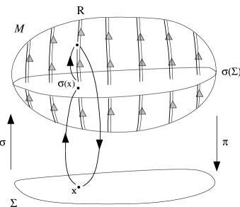
Figure 2: Abelian deformations.

As much as the normal diffeomorphisms were unnatural and rather tedious to recover, this third special class of diffeomorphisms is simple and straightforward to find. It is the case where the spacetime diffeomorphism is a base-point preserving map in the bundle. That is, the vector field ${\cal V}^{\mu}$ is along the 1-dimensional $R$-fibre, as shown in figure 2. By construction, this ${\cal V}^{\mu}$ may be represented as ${\cal V}=\frac{\partial}{\partial\tau}$, $\tau$ being the affine parameter along the fibre. In this case, the transformation (25) of the 3-metric reduces to

$$g^{\prime}_{ij}=g_{ij}+\epsilon\frac{\partial}{\partial\tau}g_{ij}-\epsilon\left(g_{kl}\pi^{k}_{,\mu}\pi^{l}_{,\nu}\right)\frac{\partial}{\partial\tau}\left(\sigma^{\mu}_{,i}\sigma^{\nu}_{,j}\right).$$ (39)

This describes the change in the value of $g_{ij}(x)$ at each point $x\in\Sigma$ after some “time evolution” $\tau$. Note that the first two terms of (39) reflect this time-evolution property of the base-point preserving diffeomorphisms in a straightforward way. The third term depends only on the embedding, which changes in $\tau$-time since it is not restricted to being static in this formalism. Furthermore, because of the simplicity of the spacetime we are dealing with, it is not unexpected that this transformation along the 1-dimensional fibre is abelian. More accurately, our natural assumption that the fibre is an $R$-group acting freely on ${\cal M}$ lets us treat ${\cal M}$ as a principal $R$-bundle. Then the above transformations from ${\cal M}$ to itself form a group, the automorphism group of ${\cal M}$, Aut$({\cal M})$. Moreover, since ${\cal M}$ is trivial, Aut$({\cal M})$ is isomorphic to the group $C^{\infty}(\Sigma,R)$ of functions on $\Sigma$, which is abelian. Thus we have obtained a framework in which the evolution of the embedded slices is naturally described by abelian constraints.

The result is that this projection of ${\rm Diff}{\cal M}$ on $\Sigma\times R$ leads to the Lie algebra $L{{\rm Diff}\Sigma}\odot{C^{\infty}(\Sigma)}$ (with the symbol $\odot$ denoting the semidirect product). One may choose to use the transformation (39) in place of the normal (30) combined with the spatial diffeomorphisms (29) for a 3+1 decomposition with a true Lie algebra of its deformation generators.

The ADM-Dirac algebra and this ${{\rm Diff}\Sigma}\odot{C^{\infty}(\Sigma)}$ algebra are very special cases of the general spacetime deformations (22) and (24) in that they only refer to the 3-space. The ADM-Dirac algebra is constructed from the beginning in this way, starting from a spatial slice and using quantities that can be defined intrinsically to the slice. The ${{\rm Diff}\Sigma}\odot{C^{\infty}(\Sigma)}$ algebra also turns out to have this property as both ${\rm Diff}\Sigma$ and more importantly $C^{\infty}(\Sigma)$ require only $\Sigma$ and not ${\cal M}$ for their definition. In fact, it is possible to derive the results of this paper without reference to spacetime ${\cal M}$ as a physical manifold with 4-metric $\gamma_{\alpha\beta}$, but by starting from a 3-dimensional space $\Sigma$ on which ${\rm Diff}\Sigma$ and $C^{\infty}(\Sigma)$ can be defined. In that context, the 4-dimensional bundle is only a helpful way to unfold transformations under these two groups by raising an $R$-fibre over each spatial point and constructing a $\Sigma\times R$ bundle over $\Sigma$. This approach was followed in [13]. One should note that information about spacetime and the spacetime metric is not used until the very last stages of the derivation of the hamiltonian generator, when “locking” the coordinate frame to the chosen foliation.

7 Conclusions

Motivated by the recent discovery of abelian constraints, and the proposal that these abelian generators could be of use in group theoretic approaches to canonical quantisation [6], we re–analysed the ADM-Dirac algebra and the hamiltonian constraint. We traced the problem of its non-closing Poisson bracket to the selection of a spatial slice and its normal as primary elements of the ADM canonical analysis and the fixed choice of embeddings needed for their use. Allowing variation of the embeddings, which is in principle allowed in the canonical gravity, makes it possible to describe the effect of 4-dimensional spacetime diffeomorphisms, at least when spacetime is globally hyperbolic. In order to include the embeddings, we found it necessary to change our viewpoint of spacetime from a fixed stack-of-slices to spacetime as an ${\cal M}\sim\Sigma\times R$ bundle over a generic 3-manifold $\Sigma$, where the embeddings correspond to the cross-section maps from $\Sigma$ to ${\cal M}$. By including embeddings explicitly in this manner we were able to break ${\rm Diff}{\cal M}$ covariance in a controlled manner in order to obtain the induced ${\rm Diff}{\cal M}$ action on spatial quantities.

Using these general transformations, we were able to perform 3+1 splits of ${\rm Diff}{\cal M}$ corresponding to two different embeddings. A standard normal and tangential split with respect to the spatial slice which leads to the ADM-Dirac algebra, and one on $\Sigma\times R$, leading to an Abelian$\times{\rm Diff}\Sigma$ algebra. The first case was useful in clarifying the ADM assumptions used in the construction of the hamiltonian constraint and showing how they are incompatible with truly variable embeddings. The second split makes use of the $R$ in $\Sigma\times R$, and perhaps not surprisingly, produces abelian deformations whose form resembles time evolution (although we have left open the issue of the rôle of the $R$-fibres). It is important to note that this $L{{\rm Diff}\Sigma}\odot{C^{\infty}(\Sigma)}$ algebra only refers to the space $\Sigma$. Corresponding to the way in which the ADM analysis can be thought of as a foliation of spacetime ${\cal M}$ by spatial slices, the decomposition in terms of the bundle is a fibering of ${\cal M}$ by $R$.

While the existence of an abelian algebra for canonical general relativity is very promising, particularly in the context of group quantisation, there are a number of tasks which need to be performed before deciding whether the Abelian$\times{\rm Diff}\Sigma$ split is of practical use. So far, we have used Lie derivatives to describe infinitesimal transormations. In the sense described in [3] this amounts to constructing the kinematics of the Abelian$\times{\rm Diff}\Sigma$ formulation. The dynamics would describe the change of functionals of the canonical variables $g_{ij}(x)$ and $p^{ij}(x)$ under these transformations using Poisson bracket relationships. This requires finding expressions for our abelian generators in terms of the canonical variables. To find them, one may use the same postulate as [3] and ask that they should “represent the kinematical generators”, that is, they should be constructed from the canonical variables—and the embedding variables in our case—in such a way that their Poisson brackets close like the commutators of the corresponding kinematical generators. We expect the inclusion of the embedding variables to produce interesting results [14] and possible relationship to [15] and [16].

Finally, let us recall the Kuchař scalars. In their derivation in [6, 7, 8] a reference fluid is required to select the particular form of the scalar, and according to [9], each member of the family found in [10] also corresponds to a particular choice of reference fluid. The unsatisfactory element there is that, thus far, each case may only be obtained in a somewhat ad hoc manner. It appears possible to set up an equivalence between the $\sigma$ variables and reference fluids [17], thus providing a better organised derivation of Kuchař scalars and a connection of the present work to the reference fluid results.

References

- [1] Arnowitt R, Deser S and Misner S W 1962 in Gravitation: An Introduction to Current Research, ed Witten L (New York: Wiley)
- [2] Dirac P A M 1964 Lectures on Quantum Mechanics (New York: Yeshiva University)
- [3] Hojman A S, Kuchar K V and Teitelboim C (1971) Ann. Phys. 96 88; Teitelboim C 1979 in General Relativity and Gravitation, ed Held A (New York: Plenum)
- [4] Isham C J 1984 in Relativity, Groups and Topology II, ed DeWitt B S and Stora R (Amsterdam: North-Holland)
- [5] Isham C J and Kakas A C (1984) Class. Quantum Grav. 1 621; 633
- [6] Brown J D and Kuchař K V 1995 Phys. Rev. D 51 5600
- [7] Kuchař K V and Romano J D 1995 Phys. Rev. D 51 5579
- [8] Brown J D and Marolf D 1995 Phys. Rev. D 53 1935
- [9] Kouletsis I 1996 “Action functionals of single scalar fields and arbitrary–weight gravitational constraints that generate a genuine Lie algebra” (gr-qc/9601043) accepted for publication in Classical and Quantum Gravity
- [10] Markopoulou F 1996 Class. Quant. Grav. 13 2577
- [11] Kuchař K V 1981 in Quantum Gravity 2: A second Oxford symposium, ed Isham C J, Penrose R and Sciama D W (Oxford: Clarendon Press)
- [12] York J W 1978 in Sources of Gravitational Radiation, ed Smarr L L (Cambridge : Cambridge University Press)
- [13] Antonsen F and Markopoulou F, “Four-dimensional diffeomorphisms as seen from three-dimensional space”, Imperial College preprint IMPERIAL/TP/95-96/66.
- [14] Borissov R and Markopoulou F, work in progress.
- [15] Isham C J and Kuchař K V 1985 Ann. Phys. 164 288-315
- [16] Bergmann P G and Komar A 1972 Int. J. Theor. Phys. 5 15; 1979 in General Relativity and Gravitation, ed Held A (New York: Plenum)
- [17] Borissov R, “Non-orthogonal 3+1 decomposition”, in preparation.