Causal evolution of spin networks

Fotini Markopoulou^†∗ and Lee Smolin^∗

^† Theoretical Physics Group, Blackett Laboratory

Imperial College of Science, Technology and Medicine

London SW7 2BZ

^∗ Center for Gravitational Physics and Geometry

Department of Physics

The Pennsylvania State University

University Park, PA, USA 16802

February 2, 1997

ABSTRACT

A new approach to quantum gravity is described which joins the loop representation formulation of the canonical theory to the causal set formulation of the path integral. The theory assigns quantum amplitudes to special classes of causal sets, which consist of spin networks representing quantum states of the gravitational field joined together by labeled null edges. The theory exists in $3+1$, $2+1$ and $1+1$ dimensional versions, and may also be interepreted as a theory of labeled timelike surfaces. The dynamics is specified by a choice of functions of the labelings of $d+1$ dimensional simplices,which represent elementary future light cones of events in these discrete spacetimes. The quantum dynamics thus respects the discrete causal structure of the causal sets. In the $1+1$ dimensional case the theory is closely related to directed percolation models. In this case, at least, the theory may have critical behavior associated with percolation, leading to the existence of a classical limit.

email addresses: f.markopoulou@ic.ac.uk, smolin@phys.psu.edu

1 Introduction

One of the oldest questions in quantum gravity is how the causal structure of spacetime is to be preserved in a quantum theory of gravity in which the metric and connection fields are expressed as quantum operators. As argued by Roger Penrose some time ago[1], if the metric of spacetime is subject to quantum fluctuations then the causal structure will become uncertain, so that there may be some nonvanishing amplitude for information to propagate between any two spacetime events. But in this case it is not clear what the canonical commutation relations could mean as they are defined with respect to an a priori causal structure. Clearly this is the sort of problem that can only be resolved within the context of a complete and physically sensible quantum theory of spacetime geometry.

The solution proposed by Penrose is that the causal structure should stay sharp while the notion of spacetime points or events become indistinct[1]. Here we would like to propose a related, but different solution to this puzzle in the context of a discrete formulation of quantum gravity. In this framework there are discrete quantum analogues of both null rays and spacetime events. The latter are sharply defined because they are indeed defined in terms of the coincidence of causal processes. Quantum amplitudes are then defined in terms of sums over histories of discrete causal structures[2, 3], each of which are constructed by a set of rules that respect its own causal relations.

In this paper we realize this proposal in a class of theories of the quantum gravitational field that combines the kinematical structures discovered through the program of canonical quantization with a discrete causal structure that captures the main features of the causal structure of Minkowskian spacetimes. To describe it we may begin by recalling the main result of non-perturbative quantum gravity [4, 5, 6, 7, 8, 9, 10], which is the identification of the basic states and operators of the theory. The kinematical state space consists of diffeomorphism classes of spin networks[11, 12]. These are endowed with a geometrical interpretation by the fact that the spin-network basis makes possible the diagonalization of the operators that correspond to three dimensional geometrical quantities, such as area[8, 12, 14], volume [8, 12, 13, 15, 16, 17, 18, 19] and length[20]. The spectra of all of these observables are discrete, which gives rise to a picture in which quantum geometry is discrete and combinatorial.

The spin network states and the associated operators may be considered a complete solution to the problem of the kinematics of quantum general relativity at the level of spatial diffeomorphism invariant states. It may also be considered to have been derived from classical general relativity through a standard and well understood quantization procedure. What is required to complete the theory is then to specify the dynamics by which the quantum geometries described by the spin networks evolve to give rise to quantum spacetimes. This is the goal of this paper. What we do below is to describe a set of rules that allow us to construct four dimensional description of the evolution in time of spin networks that is both completely non-perturbative and realizes a precise discrete causal structure.

As we describe below, the amplitude for a given initial spin network state to evolve to a final one is given in terms of a sum over a special class of four dimensional combinatorial structures, which are called spacetime networks. Each such structure, which we take as the discrete analogue of a spacetime, is foliated by a set of discrete spatial slices, each of which is a combinatorial spin-network. These discrete “spatial slices” are then connected by “null” edges, which are discrete analogues of null geodesics. The rules for the amplitudes are set up so that information about the structure of the spin networks, and hence the quantum state, propagates according to the causal structure given by the null edges.

The dynamics is specified by a set of simple rules that both construct the spacetime networks, given initial spin networks, and assign to each one a probability amplitude. Each spacetime net is then something like a discrete spacetime. More precisely, each is a causal set[2, 3]. This is a set of points which has the causal properties that may be assigned to sets of points in a Minkowskian spacetime: to each pair either one is to the future of the other, or they are causally unrelated. Thus, our proposal may be said to resolve the problem of specifying the dyanmics of non-perturbative states of quantum gravity in a way that utilizes elements of the causal set picture of discrete spacetime.

It must be emphasized that the form of dynamics we propose here is not derived through any procedure from the classical theory. Instead, we seek the simplest algorithm for a transition amplitude between spin network states that is consistent with some discrete microscopic form of causality. The reason for this is that attempts to follow the procedure of canonical quantization, although having led to partial success[21, 22, 19, 23, 24], face both conceptual and technical problems that it is not clear can be resolved successfully. Besides the problem of causal structure mentioned above, there is the whole problem of time and observables in quantum cosmology. In addition, while it seems to have been possible to construct well defined finite diffeomorphism invariant operators that represent the hamiltonian and hamiltonian constraint[21, 22, 19, 23, 24], these suffer from problems related to both the algebra of quantum constraints and the existence of a good continuum limit[25].

However, it may not be necessary that these problems be resolved. ¿From the path integral point of view, the Planck scale dynamics need only have one property to lead to a successful quantum theory of gravity, which is that the discrete theory it gives rise to has critical behavior, so that a good continuum limit exists in which the universe becomes large and curvatures (suitably averaged) are small[26, 27, 28, 29]. When this is the case, standard renormalization group arguments guarantee that the macroscopic dynamics will be governed by an effective action whose leading term is the Einstein-Hilbert action[26]. Thus, the necesssary criteria that the microscopic dynamics must satisfy is only that it give rise to such critical behavior. It is neither necessary, nor may it be possible[25], that a form of microscopic dynamics that satisfies this condition come from a “quantization” of general relativity.

The framework we describe here in fact gives rise to a class of theories, which are distinguished by the amplitudes given to certain combinatorial structures. A key question is then whether any of the theories in this class give rise to critical behavior. As we will describe below, two considerations suggest this may be possible. First, the form of the path integral is close to that which arises in three and four dimensional topological field theories[30]. This suggests we are on the right track, as combinatorially defied topological field theories have a trivial form of critical behavior in that they have no local degrees of freedom. It is reasonable to conjecture that theories with massless degrees of freedom may be found on renormalization group trajectories that approach fixed points associated with topological quantum field theories.

Second, the form of the path integral we propose is very similar to a class of systems that has been well studied in statistical physics, which is directed percolation[31, 32]. As we will argue, it is likely that at least some of the theories we describe are in the universality class of directed percolation, which means that they will have critical behavior necessary for the existence of the classical limit. Then, given the fact that each network is also a causal set, it may be possible to identify the networks which dominate in the continuum limit with a classical spacetime, using the ideas previously explored for general causal sets by Bombelli et al[2] and ’t Hooft[3].

The form of the path integral we propose is also similar to a recent proposal of Reisenberger and Rovelli[33], which however gives a discrete form of the Euclidean path integral. In fact, the direct impetus for our work was the desire for a path integral that incorporates a discrete form of causal structure, suitable for describing the real, Minkowskian theory, while preserving many of the attractive features of the Reisenberger-Rovelli formulation, such as its relationship to topological quantum field theory.

The $2+1$, $3+1$ and $1+1$ theories are described, respectively, in sections 3,4 and 5, after which the paper concludes with some final comments and directions for future work.

2 Kinematics of spin networks

For the purposes of this paper a spin network is a combinatorial labeled graph whose nodes and edges are labeled according to the rules satisfied by spin networks[11, 34]. The edges are labeled by representations of $SU(2)$ and the nodes are labeled by intertwiners, which are distinct ways of extracting the identity representation from the products of the representations on the incident edges. For each node $n$ of valence higher than three there is a finite dimensional space ${\cal V}_{n}$ of intertwiners, which may be labeled by virtual networks, which are spin networks which represent the state of the node[11]. These are well defined up to the recoupling relations.

We will not be concerned here with additional information corresponding to diffeomorphism classes such as the continuous parameters that specify higher valence nodes. In fact, we consider the spin networks to be defined only by their combinatorics, no embedding in a spatial manifold is assumed.

3 Rules for causal evolution: $2+1$ case

As the spin networks we employ are combinatorial structures, the dimension of space must be determined from combinatorial information in the networks alone. We describe two versions of our theory, which are appropriate for $2+1$ and $3+1$ dimensional spacetime, respectively. We begin with the $2+1$ dimensional theory as it is easier to visualize, the $3+1$ dimensional version will be obtained from it by increasing the valences of the nodes in a particular way we will describe.

The algorithm for causal evolution we propose consists of two rules which are applied alternatively.

3.1 Rule 1

Consider an initial spin network $\Gamma_{0}$, which consists of a set of edges $e_{ij}$ and nodes $n_{i}$ (where $e_{ij}$ connects the two nodes $n_{i}$ and $n_{j}$). To obtain the $2+1$ dimensional version of the theory we will restrict $\Gamma_{0}$ to be trivalent, which means it can be embedded in a two dimensional surface.

The first evolution rule constructs a successor network $\Gamma_{1}$ together with a set of “null” edges which each join a node of $\Gamma_{0}$ to $\Gamma_{1}$. The rule is motivated by the idea that the null edges should correspond to a discrete analogue of null geodesics joining spacetime events.

To each edge $e_{ij}$ of $\Gamma_{0}$ we associate a node $n_{ij}^{\prime}$ of the successor network $\Gamma_{1}$. We connect the new node $n_{ij}^{\prime}$ to $n_{i}$ and $n_{j}$, the nodes at the ends of $e_{ij}$ by two null edges. (Why they are called null will be clear below, for the moment a null edge is just an edge connecting a node of an initial spin network to one of a successor under the evolution rules.) The null edge connecting $n_{i}$ of $\Gamma_{0}$ to $n_{ij}^{\prime}$ of $\Gamma_{1}$ will be called $l_{i;ij}$. (See Figure 1).

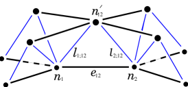
Figure 1: The construction of a new spin network under Rule 1.

Two of the nodes of $\Gamma_{1}$, $n_{i}^{\prime}$ and $n_{j}^{\prime}$ will be connected by an edge $e^{\prime}_{ij}$ in $\Gamma_{1}$ if the edges $e_{i}$ and $e_{j}$ were incident on a common node $n_{\alpha}$ in $\Gamma_{0}$. The result is that the new graph $\Gamma_{1}$ is related to the old one by a kind of duality in which edges go to nodes and nodes go to complete graphs, which are graphs in which each node is connected to every other node. (See Figure 2).

Figure 2: Two steps in the evolution of a trivalent spin network, following first Rule 1, then Rule 2.

The result of this rule is a spacetime spinnetwork ${\cal G}_{01}$ bounded by the two ordinary spin networks $\Gamma_{0}$ and $\Gamma_{1}$ whose nodes are connected by a set of null edges. In general a spacetime spin network (or spacetime net, for short) will consist of a set of $N$ ordinary spin network, $\Gamma_{i}$, $i=0,1,...,N$, together with a set of null edges that join nodes of $\Gamma_{i}$ to nodes of $\Gamma_{i+1}$. We may also have need to refer to the graph made only of the null edges that join the spinnets, which we call the internet.

The motivation for this construction is the following: We imagine that the initial spin network $\Gamma_{0}$ is embedded in a spacelike slice $\Sigma_{0}$ of a four dimensional spacetime ${\cal M}$, such that the edges correspond to spacelike geodesics. (This imaginary embedding is only for motivation, once the rules are established it plays no role.) Each node $n_{i}$ of $\Gamma_{0}$ emits a light signal which evolves into its future lightcone in $\cal M$. For each $n_{i}$ and $n_{j}$ connected by an edge $e_{ij}$, there will be an event at which the light rays from those nodes, each traveling in the direction of the geodesic to the other edge, first meet. This event corresponds to the new node $n^{\prime}_{ij}$ and the null edges $l_{i;ij}$ and $l_{j;ij}$ correspond to the null rays emmited by $n_{i}$ and $n_{j}$ that met at $n_{ij}^{\prime}$. (See Figure 3.)

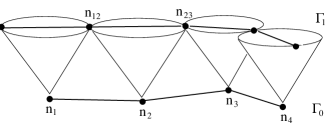
Figure 3: The new nodes represent events defined by meeting of causal processes.

For each edge $e_{ij}$ of $\Gamma_{0}$ we then have an event to the future, $n_{ij}^{\prime}$. These are the nodes of the successor spin network $\Gamma_{1}$; we may imagine that they are embedded in a second two dimensional surface $\Sigma_{1}$ embedded in $\cal M$ to the future of $\Sigma_{0}$. (See Figure 3). We will assume that this surface can be chosen so that it is spacelike, this corresponds to the fact that in the construction there are no null edges that connect nodes in the same $\Gamma_{i}$. (Of course whether this can be done in an arbitrary spacetime $\cal M$ given an arbitrary spacetime metric $g_{ab}$ is a dynamical question, but as we are specifying the dynamics and the spacetime metric in terms of the discrete structure there is no loss of generality in assuming this. To put this another way, as the embedding is only for motivation, we need only that it is possible to choose some metric $g_{ab}$ such that the surface $\Sigma_{1}$ is spacelike.)

The basic idea of the construction is that the rule for assigning edges that connect the new nodes $n_{ij}^{\prime}$, as well as the rules for assigning amplitudes to labelings of the edges must satisfy a discrete causal principle. This causal principle is stated in terms of a discrete causal structure, which is specified by the null edges. Thus, each node in the spacetime net $\cal G$ has a future and past light cone, which is gotten by following null edges from it to the past or the future. Two nodes of a spacetime net $\cal G$ will be said to be causally connected if and only if there is a path of future pointing null edges, that link one to the other. The causal past or future of a node then consists of all nodes to which it is causally connected by a path of null edges going into the past or future, and all edges such that both ends are in the causal past or future of it. The causal past or future of an edge is the union of the causal past or future of its two ends. Given this structure we propose a principle of discrete causality which says that:

• The information about which other nodes a node is connected to, as well as the colorings of a node or edge, can only be determined by information in its causal past, except that the assignment of amplitudes may induce correlations among two edges that share a common node.

In this definition, the information available at a node is its color and the number and colors of the edges incident on it; the information available at an edge is its color and the colors of its ends.

Thus, which other nodes $n^{\prime}_{kl}$ a given node $n^{\prime}_{ij}$ may be connected to in $\Gamma_{1}$ can be determined only by information that is in the backwards light cone of $n^{\prime}_{ij}$, which will be denoted ${\cal C}_{n^{\prime}_{ij}}^{-}$ (See Figure 4.) In addition to this we will make a second assumption, which is that the dynamics be as local in time as possible. This means that the information necessary to specify the connectivity of a node in a successor spinnet $\Gamma_{1}$, or the color of one of its edges should depend directly only on information available in the intersection of the backwards light cone of that node or edge with the previous spinet $\Gamma_{0}$, and not on any information from earlier spin networks.

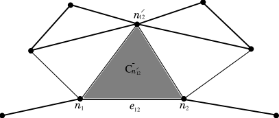
Figure 4: The backwards light cone ${\cal C}_{n^{\prime}_{12}}^{-}$ of the node $n^{\prime}_{12}$.

The only part of $\Gamma_{0}$ that is in ${\cal C}_{n^{\prime}_{ij}}^{-}$ consists of the two nodes $n_{i}$ and $n_{j}$ and the edge $e_{ij}$ that joins them. (See Figure 4). Therefore all the information that determines who $n^{\prime}_{ij}$ is connected to and how it is labeled must be available there. This information consists of the labeling of $e_{ij}$, the information about which other edges of $\Gamma_{0}$ are incident on $n_{i}$ and $n_{j}$ and the labelings of those edges.

The simplest rule for connecting the nodes of $\Gamma_{1}$ consist with this discrete causality principle is the one we have given: two nodes are connected if the edges they correspond to in $\Gamma_{0}$ were incident on the same node.

We may note that no instruction is given for how the new spinnet $\Gamma_{1}$ may be embedded in a two dimensional manifold $\Sigma_{1}$. The spinnets used here are to be considered to be purely combinatorial structures, which come with no such embedding information. This is true as well for the spacetime spinnets ${\cal G}$. While we may use a picture in which $\cal G$ is embedded in some $2+1$ dimensional spacetime, this is only to allow us to use our intuition about causal structure to motivate the rules and principle of causality for the discrete construction. Once the construction is specified the notion of a spacetime continuum may be recovered only in the case that the dynamics shows critical behavior that allows us to define a continuum limit.

We have yet to specify the labelings of the nodes and edges of $\Gamma_{1}$. To do this let us recall that the original graph $\Gamma_{0}$ was trivalent. Then each node in the successor graph $\Gamma_{1}$ is four valent (See Figure 2). There is a natural choice of assignment of its state, which is that it is given by a virtual spin network in which the four valent node is decomposed into two trivalent nodes joined by a virtual edge parallel to $e_{ij}$ (See Figure 5). The virtual edge can then be colored by the same spin that labels $e_{ij}$.

Figure 5: The labeling of a new four valent nodes is gotten from that of the edge that gave rise to it. A dotted circle around a subgraph means that it is virtual.

There is no natural unique assigment for the labelings of the edges of $\Gamma_{1}$. Instead we will assign a complex amplitude ${\cal A}_{0\rightarrow 1}$ to each set of labelings of the edges of $\Gamma_{1}$, given the labelings of $\Gamma_{0}$. To see how to do this we note that there are two restrictions on the labelings and amplitudes. The first is that the labelings of the edges of $\Gamma_{1}$ must be consistent with the labelings on the nodes, which have already been determined. This condition is easily stated in terms of the decomposition of each node of $\Gamma_{1}$ into trivalent virtual nodes, each then has one incident virtual edge whose labeling has been determined from the previous paragraph and two real edges whose labeling must be determined, the possible labelings of the real edges must then be chosen so that the addition of angular momentum is satisfied at each virtual node.

The second restriction is the principle of causality. The discrete backwards lightcone of an edge $e^{\prime}_{(ij)(ik)}$ in $\Gamma_{1}$ contains a subgraph $\gamma$ of $\Gamma_{0}$ that contains the nodes $n_{i}$, $n_{j}$ and $n_{k}$ as well as the two edges $e_{ij}$ and $e_{ik}$. (See Figure 6).

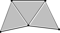
Figure 6: The backwards light cone of an edge.

Therefore the information relevant for the labeling of $e^{\prime}_{(ij)(ik)}$ must be taken from only information available at those nodes and edges. A perscription consistent with this restriction is the following. Consider the three pairs of edges incident at a node $n_{i}$, which are $e_{ij},e_{ik}$ and $e_{il}$. These have labelings that for simplicity we may denote by $i,j,k$ and $l$. The node $n_{i}$ gives rise by the evolution rule to a triangle whose edges are (See Figure 7), $e^{\prime}_{(ij)(ik)}$, $e^{\prime}_{(ij)(il)}$ and $e^{\prime}_{(ik)(il)}$. For simplicity let us denote these edges simply by $e^{\prime}_{m}$, $e^{\prime}_{n}$ and $e^{\prime}_{p}$ and their labeling by $m,n$ and $p$, respectively. The simplest assumption consist with the restriction of causality is that there is an amplitude $J(mnp;jkl)$ for each choice of labeling of the new edges $mnp$, given the labelings of the old edges $ijk$.

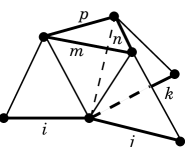
Figure 7: The evolution of a trivalent node.

Figure 8: The label of a null edge is the same as that of the spacelike edge that gave rise to it.

To see what conditions this amplitude $J(mnp;jkl)$ must satisfy, let us note that it corresponds naturally to a tetrahedron in the spacetime network ${\cal G}_{01}$. One thing we have not done is labeled the null edges. However, there is a natural way to do this, which is to note that each edge $e_{ij}$ in $\Gamma_{0}$ gives rise to two null edges $l_{i;ij}$ and $l_{j;ij}$ in the spacetime network. The intersections of their causal pasts with $\Gamma_{0}$ consists only of the edge $e_{ij}$ and the two nodes it joins. However, as the nodes of $\Gamma_{0}$ are assumed to be trivalent and, hence, unlabeled, the only information a labeling of the two null edges could depend is the color of the original edge. Therefore, the only natural assumption is that the null edges are labeled with the same coloring as the edge it came from (See Figure 8 ).

There is then a tetrahedron ${\cal T}_{i}$ in ${\cal G}_{01}$ corresponding to each node $n_{i}$ of the original spin network $\Gamma_{0}$ (see figure 9). It contains three null edges, whose labelings are known and three new spacelike edges which are part of the new spin network $\Gamma_{1}$. There is then an amplitude $J(mnp;jkl)$ associated to each such tetrahedron. This amplitude must be consistent with a subset of the symmetries of the tetrahedron, which are those that do not mix the null and spacelike edges.

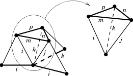
Figure 9: The spacetime tetrahedron used to determine the labels $m,n,p$ on the edges of a triangle that is the future evolution of a trivalent node.

The total amplitude will then be taken to be

$${\cal A}_{0\rightarrow 1}=\prod_{i}J(mnp;jkl)$$ (1)

where the product is over all nodes $n_{i}\in\Gamma_{0}$.

The choice of a function $J(mnp;jkl)$ corresponds to the choice of dynamics. The parameter space of the theory then consists of the possible functions $J(mnp;jkl)$ of the six spins in Figure 9 that is invariant under rotations in space of the spacelike triangle. Within this space of possible theories is a special one, based on the choice,

$$J(mnp;jkl)={\cal T}[mnp;jkl]$$ (2)

where ${\cal T}[mnp;jkl]$ is the “tetrahedronal symbol”, which is a $6j$ symbol normalized so that it has all the symmetries of the tetrahedron[35]. The ${\cal T}[mnp;jkl]$ has more symmetry than we need and is also special in that it satisfies the $6j$ symbol identities. It is possible that with this choice the theory corresponds to a $2+1$ dimensional topological quantum field theory, but that has so far not been shown.

3.2 Rule 2

We might just apply Rule 1 over and over again, but the result would be that each successor spin network has nodes of higher and higher valency. (This is easy to see, if each node of $\Gamma_{n}$ has valence $P$, each node of $\Gamma_{n+1}$ will have valence $2(P-1)$.) To prevent this from happenning we need a second rule that lowers rather than raises the valence of the nodes. There is a natural choice for such a rule which is the following. Recall that each higher-than-trivalent node $n_{i}^{\prime}$ has associated to it a state $|\eta\rangle$ in a finite dimensional state space. This space, ${\cal V}_{n_{i}}$, is spanned by a basis of states $|\gamma\rangle$, each of which can be represented as an open spin network whose ends are the edges incident on $n_{i}$ connected to each other through a set of virtual trivelent nodes and edges. In the case of a four valent node, the space may be labeled ${\cal V}_{4,ijkl}$, where $i,j,k$ and $l$ are the spins of the four edges incident on it.

A four valent network can be labeled by inserting a virtual edge, as we have already indicated in Figure 5. For each node in $\Gamma_{1}$ there is a natural way to split it, parallel to the edge that gave rise to it. Corresponding to that we may evolve the network by splitting it, so that the virtual node becomes real (See the middle term in Figure 10.)

Figure 10: The three ways a node splits under Rule 2.

The effect of this shown in Figure 11.

Figure 11: The effect of the three splittings in Rule 2.

The new edge created is labeled by the same label $m$ that was on the edge in $\Gamma_{0}$ that gave rise to the node in $\Gamma_{1}$.

However, there are two other ways that the node could be split into a pair of trivalent nodes. Let us call the first way the “s channel”, and the other two the “t channel” and “u channel”, by analogy to scattering theory (See Figure 10). Associated with each there are states in ${\cal V}_{4,ijkl}$, which may be labeled $|t;n\rangle$ and $|u;p\rangle$. (The original state shown in Figures 5 is then called $|s;m\rangle$.) Each of these may be split, giving rise to two new trivalent nodes and a new edge, which has the same label as the virtual edge it came from.

Rule 2 may then be stated as follows:

• $\Gamma_{2}$ consists of a sum of terms which are gotten from $\Gamma_{1}$ by splitting each four valent node in each possible way corresponding to the $s,t$ and $u$ chanel states in the spaces ${\cal V}_{4,ijkl}$. The $s$ channel split is multiplied by an amplitude $a$. Each $t$ channel split is multiplied by an amplitude $b\langle t;n|s;m\rangle$ and each $u$ channel split by $c\langle u;p|s;m\rangle$ where $|a|^{2}+|b|^{2}+|c|^{2}=1$.

  For each spin network $\Gamma_{2}$ produced by the rule the amplitude ${\cal A}_{\Gamma_{1}\rightarrow\Gamma_{2}}$ is then the product of these factors for every four valent node that is split.

• In each term each of the two new nodes are then connected to the original node by a new null edge, as in Figure 10. The two null edges created may be labeled by the same label as the new spacelike edge associated with them.

• Rule 2 also preserves all of the edges of $\Gamma_{1}$, which appear in $\Gamma_{2}$, with the same labels.

  We may note that there is freedom in the specification of Rule 2, associated with the choices of the amplitudes $a,b,c$ for the $s,t$ and $u$ channels. Unless they are needed, however, it is simplest to set them equal so that $a=b=c=1/\sqrt{3}$.

3.3 Combining the two rules: the transition law

The effect of Rule 2 is to make the resulting graph $\Gamma_{2}$ trivalent. If we apply the two rules in succession, starting with any initial spinnet, we generate a discrete causal graph ${\cal G}$ which is foliated by spin networks that are alternatively trivalent and four valent (here and elsewhere in this paper, valence counts only spacelike edges and ignores the null edges). The nodes of these spinnets are connected by null edges in the following way: each trivalent node has one null edge going into the past and three going into the future. Each four valent node has two null edges going into the past and two going into the future.

We may then state the dynamics of quantum gravity in the following form: Given two trivalent spin networks $\Gamma_{i}$ and $\Gamma_{f}$ we construct the amplitude ${\cal A}_{\Gamma_{i}\rightarrow\Gamma_{f}}$ for the first to evolve to the second. We consider all causal spacetime nets ${\cal G}$ consistently built by the alteration of the two rules which have $\Gamma_{i}$ as the zeroth spin network and $\Gamma_{f}$ as the last. $\cal G$ will have an odd number $L_{\cal G}$ of component spinnets, $\Gamma_{I}$. We then have

$${\cal A}_{\Gamma_{i}\rightarrow\Gamma_{f}}=\sum_{\cal G}\prod_{I=0}^{L_{\cal G}-1}{\cal A}_{\Gamma_{I}\rightarrow\Gamma_{I+1}}$$ (3)

where the sum includes the sums over all the allowed colorings and the amplitude is defined alternatively in terms of Rule 2 or Rule 1.

Figure 12: A piece of a spacetime network with the fourth level under construction. The lightcones symbolize the null edges formed by Rule 1.

Thus we have achieved our goal, which is an amplitude for evolution of spinnetworks in terms of a sum over intermediate four dimensional “spacetime nets”, whose construction defines a discrete version of causal structure that is then obeyed by the rule for assigning amplitudes.

3.4 Interpretation in terms of timelike surfaces

The spacetime nets $\cal G$ defined by the evolution rules contain sets of “timelike” surfaces. Examples of these are triangles defined by Rules 1 and 2, which we see shaded, respectively, in Figures 4 and 10, and a set of squares which are created by the evolution of edges that are preserved by Rule 2. The former have two null edges and one spacelike edge while the latter have two of each. The labelings may be extended to labelings of these timelike surfaces by assigning to each triangle or square the labelings of its spacelike edges (the two spacelike edges of each square have the same labels.) This creates two kinds of surfaces that share common labels: diamonds with four null edges and hexagons with six null edges. These timelike surfaces may be considered to be the primary objects out of which the spacetime nets are constructed. The result is a theory in which the amplitude for a spin network to evolve to another one is given by a sum over terms, each of which consists of a set of labeled timelike surfaces. This is the same as in the formulation of Reisenberger and Rovelli [33] and in topological quantum field theory [30].

4 The $3+1$ dimensional theory

We can raise the spatial dimension from $2$ to $3$ by making several modifications in the structure we just defined.

• We raise the valence of each node of the initial spin network $\Gamma_{0}$ from $3$ to $4$. Most combinatorial four valent graphs are not planar, but they can each be embedded in a three dimensional manifold.

• Each node of the initial four valent network must now be labeled, by inserting a virtual trivalent graph as described in [11]. Furthermore, if we consider possible embeddings of $\Gamma$ into a three manifold $\Sigma$, generic nodes will contribute to the volume of $\Sigma$.

• The successor network constructed by Rule 1 will consist of six valent nodes (Figure 13). The complete graphs, corresponding to the triangles of the $2+1$ theories, are now tetrahedra. There is thus one tetrahedra ${\cal T}_{n}$ in $\Gamma_{1}$ corresponding to each node $n$ of $\Gamma_{0}$. Associated to each such node of $\Gamma_{0}$ there is then a four simplex, consisting of the spacelike tetrahedra ${\cal T}_{n}$ in $\Gamma_{1}$ just described and the four null lines that connect its nodes to $n$. We shall call this ${\cal S}_{n}$.

  As before, the null lines in ${\cal S}_{n}$ are labeled by the spins of the $4$ edges incident on $n$. $n$ is also labeled. We need to prescribe an amplitude for each assignments of labelings to the four nodes and six edges of ${\cal T}_{n}$. This will be called ${\cal J}^{15}$ as it is a function of $15$ labels, corresponding to ten edges and five nodes of ${\cal S}_{n}$.

  The dynamics are then given by a choice of ${\cal J}^{15}$. As in the $2+1$ dimensional case, the space of such functions is the parameter space of the theory. The simplest choice is to take ${\cal J}^{15}$ equal to the $15j$ symbol[30], which, as in the $2+1$ dimensional case, is associated with topological quantum field theories.

• To complete the specification of Rule 1 we must say how the new six-valent nodes created are labeled. There is a natural prescription associated with this that preserves the principle of causality. Each new six valent node $n^{\prime}_{12}$ may be virtually split into two four-valent nodes, joined by a virtual edge that is parallel to the edge $e_{12}$ it came from. Let the label of $e_{12}$ be $m$. This edge joins two nodes, $n_{1}$ and $n_{2}$. Each is in a state $|\Psi_{1}\rangle$ and $|\Psi_{2}\rangle$ in their corresponding spaces ${\cal V}_{4}$, each of which may be describe by a superposition of virtual trivalent graphs. We may associate to the node the state in the associated space ${\cal V}_{6}$ which is described by the states $|\Psi_{1}\rangle$ and $|\Psi_{2}\rangle$ associated with $n_{1}$ and $n_{2}$ joined by a virtual edge labeled by $m$. That is, we simply read the subgraph consisting of $n_{1}$, $n_{2}$ and $e_{12}$ as describing a state in the space ${\cal V}_{6}$ associated to the new node.

  

  Figure 13: The labeling of a six valent node in the $3+1$ theory: The subgraph indicated is the state of the new node.

• Rule 2 then must break each $6$ valent node of $\Gamma_{1}$ back down into a pair of four valent nodes. As in the $2+1$ dimensional case, we will sum over the different ways of doing this, with an amplitude given by the inner product between the state $|m\rangle$ given by the labeling on the six valent node, $m$, and the state given by the pair of four valent nodes in $\Gamma_{2}$, with their labelings. There are $20$ ways to make the split, each of which produces a pair of four valent nodes, each separated by new edge. Each of the two four valent edges must then be labeled as well; a basis of states here must be labeled by a virtual edge. Associated with each way of splitting the six valent node we then have a state in its ${\cal V}_{6}$, which we may call $|p\rangle$. The (unormalized) amplitude for each split will then be given by $\langle p|m\rangle$.

By comparing the two sets of rules we can see several reasons why the first is associated with $2+1$ theory and the second with $3+1$. 1) In the first case the spatial spin networks are planar, in the second, generally not. 2) The spacetime objects which represent the elementary discrete future null cones are three and four simplices, repsectively. 3) The corresponding simplest choices for amplitudes in each case are the $6j$ and $15j$ symbols, which are the amplitudes associated with the simplest versions of $3$ and $4$ dimensional topological quantum field theory. 4) All the nodes of the $3+1$ dimensional theory have non-zero quanta of three dimensional volume generically.

5 $1+1$ dimensional models

We have defined a family of discrete quantum theories of gravity in $2+1$ and $3+1$ dimensions, each of which is described by a choice of a function of the labelings on a tetrahedron or four simplex, respectively. Given a choice of these functions, we have a complete perscription for a path integral for quantum gravity. However, it is not simple to work out its consequences and investigate questions such as the existence of a classical limit. It is then useful to construct an analogous model in 1+1 dimensions, which may be analyzed more easily.

5.1 A first $1+1$ dimensional model

A spatial state of this consists of a circle broken up into $N$ segments by $N-1$ nodes. The segments are labeled by elements of some set of colors $\cal L$. These will not be interpreted as spins, as then conservation of angular momentum would restrict them to be all the same (See Figure 14).

Figure 14: A $1+1$ dimensional model.

In this case there is only one evolution rule, which is essentially Rule 1 of the higher dimensional case. Each node emits two null edges, one going to the left and one to the right. Each edge $e_{i}$ then gives rise to a new node $n^{\prime}_{i}$. This can be interpreted as the event where the right moving light ray from the left edge of $e_{i}$ meets the left moving light ray from its right edge. Each old node is then replaced by a new edge $e_{i}^{\prime}$, with a new labeling $l$. (See Figure 14). There must be a rule which gives an amplitude $J(j,k;l)$ for the new edge $e_{i}^{\prime}$, given the labelings of the two edges that were adjacent to the node that gave rise to it.

The resulting $1+1$ dimensional spacetime net can also be interpreted in terms of labeled timelike surfaces, which in this case are all diamonds. The amplitude $J(j,k;l)$ is then assigned to each triple of neighboring diamonds, in which the $j$ and $k$ are the labels of the diamond just to the past of the diamond labeled by $l$ (See Figure 14).

Given a choice of the amplitude $J(j,k;l)$ we then have a complete rule for the amplitude of the evolution of states. Given an initial state $\Gamma_{i}$ and a final state $\Gamma_{f}$, each given by a circle of labeled segments. Then the amplitude for the transition is given by

$${\cal A}_{i\rightarrow f}=\sum_{\cal G}\prod J(i,j;k)$$ (4)

where the sum is over all spacetime nets $\cal G$ whose boundary $\partial{\cal G}=\Gamma_{i}+\Gamma_{f}$. and for each spacetime net the product is over all triples of nearest neighbor diamonds.

Figure 15: A history for the first kind of $1+1$ dimensional model.

We may give two examples of such nearest neighbor rules. First, we can model the system as a lattice gauge theory. In this case $i,j,k,...$ are elements of some group $G$ and $J(i,j;k)=exp[\imath\beta Tr_{\rho}[ijk]]$ where the trace is taken in a representation $\rho$. The resulting theory is a kind of anisotropic $1+1$ dimensional lattice gauge theory.

A second model is a kind of Potts model in which $i,j,k\in Z_{n}$ and $J(j,k;l)=exp[\imath\beta|j+k-2l|^{2}]$.

5.2 Directed percolation model

We can describe a third kind of $1+1$ dimensional model by doing the following. Represent each diamond as a site of a $1+1$ dimensional lattice, and represent each future pointing causal link between diamonds as a null edge between the corresponding nodes (see Figure 16). Call the resulting $1+1$ dimensional spacetime lattice, consisting of only of the nodes and the null edges, $\Delta$. (This is what we called the internet before). There is a form of the theory in which the dynamical variables are associated only with the null edges. In the simplest case, each null edge $l_{ij}$, connecting nodes $i$ and $j$ is either on or off. These states may be represented by either the presence of absence of an arrow. A history of the system is given by a choice of on or off for each null edge in $\Delta$. It may be represented by a graph $\rho$ gotten by removing from $\Delta$ those null edges which are off (see Figure 17).

Figure 16: The lattice of the percolation model.

Figure 17: A history in the percolation model.

The evolution rule will consist of an amplitude ${\cal A}_{n}$ for each node $n$ which is a function of the four null edges incident on $n$, the two that come from the past and the two that go out to the future. We will not put any condition on these rules, except to impose that the amplitude that one or both arrows in the future of a node $n$ are on must be zero in the case that both incoming arrows are off. A specification of the amplitude ${\cal A}_{n}$ is a function of the sixteen possible states of the two incoming and two outgoing arrows.

It is interesting to note that this theory is closely related to three kinds of theories that have been studied before. First, each history $\rho$ is a causal set. We may then seek to embed it in a $1+1$ dimensional manifold $\Sigma$ with metric $g_{ab}$ preserving both the causal structure and the spacetime volume (where we follow ’tHooft’s suggestion that the spacetime volume of a region is the number of nodes in Planck units[3]).

Second, this theory is closely related to a class of statistical models known as directed percolation. There are a number of such models[31]. In the simplest, each arrow may be on or off with an independent probability $p$. In more sophisticated models, there are probabilities associated to each choice of in arrows and out arrows, subject only to the restriction that the probability for out arrows to be on is zero if all both in arrows are off. This model then corresponds to a special case of the quantum gravity model we have described in which the amplitudes are all real and positive so that they sum according to the rules of classical probabilities.

Interestingly enough, both of these models have critical behavior, which corresponds to percolation[31]. While they are different, they are in the same universality class, which is to say that their critical behavior is identical. A large number of other statistical mechanics models fall into the same universality class[31].

The third kind of closely related theories are binary networks, or cellular automata, in which there is a definite rule by which the outgoing arrows are determined as a function of the incoming arrows. This case is also a special case of our model in which the amplitudes are treated as classical probabilities. Within this class of models are also some that have critical behavior. There is even a class of such models with self-organized critical behavior[32].

Directed percolation models exist and have non-trivial critical behavior for all dimensions up to $3+1$. It is interesting to note that corresponding to each such theory one gets a statistical theory of the corresponding causal sets. Thus, this is a connection that may be fruitfully pursued. The most important question to understand is whether the theories with complex amplitudes rather than classical probabilities have critical behavior. It would be especially interesting if such theories were to have self-organized critical behavior.

6 Conclusions

We have described here a class of theories for $1+1$, $2+1$ and $3+1$ dimensional quantum gravity. Each of them gives a discrete path integral for the amplitude for any spin network state $|\Gamma_{initial}\rangle$ to evolve to a final state $|\Gamma_{final}\rangle$. In each case the dynamics are specified by giving a complex function, $J(i,j,...)$ of the labelings of a $d+1$ dimensional simplex. The possible such functions consistent with the symmetries of the simplex that do not mix spacelike and null edges thus comprise the parameter space of this class of theories. In $2+1$ and $3+1$ there are natural choices for these functions, which are the normalized $6j$ and $15j$ symbols respectively. We may conjecture that these choices lead to a topological quantum field theories, given the closeness of the theory to them in that case, but this has yet to be shown. What needs then to be done is to explore the behavior of the theory given different choices for the $J$’s. Those choices that have critical behavior will be candidates for quantum theories of gravity. If they exist they will be theories that are finite and discrete at the Planck scale, are based on the kinematical structures discovered by canonically quantizing general relativity and have a continuum limit in which classical spacetime is reconstructed by making use of the causal relations of the spacetime networks. In these cases the continuum limit should be described by the Einstein’s equations, in the limit of large radius of curvature.

We believe that the crucial problem to be studied in this class of theories is the existence of critical behavior, as this is necessary for the existence of a continuum limit. We find especially interesting the fact that the spacetime networks have two structures, associated with spin networks and causal sets. Each theory by itself has failed to have enough structure to ensure the existence of a good continuum limit, we hope that by using both of them, it will be possible to investigate the question of the existence of the continuum limit.

Another related issue is the possibility that the critical behavior of these theories will be self-organized. At least philosophically, this would be attractive as it would save us from the problem of having to believe that the existence of a classical limit for a quantum theory of gravity depends on the fine tuning of some parameters.

To investigate these kinds of questions, we find the relationship with directed percolation models very promising. In particular, the fact that every configuration of a directed percolation model is a causal set means that each directed percolation model is at the same time a statistical theory of discrete spacetime geometry. As there exist such models in $d+1$ dimensions, for $d$ at least up to $3$, this gives us a rich new class of models of dynamical spacetime geometry, which are already set up to study the key problem of the existence of the continuum limit.

This connection raises further interesting questions, which deserve study. Among them are whether there is a universality class of quantum directed percolation, in which the histories are weighed by complex amplitudes rather than real probabilities.

A related line of attack is to construct a renormalization group transformation on the space of such theories. One approach, which preserves both the kinematical interpretation of the spin network states and the causal properties of the spacetime networks is presently under development[37].

Other avenues of attack concern the relationship of the class of theories we propose here with topological quantum field theories in $3$ and $4$ spacetime dimensions. As mentioned above, we suspect that particular choices of the dynamical parameters, in which the $J$’s are taken proportional to $6j$ or $15j$ symbols, respectively, are closely related to the respective topological quantum field theories. If this is the case then it may provide an avenue of attack on the renormalization group behavior of theories which are close to the $TQFT$’s. These theories are also likely to be closely related to the Euclidean Reisenberger-Rovelli models.

Finally, at the classical level the theories we describe may be related to null strut regge calculus[38].

Before closing this paper we would like to elaborate on several of these issues in more detail.

6.1 Causal sets and the classical limit

To see how the causal set structure may play a role in the classical limit let us ignore for a moment the additional structure associated with the spin networks. Considering only its causal structure, a spacetime network consists of a set of points together with causal relations. These causal relations are coded entirely in the null edges; the causal structure is completely independent of the spinnets that tie together nodes on a single “spatial slice”. It is coded entirely in what we called “the internet”.

Given any causal set, we can ask if it embeds in a spacetime manifold, $\cal M$ with spacetime metric, $g_{ab}$, such that the nodes are mapped to points of $\cal M$ such that the causal structure is preserved. Even if it does the metric and embedding will not be unique, but we can ask if all metrics and embeddings of a given spacetime net share an averaged casual structure. That is, is there some coarse grained metric $\tilde{g}_{ab}$ defined by averaging the metrics $g_{ab}$ over many Planck volumes, such that all embeddings of the spacetime net agree? If so, then we can say that the spacetime net has a classical limit, given by the common average, $\tilde{g}_{ab}$.

The spacetime metrics $g_{ab}$ will be defined up to conformal structure. It follows that the averaged metric will also be only determined up to conformal structure, at least as long as the conformal transformations are sufficiently slowly varying.

To fix the conformal class of the averaged metric will require additional information. This information has to do with the volume of spacetime regions. However, this information is likely provided by the other information in the spin networks. First of all, the spatial volumes of regions of spatial slices are fixed by the labels of the nodes and edges of each spin network. It remains to fix the lapse functions. However, these are not free, as they are fixed by the causal relations. (The implications of this are discussed below.) Thus, it is likely that the spin networks provide sufficient additional information to allow the reconstruction of the conformal factor. The details of how the causal structure and spin network structures may interact to determine an embedding in a classical geometry remain to be worked out. But it seems promising that by combining the two structures we have a possibility of a kind of classical limit that is not available for Euclidean quantum gravity.

6.2 Time reversal invariance and noninvariance

It is evident that the rules we have defined here are not time reversal invariant, for example the number of nodes in each spin network $\Gamma_{i}$ generally increases with $i$. If it were shown to be necessary, it would be possible to remedy this by simply including additional rules which are the time reversals of Rules 1 and 2. However, there are several reasons to investigate the theory as is. As we have argued, if there is critical behavior the classical Einstein’s equations must govern the classical limit, so that time reversal invariance may be restored at the classical level. Time reversal invariance may in fact play a role in the establishment of the continuum limit, as it is a feature of directed percolation models that seem related to those we study here. For one thing, we would like a satisfactory theory to have a continuum limit that was a consequence of self-organized critical behavior, and such behavior is normally found in the domain of non-equilibrium, time reversal non-invariant systems. Finally, there are a number of independent arguments that suggest that quantum gravity either may be, or must be time reversal non-invariant.

6.3 Spacetime diffeomorphism invariance

The reader may object that if the dynamics is not generated by a constraint we have not imposed all of the gauge invariance of the theory. However, we may note that the rules we described do not allow a freedom to continuously deform the spatial slices. If we imagine that the spacetimenet is embedded in a background $d+1$ dimensional spacetime ${\cal M},g_{ab}$ preverving the discrete light cone structure then it will not be possible to vary the embeddings of the spatial slices independently. This is because, once the embedding of the first slice is picked, the second, which is constructed by Rule 1, is determined by the intersection of null cones.

Thus, the rules we have given fix the gauge freedom corresponding to the Hamiltonian constraint. An important question is then whether the full spacetime diffeomorphism invariance is recovered as a gauge freedom of the effective action in the continuum limit. As the relationship with the classical geometry will go through the poset construction, it is likely that this is the case, as the correspondence between the exact discrete spacetimenet and the approximate continuum description uses only the causal structure, which is spacetime diffeomorphism invariant.

If this is the case, then the effective classical theory that emerges will satisfy a Hamiltonian constraint, as that will be a reflection of the invariance of the effective action under spacetime diffeomorphisms. Thus, the Hamiltonian constraint will be recovered in the classical limit, even if it is not put in at the fundamental level of the theory.

We may note that this implies that the discrete theory may have a notion of time and evolution that is not coded in its continuum limit. We believe that this possibility that discreteness may resolve the problem of time in quantum gravity is significant, and should be investigated in its own right.

References

- [1] R. Penrose, in Quantum Gravity, an Oxford Symposium ed. C. J. Isham, R. Penrose and D. W. sciama, Clarendon Press, Oxford, 1975.
- [2] L. Bombelli, J. Lee, D. Meyer and R. D. Sorkin, Spacetime as a causal set Phys. Rev. Lett. 59 (1987) 521.
- [3] G. ’t Hooft, Quantum gravity: a fundamental problem and some radical ideas. Cargèse Summer School Lectures 1978. Publ. “Recent Developments in Gravitation”. Cargèse 1978. Ed. by M. Lévy and S. Deser. Plenum, New York/London, 323; Quantization of Space and Time in 3 and in 4 Space-time Dimensions, Lectures held at the NATO Advanced Study Institute on “Quantum Fields and Quantum Space Time”, Cargèse, July 22 – August 3, 1996. gr-qc/9608037; The scattering matrix approach for the quantum black hole: an overview. J. Mod. Phys. A11 (1996) pp. 4623-4688. gr-qc/9607022.
- [4] A.A. Ashtekar, Phys. Rev. Lett. 57 (1986) 2244; Phys. Rev. D36 (1987) 1587
- [5] T. Jacobson and L. Smolin, Nucl. Phys. B 299 (1988).
- [6] C Rovelli L Smolin: Phys Rev Lett 61 (1988) 1155; Nucl Phys B133, 80 (1990).
- [7] R Gambini A Trias: Phys Rev D23 , 553 (1981); Lett al Nuovo Cimento 38, 497 (1983); Phys Rev Lett 53, 2359 (1984); Nucl Phys B278, 436 (1986); R Gambini L Leal A Trias: Phys Rev D39 , 3127 (1989); R Gambini: Phys Lett B 255, 180 (1991)
- [8] L Smolin: in Quantum Gravity and Cosmology, eds J Pérez-Mercader et al, World Scientific, Singapore 1992.
- [9] A. Ashtekar , Non-perturbative canonical gravity. Lecture notes prepared in collaboration with Ranjeet S. Tate. (World Scientific Books, Singapore,1991).
- [10] C. Rovelli, Classical and Quantum Gravity, 8 (1991) 1613-1676.
- [11] C. Rovelli and L. Smolin, “Spin networks and quantum gravity” gr-qc/9505006, Physical Review
- [12] C. Rovelli and L. Smolin Discreteness of area and volume in quantum gravity Nuclear Physics B 442 (1995) 593. Erratum: Nucl. Phys. B 456 (1995) 734.
- [13] R. Loll, Phys. Rev. Lett.
- [14] A. Ashtekar and J. Lewandowski, ”Quantum Geometry I: area operator” gr-qc/9602046.
- [15] R. DePietri and C. Rovelli, Geometry eigenvalues and scalar product from recoupling theory in loop quantum gravity, gr-qc/9602023, Phys.Rev. D54 (1996) 2664; Simonetta Frittelli, Luis Lehner, Carlo Rovelli, The complete spectrum of the area from recoupling theory in loop quantum gravity gr-qc/9608043
- [16] T. Thiemann, Closed formula for the matrix elements of the volume operator in canonical quantum gravity Harvard preprint, 1996, gr-qc/9606091gr-qc/9601038 .
- [17] J. Lewandowski, ”Volume and quantization” gr-qc/9602035.
- [18] R. Borissov, S. Major and L. Smolin, The geometry of quantum spin networks gr-qc/9512043, Class. and Quant. Grav. 12 (1996) 3183.
- [19] R. Borissov, Ph.D. thesis, Temple, (1996).
- [20] T. Thiemann, A length operator in canonical quantum gravity Harvard preprint 1996, gr-qc/9606092
- [21] C Rovelli L Smolin: Phys Rev Lett 72 (1994) 446
- [22] R. Borissov, Graphical evolution of spin network states, gr-qc/9605.
- [23] T. Thiemann, Quantum spin dynamics I, Harvard preprint (1996), gr-qc/9606089.
- [24] T. Thiemann, Quantum spin dynamics II, Harvard preprint (1996), gr-qc/9606090.
- [25] L. Smolin, The classical limit and the form of the hamiltonian constraint in non-pertubative quantum gravity CGPG preprint, gr-qc/9609034.
- [26] S. Weinberg, General Relativity: An Einstein Centenary Survey in S. W. Hawking and W. Israel, Cambridge University Press, 1979. eds.
- [27] L. Smolin A fixed point for quantum gravity Nucl. Phys. B208 (1982) 439.
- [28] L. Crane and L. Smolin, Renormalizability of general relativity on a background of spacetime foam, Nucl. Phys. B267 (1986) 714; Spacetime foam as a universal regulator, Gen. Rel. and Grav. 17 (1985) 1209.
- [29] L. Smolin, Cosmology as a problem in critical phenomena in the proceedings of the Guanajuato Conference on Complex systems and binary networks, (Springer,1995), eds. R. Lopez-Pena, R. Capovilla, R. Garcia-Pelayo, H. Waalebroeck and F. Zertuche. gr-qc/9505022.
- [30] L. Crane and D. Yetter, On algebraic structures implicit in topological quantum field theories, Kansas preprint, (1994); in Quantum Topology (World Scientific, 1993) p. 120; L. Crane and I. B. Frenkel, J. Math. Phys. 35 (1994) 5136-54;
- [31] P. Grassberger, Z. Phys. B 47 (1982) 365; J. Stat. Phys. 79 (1995) 13; H. K. Janssen, Z. Phys. B 42 (1981) 151.
- [32] S. Maslov and Y-C Zhang, Self-organized critical directed percolation, adap-org/9601004.
- [33] M. Reisenberger and C. Rovelli, “Sum over Surfaces” form of Loop Quantum Gravity, gr-qc/9612035.
- [34] R. Penrose, Theory of quantized directions unpublished manuscript; in Quantum theory and beyond ed T Bastin, Cambridge U Press 1971; in Advances in Twistor Theory, ed. L. P. Hughston and R. S. Ward, (Pitman,1979) p. 301; in Combinatorial Mathematics and its Application (ed. D. J. A. Welsh) (Academic Press,1971).
- [35] L. Kauffman and S. Lins Tempereley-Lieb Recoupling Theory and Invariants of 3-Manifolds Princeton University Press, 1994, and references therein.
- [36] R. DePietri and C. Rovelli, Geometry eigenvalues and scalar product from recoupling theory in loop quantum gravity, gr-qc/9602023, Phys.Rev. D54 (1996) 2664; R. Borissov, Ph.D. thesis, Temple, (1996).
- [37] F. Markopoulou and L. Smolin, Renormalization group approach to causal spin networks, in preparation.
- [38] Kheyfets, Lafave, Miller, Phys. Rev. D41, 3628, 3637 (1990).