Topology of Event Horizon

Abstract

The topologies of event horizons are investigated. Considering the existence of the endpoint of the event horizon, it cannot be differentiable. Then there are the new possibilities of the topology of the event horizon though they are excluded in smooth event horizons. The relation between the topology of the event horizon and the endpoint of it is revealed. A torus event horizon is caused by two-dimensional endpoints. One-dimensional endpoints provide the coalescence of spherical event horizons. Moreover, these aspects can be removed by an appropriate timeslicing. The result will be useful to discuss the stability and generality of the topology of the event horizon[15].

I Introduction

The existence of an event horizon is one of the most characteristic concepts of general relativity. So, many authors have studied the properties of the event horizon. Mathematically, the event horizon is defined as the boundary of the causal past of future null infinity[1]. Since the natural asymptotic structure of spacetimes is supposed to be asymptotic flat, where the topology of the future null infinity is $S^{2}\times R$, we naively think that the (spatial) topology of the event horizon will always be $S^{2}$.

Simple situations arise in general stationary spacetime, for which it can be shown that any event horizon must have a spherical topology[2][3]. The first work dealing with the topology of non-stationary black holes is due to Gannon[4]. With the physically reasonable condition of asymptotic flatness, it was proved that the topology of a smooth event horizon must be either a sphere or a torus (when the dominant energy condition is satisfied). Such an approach has recently been extended and generalized to give stronger theorems, with the assumptions of asymptotic flatness, global hyperbolicity, and a suitable energy condition. Friedmann, Schleich, and Witt proved the “topological censorship” theorem that any two causal curves extending from past to the future null infinity is homotopy equivalent to each other[5]. Jacobson and Venkataramani[6] have established a theorem that strengthens a recent result due to Browdy and Galloway that the topology of an event horizon with a timeslicing is a sphere if no new null generators enter the horizon at later times[7]. The theorem of Jacobson and Venkataramani limits the time for which a torus event horizon can persist.

Most of these works are based on the differentiability of the event horizon. Considering the whole structures of the event horizon, however, the event horizon cannot always be differentiable. For example, even in the case of spherically symmetric spacetime (for example, Oppenheimer-Snyder spacetime) the event horizon is not differentiable where the event horizon is formed. In general, if the event horizon is not smooth, we cannot say that the event horizon should be a sphere.

In fact, the existence of the event horizon whose topology is not a single $S^{2}$ is reported in the numerical simulations of gravitational collapses. Shapiro, Teukolsky et. al.[8] numerically observed a torus event horizon in the collapse of a toroidal matter. Seidel et. al. numerically shown the coalescence of two spherical event horizons[9]. For, as shown in the present article, an event horizon is not differentiable at the endpoint of the null geodesic generating the event horizon. In the present article, such an indifferentiability at the endpoint is mainly handled. On the contrary, we do not care about the indifferentiability not related to the endpoint (for example, the indifferentiability caused by the pathological structure of the null infinity[13]).

In a physically realistic gravitational collapse, it is believed that a spacetime is quasi-stationary far in the future. So, it may be natural to assume that the topology of an event horizon should be a sphere for a single asymptotic region. Then the problem of the topology of the event horizon is regarded as a topology changing process from a non-spherical surface to a sphere in a three-dimensional manifold (the event horizon). Therefore we will put the theories of the topology change[11][12] into this problem.

In the next section, we prepare the theories of the topology change of a spacetime, which is applied to the event horizon in the section 3. Final section is devoted to the summary and discussions.

II The topology change of (2+1)-spacetime

Many works have concerned the topology change of a spacetime. Some of these are useful to discuss the topology of an event horizon (EH) which is a three-dimensional null surface imbedded into a four-dimensional spacetime. Now we briefly present several theorems about the topology change of the spacetime.

A Poincaré Hopf Theorem

Our investigation is based on a well known theorem about the relation between the topology of a manifold and a vector field on it. The following Poincaré-Hopf theorem (Milnor 1965) is essential for our investigation.

Theorem II.1

Poincaré-Hopf Let $M$ be a compact $n$-dimensional $(n\geq 2)$ $C^{r}(r\geq 1)$ manifold. $X$ is any $C^{r-1}$ vector field with at most a finite number of zeros, satisfying following two conditions. (a)The zeros of $X$ are contained in $IntM$. (b)$X$ has outward directions at $\partial M$. Then the sum of the indices of $X$ at all its zeros is equal to the Euler number $\chi$ of $M$;

$$\chi(M)=ind(X).$$ (II.1)

The index of the vector field $X$ at a zero $p$ is defined as follows. Let $X_{a}(x)$ be the components of $X$ with respect to local coordinates $\{x^{a}\}$ in a neighborhood about $p$. Set $v_{a}(x)=X_{a}(x)/|X|$. If we evaluate $v$ on a small sphere centered at $x(p)$, we can regard $v_{a}(S^{n-1})$ as a continuous mapping from $S^{n-1}$ into $S^{n-1}$. The mapping degree of this map is called the index of $X$ at the zero $p$. For example, if the map is homeomorphic, the mapping degree of the orientation preserving (reversing) map is $+1$ ($-1$). Fig.1 gives some examples of the zeros in two dimensions and three dimensions.

In the present article, we treat three-dimensional manifold imbedded into a four-dimensional spacetime manifold as an EH. The three-dimensional manifold has two two-dimensional boundaries as an initial boundary and a final boundary (which is assumed to be a sphere in the next section). For such a manifold, we use the following modification of the Poincaré-Hopf theorem. Now we consider odd-dimensional manifold with two boundaries $\Sigma_{1,2}$.

Theorem II.2

Sorkin 1986 Let $M$ be a compact n-dimensional ($n>2$ is an odd number) $C^{r}(r\geq 1)$ manifold with $\Sigma_{1}\cup\Sigma_{2}=\partial M$ and $\Sigma_{1}\cap\Sigma_{2}=\phi$. $X$ is any $C^{r-1}$ vector field with at most a finite number of zeros, satisfying following two conditions (a)The zeros of $X$ are contained in $IntM$. (b)$X$ has inward directions at $\Sigma_{1}$ and outward directions at $\Sigma_{2}$. Then the sum of the indices of $X$ at all its zeros is related to the Euler numbers of $\Sigma_{1}$ and $\Sigma_{2}$;

$$\chi(\Sigma_{2})-\chi(\Sigma_{1})=2ind(X).$$ (II.2)

Its proof is given in Sorkin’s work[11].

B Geroch’s Theorem

Geroch stressed that no closed timelike curve in a $C^{r}(r\geq 1)$ spacetime $(M,g)$ needs $C^{r-1}$-diffeomorphic initial and final hypersurfaces[12].

Theorem II.3

Geroch 1967 Let $M$ be a $C^{r}(r\geq 1)$ $n$-dimensional compact spacetime manifold whose boundary is the disjoint union of two compact spacelike $(n-1)$-manifolds, $\Sigma_{1}$ and $\Sigma_{2}$. Suppose $M$ is isochronous, and has no closed timelike curve. Then $\Sigma_{1}$ and $\Sigma_{2}$ are $C^{r-1}$-diffeomorphic, and $M$ is topologically $\Sigma_{1}\times[0,1]$.

This theorem is not directly applicable to a null surface $H$, where a chronology is determined by null geodesics generated by a null vector field $K$. In this case, “isochronous” means that there is no zero of $K$ in the interior of $H$. On the other hand, the closed timelike curve does not rigorously correspond to a closed null curve, since on a null surface an imprisoned null geodesic cannot be distorted, remaining null, so as to become a closed curve as the theoremII.3[12]. Then we require the strongly causal condition[10] to a spacetime rather than the condition of no closed causal curve. The following modified version of Geroch’s theorem arises.

Theorem II.4

Let $H$ be a $C^{r}(r\geq 1)$ $n$-dimensional compact null surface whose boundary is the disjoint union of two compact spacelike $(n-1)$-manifolds, $\Sigma_{1}$ and $\Sigma_{2}$. Suppose that there exists a $C^{r-1}$ null vector field $K$ which is nowhere zero in the interior of $H$ and has inward and outward directions at $\Sigma_{1}$ and $\Sigma_{2}$, respectively, and $H$ is imbedded into a strongly causal spacetime $(M,g)$. Then $\Sigma_{1}$ and $\Sigma_{2}$ are $C^{r-1}$-diffeomorphic, and $H$ is topologically $\Sigma_{1}\times[0,1]$.

Proof: Let $\gamma$ be a curve in $H$, beginning on $\Sigma_{1}$, and everywhere tangent to $K$. Suppose first that $\gamma$ has no future endpoint both in the interior of $H$ and its boundary $\Sigma_{2}$. Parametrizing $\gamma$ by a continuous variable $t$ with range zero to infinity, the infinite sequence $P_{i}=\gamma(i),\ i=1,2,3,...$, on the compact set $H$ has a limit point $P$. Then for any positive number $s$, there must be a $t>s$ with $\gamma(t)$ in the sufficiently small open neighborhood ${\cal U}_{P}$ (since $P$ is a limit point of $P_{i}$), and a $t^{\prime}>s$ with $\gamma(t^{\prime})$ not in ${\cal U}_{P}$ (since $\gamma$ has no future endpoint). That is, $\gamma$ must pass into and then out of the neighborhood ${\cal U}_{P}$ an infinite number of times. Since ${\cal U}_{P}$ can be regarded as the open neighborhood of $\gamma(t)\in{\cal U}_{P}$, this possibility is excluded by the hypothesis that $H$ is imbedded into a strongly causal spacetime $(M,g)$. Then such a curve $\gamma$ must have a future endpoint on $\Sigma_{2}$ because there is no zero of $K$ which is the future endpoint of $\gamma$, in the interior of $H$ from the assumption of the theorem. Hence we can draw the curve $\gamma$ through each point $p$ of $H$ from $\Sigma_{1}$ to $\Sigma_{2}$. By defining the appropriate parameter of each $\gamma$, the one parameter family of surfaces from $\Sigma_{1}$ to $\Sigma_{2}$ passing thorough every point of $H$ is given[12]. Furthermore the $C^{r-1}$-congruence $K$ provides a one-one correspondence between any two surfaces of this family. Hence, $\Sigma_{1}$ and $\Sigma_{2}$ is $C^{r-1}$-diffeomorphic and $H\sim\Sigma_{1}\times[0,1]$. $\Box$

III The topology of event horizon

Now we apply the topology change theories given in the previous section to EHs. Let $(M,g)$ be a four-dimensional $C^{\infty}$ spacetime whose topology is $R^{4}$. In the rest of this article, the spacetime $(M,g)$ is supposed to be strongly causal. Furthermore, for simplicity, the topology of the EH (TOEH) is assumed to be a smooth $S^{2}$ far in the future and the EH is not eternal one (in other words, the EH begins somewhere in the spacetime, and is open to the infinity in the future direction with a smooth $S^{2}$ section). These assumptions will be valid when we consider only one regular ($\sim R\times S^{2}$) asymptotic region, namely the future null infinity $\hbox{${\cal J}$\kern-6.45004pt{\raise 2.45418pt\hbox{$\scriptscriptstyle(\ $}}}^{+}$, to define the EH, and the formation of a black hole. The following investigation, however, will be easily extended to the case of the different final TOEHs far in the future.

In our investigation, the most important concept is the existence of the endpoints of null geodesics $\lambda$ which completely lie in the EH and generate it. We call them the endpoints of the EH. To generate the EH the null geodesics $\lambda$ are maximally extended to the future and past as long as they belong to the EH. Then the endpoint is the point where such null geodesics are about to come into the EH (go out from the EH), though the null geodesic can continue to the outside or the inside of the EH through the endpoint in the sense of the whole spacetime. We consider a null vector field $K$ on the EH which is tangent to the null geodesics $\lambda$. $K$ is not affinely parametrized but parametrized so as to be continuous even on the endpoint where the caustic of $\lambda$ appears. Then the endpoints of $\lambda$ are the zeros of $K$, which can become only past endpoints since $\lambda$ must reach to infinity in the future direction. Of course, taking affine parametrization, $K$ would not become well-defined at the endpoint.

Moreover, the fact that the EH defined by $\dot{J^{-}}(\hbox{${\cal J}$\kern-6.45004pt{\raise 2.45418pt\hbox{$\scriptscriptstyle(\ $}}}^{+})$ (the boundary of the causal past of the future null infinity) is an achronal boundary (the boundary of a future set) tells us that the EH is an imbedded $C^{1-}$ submanifold without a boundary (see[1]). Introducing the normal coordinates $(x^{1},x^{2},x^{3},x^{4})$ in a neighborhood ${\cal U}_{\alpha}$ about $p$ on the EH, the EH is immersed as $x^{4}=F(x^{1},x^{2},x^{3})$, where $\partial/\partial x^{4}$ is timelike. Since the EH is an achronal boundary, $F$ is a Lipschitz function and one-one map $\psi_{\alpha}:{\cal V}_{\alpha}\rightarrow R^{3},\ \psi_{\alpha}(p)=x^{i}(p)$ is a homeomorphism, where ${\cal V}_{\alpha}$ is the intersection of ${\cal U}_{\alpha}$ and the EH[1]. Then the EH is an imbedded three-dimensional $C^{1-}$ submanifold.

First we pay attention to the relation between the endpoint and the differentiability of the EH. We see that the EH is not differentiable at the past endpoint.

Lemma III.1

Suppose that $H$ is a three-dimensional null surface imbedded into the spacetime $(M,g)$ by a function $F$ as

$$H:x^{4}=F(x^{i},i=1,2,3),$$ (III.3)

in a coordinate neighborhood $({\cal U}_{\alpha},\phi_{\alpha}),\ \phi_{\alpha}:{\cal U}_{\alpha}\rightarrow R^{4}$, where $\partial/\partial x^{4}$ is timelike. When $H$ is generated by the set of null geodesics whose tangent vector field is $K$, $H$ and the imbedding function $F$ is indifferentiable at the endpoint of the null geodesic (the zero of $K$).

Proof: If $H$ is a $C^{r}(r\geq 1)$ null surface around $p$, we can define the tangent space $T_{p}$ of $H$, which is spanned by one null vector and two independent spacelike vectors. On the contrary, there is no non-zero null vector $K|_{p}$ at the endpoint of the null geodesic generated by $K$ since the null geodesics have been extended as long as possible in $H$. For, the non-zero tangent vector will extend the geodesics and $H$ further. If one reparametrize $K$ so as not to vanish at the endpoint, it will become ill-defined. Then $H$ and $F$ cannot be differentiable at the endpoint $p$. $\Box$

In the present article, we just deal with this indifferentiability. So, we assume that the EH is $C^{r}(r\geq 1)$-differentiable except on the endpoint of the null geodesics generating the EH and the set of the endpoints is compact. Thus we suppose that the EH is indifferentiable only on compact subset. Incidentally, in the case where the future null infinity possesses pathological structure, the EH could be nowhere differentiable[13]. Nevertheless we have no concrete example of a physically reasonable spacetime with such a non-compact indifferentiability. Similarly there might be the case where indifferentiable point is not the endpoint of the EH. The reason why, in spite of this possibility, we consider the indifferentiability only caused by the endpoints, is that every EH possesses at least one endpoint except for eternal EHs. Most of the indifferentiability, which we can imagine, would be concerned by the endpoint.

Next, we prepare a basic proposition. Suppose there is no past endpoint of null geodesic generator of an EH between $\Sigma_{1}$ and $\Sigma_{2}$. Then, Geroch’s theorem stresses the topology of the smooth EH does not change.

Proposition III.2

Let $H$ be the compact subset of the EH of $(M,g)$, whose boundaries are an initial spatial section $\Sigma_{1}$ and a final spatial section $\Sigma_{2}$, $\Sigma_{1}\cap\Sigma_{2}=\emptyset$. $\Sigma_{2}$ is assumed to be far in the future and a smooth sphere. Suppose that $H$ is $C^{r}(r\geq 1)$-differentiable. Then the topology of $\Sigma_{1}$ is $S^{2}$.

Proof: If there is any endpoint of the null geodesic generator of the EH in the interior of $H$, $H$ cannot be $C^{1}$-differentiable there. Using theorem II.4, it is concluded that $\Sigma_{1}$ is topologically $S^{2}$, since $H$ is imbedded into a strongly causal spacetime $(M,g)$. $\Box$

Now we discuss the possibilities of non-spherical topologies. From Sorkin’s theorem there should be any zero of null vector field $K$ in the interior of $H$ provided that the Euler number of $\Sigma_{1}$ is different from that of $\Sigma_{2}\sim S^{2}$. Such a zero can only be the past endpoint of the EH since the null geodesic generator of the EH cannot have a future endpoint. About this past endpoint of the EH we state following two propositions.

Proposition III.3

The set of the past endpoints of the EH is a spacelike set.

Proof: The set of endpoints (SOEP) is obviously an achronal set as the EH is a null surface (achronal boundary). Suppose that the SOEP includes a null segment $\ell_{p}$ through an event $p$. By the lemma III.1, the null segment $\ell_{p}$ is the indifferentiable points of the EH. The EH, however, is differentiable in the null direction tangent to $\ell_{p}$ at $p$ since $\ell_{p}$ is a smoothly imbedded into the smooth spacetime $(M,g)$. Then the section $S_{H}$ of the EH on a spatial hypersurface through $p$ is indifferentiable at $p$ as shown in Fig.2. Considering a sufficiently small neighborhood ${\cal U}_{p}$ about $p$, the local causal structure of ${\cal U}_{p}$ is similar to that of Minkowski spacetime, since $(M,g)$ is smooth there. Therefore, when $S_{H}$ is convex at $p$, the EH will be $C^{1}$-differentiable at $q_{v}$ which is on a little future of the null segment $\ell_{p}$ (see Fig.2) because the EH is the outer side of the enveloping surface of the light cones standing along $S_{H}$ in the neighborhood ${\cal U}_{p}$ about $p$. Nevertheless, from the lemma III.1, also the endpoint $q_{v}$ cannot be smooth in this section. On the contrary, if $S_{H}$ is concave, $q_{c}$ which is on a little future of $\ell_{p}$ will invade the inside of the EH (see Fig.2). Thus the SOEP cannot contain either convex and concave null segment. Moreover if two disconnected segments could be connected by a null geodesic, the future endpoint of the null geodesic generator would exist. Hence the SOEP is spacelike set. $\Box$

Proposition III.4

The SOEP of the EH of $(M,g)$ is arc-wise connected. Moreover, the collared SOEP is topologically $D^{3}$.

Proof: Consider all the null geodesics $\lambda_{p_{e}}(\tau)$ emanating from the SOEP $\{p_{e}\}$ tangent to the null vector field $K$. Since the SOEP is the set of the zeros of $K$, $p_{e}$ corresponds to $\lambda_{p_{e}}(-\infty)$. From the proposition III.3, the spacelike section $\cal S$ of the EH very close to the SOEP $\{p_{e}\}$, is determined by a map $\phi^{K}$, with a small parameter $\Delta\tau$ of the null geodesic $\lambda_{p_{e}}$;

$$\phi^{K}:\{q\in{\cal S}\} \longrightarrow \{p_{e}\}$$ (III.4)

$$s.t.\ \lambda_{p_{e}}(-\infty) = p_{e},\ \lambda_{p_{e}}(\Delta\tau)=q.$$ (III.5)

Here, with a sufficiently small $\Delta\tau$ ($\rightarrow-\infty$), $K$ has inward directions to $H$ at $\cal S$, where $H$ is the subset of the EH bounded by $\cal S$ and the final spatial section $\Sigma_{2}$ which is far in the future and a smooth sphere from the assumption. By this construction, all the endpoints are wrapped by $\cal S$ and $\cal S$ is compact because of the assumption that the SOEP is compact. $H$ and the SOEP are on the opposite side of $\cal S$. Therefore there is no endpoint in the interior of $H$. Since $H$ is $C^{r}(r\geq 1)$-differentiable except on the SOEP and compact from the assumption, the proposition III.2 implies that $\cal S$ is homeomorphic to $\Sigma_{2}\sim S^{2}$ and $H$ is topologically $S^{2}\times[0,1]$. If there were two or more connected components of the SOEP, one would need the same number of spheres to wrap it with $\cal S$ being sufficiently close to the SOEP. However, since $\cal S$ is homeomorphic to a single $S^{2}$, the SOEP should be arc-wise connected. In other wards, the collared SOEP is topologically $D^{3}$, because the EH and the SOEP are imbedded into $(M,g)$. $\Box$

Now we give theorems and corollaries about the topology of the spatial section of the EH on a timeslicing. First we consider the case where the EH has simple structure.

Theorem III.5

Let $S_{H}$ be the section of an EH by a spacelike hypersurface. If the EH is $C^{r}(r\geq 1)$-differentiable at $S_{H}$, it is topologically $\emptyset$ or $S^{2}$.

Proof: From the proposition III.1, there is no endpoint of the EH on $S_{H}$. Since the EH is assumed not to be eternal, there exists at least one endpoint of the EH in the past of $S_{H}$ as long as $S_{H}\neq\emptyset$. Therefore the proposition III.4 implies there is no endpoint of the EH in the future of $S_{H}$. By the assumption that the EH is $C^{r}(r\geq 1)$-differentiable except on the SOEP and the proposition III.2, it is concluded that $S_{H}$ is topologically $S^{2}$. $\Box$

On the other hand, we get the following theorem about the change of the TOEH with the aid of Sorkin’s theorem.

Theorem III.6

Consider a smooth timeslicing ${\cal T}={\cal T}(T)$ defined by a smooth function $T(p)$;

$${\cal T}(T)=\{p\in M|T(p)=T=const.,\ \ T\in\left[T_{1},T_{2}\right]\},\ \ g(\partial_{T},\partial_{T})<0.$$ (III.6)

Let $H$ be the subset of the EH cut by ${\cal T}(T_{1})$ and ${\cal T}(T_{2})$, whose boundaries are the initial spatial section $\Sigma_{1}\subset{\cal T}(T_{1})$ and the final spatial section $\Sigma_{2}\subset{\cal T}(T_{2})$, and $K$ be the null vector field generating the EH. Suppose that $\Sigma_{2}$ is a sphere. If, in the timeslicing $\cal T$, the TOEH changes ($\Sigma_{1}$ is not homeomorphic to $\Sigma_{2}$) then there is the SOEP (the zeros of $K$) in $H$, and

• the one-dimensional segment of the SOEP causes the coalescence of two spherical EHs.

• the two-dimensional segment of the SOEP causes the change of the TOEH from a torus to a sphere.

Proof: First of all, we regularize $H$ and $K$ so that the theorem II.2 can be applied to this case. Introducing normal coordinates $(x^{1},x^{2},x^{3},x^{4})$ in a neighborhood ${\cal U}_{\alpha}$ about $q\in H$, since the EH is an achronal boundary,. $H$ is imbedded by a Lipschitz function $x^{4}=F(x^{i},i=1,2,3)$, where $\partial/\partial x^{4}$ is timelike (see[1]). Here we set $x^{4}(p)=T(p)-T(q)$ in ${\cal U}_{\alpha}$ about $q$. Since $M$ is a metric space, there is the partition of unit $f_{\alpha}$ for the atlas $\{{\cal U}_{\alpha},\phi_{\alpha}\},\ \phi_{\alpha}:{\cal U}_{\alpha}\rightarrow R^{4}$[14]. Then a smoothed function of the Lipschitz function $T(p\in H)$ (which is restricted on indifferentiable submanifold $H$ for the smooth function $T(p)$ to become indifferentiable) with a smoothing scale $\epsilon$ is given by

$$\widetilde{T}(p\in H) = \Sigma_{\alpha}\int_{\cal{U}_{\alpha}}f_{\alpha}T(r=\phi_{\alpha}^{-1}(x^{1},x^{2},x^{3},x^{4}))W(p,r)\delta(x^{4}-F(x^{1},x^{2},x^{3}))dx^{1}dx^{2}dx^{3}dx^{4}$$

$$= \Sigma_{\alpha}\int_{\cal{U}_{\alpha}}f_{\alpha}(F(x^{1},x^{2},x^{3})+T(q))W(p,r)\delta(x^{4}-F(x^{1},x^{2},x^{3}))dx^{1}dx^{2}dx^{3}dx^{4}$$

$$W(p,r) = 0,\ \ \ p\notin{\cal U}_{\alpha}$$

$$W(p,r) = w(|p-r|),\ \ \ p\in{\cal U}_{\alpha}$$

$$|p-r| = \sqrt{(x^{1}_{p}-x^{1}_{r})^{2}+(x^{2}_{p}-x^{2}_{r})^{2}+(x^{3}_{p}-x^{3}_{r})^{2}+(x^{4}_{p}-x^{4}_{r})^{2}}\ \ \ in\ \ {\cal U}_{\alpha}\ \ about\ \ q$$

$$w(x) \leq \infty,\ \ \ w(x\gg\epsilon)\ll 1,\ \ \ \int w(x)=1\ \ \ ,$$

where $w$ is an appropriate window function with a smoothing scale $\epsilon$. The support of $W$ is a sphere with its radii $\sim\epsilon$ and $w(|x|,\epsilon\rightarrow 0)=\delta^{4}({\bf x})$. Of course, $\epsilon=0$ gives the original function $T(p\in H)=\widetilde{T}(p\in H)$. Taking sufficiently small non-vanishing $\epsilon$, a new imbedded submanifold $\widetilde{H}$, with $\widetilde{x^{4}}(p\in\widetilde{H})=\widetilde{T}(p)-\widetilde{T}(q)=:\widetilde{F}(x^{1},x^{2},x^{3})$ in ${\cal U}_{\alpha}$ about $q$, can become homeomorphic to $H$ and $C^{r}(r\geq 1)$-differentiable. From this smoothing procedure, we define a smoothing map $\pi$ (homeomorphism);

$$\pi:H \longrightarrow \widetilde{H}$$ (III.7)

$$\phi_{\alpha}^{-1}(x^{1},x^{2},x^{3},x^{4}) \longrightarrow \phi_{\alpha}^{-1}(x^{1},x^{2},x^{3},\widetilde{x^{4}}).$$ (III.8)

Of course, this map depends on the atlas $\{{\cal U}_{\alpha},\phi_{\alpha}\}$ introduced. This smoothing map induces the following correspondences,

$$\lambda \longrightarrow \widetilde{\lambda},\ \ \ \Sigma_{1,2}\longrightarrow\widetilde{\Sigma_{1,2}},$$ (III.9)

$${\cal T} \longrightarrow \widetilde{\cal T},\ \ \ \pi^{*}:K\longrightarrow\widetilde{K},$$ (III.10)

where $\widetilde{K}$ is the tangent vector field of curves $\widetilde{\lambda}$ generating $\widetilde{H}$. Now $\widetilde{K}$ is not always null.

Furthermore, using the transformed timeslicing $\widetilde{\cal T}$, we should modify $\widetilde{K}$ so that the SOEP of $\widetilde{\lambda}$ becomes zero-dimensional set that is, the set of isolated zeros, (where the SOEP will no longer always be arc-wise connected). To make the SOEP zero-dimensional, a modified vector field $\overline{K}$ should be given on the SOEP of $\widetilde{K}$ so as to generate the SOEP. On the SOEP of $\widetilde{K}$, $\overline{K}$ is determined by the timeslice $\widetilde{\cal T}$ so that $\overline{K}$ is tangent to the SOEP of $\widetilde{K}$ and directed to the future in the sense of the timeslicing $\widetilde{\cal T}$. Especially, at the boundary of the SOEP of $\widetilde{K}$, we should be careful that $\overline{K}$ is tangent also to the non-zero-dimensional boundary of the SOEP. Here it is noted that the case in which the boundary is tangent to the timeslicing $\widetilde{\cal T}$ is possible and we cannot determine the direction of $\overline{K}$ there. Since such a situation is unstable under the small deformation of the timeslicing, however, we omit this possibility as mentioned in the remark appearing after this proof. Hence $\overline{K}$ is determined on the SOEP of $\widetilde{K}$ (see, for example, Fig.3) and has some isolated zeros there. At this step, $\overline{K}$ on the SOEP and $\widetilde{K}$ except on the SOEP is not continuous. Then, we modify $\widetilde{K}$ around the SOEP along $\overline{K}$, and make modified $\widetilde{K}$ into $\overline{K}$ except on the SOEP without changing the characters of the zeros, so that $\overline{K}$ becomes continuous vector field on $\widetilde{H}$. One may be afraid that the extra zero of $\overline{K}$ appears by this continuation. Nevertheless it is guaranteed by the existence of the foliation by the timeslice $\cal T$ or $\widetilde{\cal T}$ that there exists the desirable modification of $\widetilde{K}$ around the SOEP, since both $\widetilde{K}$ and $\overline{K}$ are future directed in the sense of the timeslicing $\widetilde{\cal T}$. Thus we get $\overline{K}$ and its integral curves $\overline{\lambda}$ on the whole of $\widetilde{H}$. From this construction of $\overline{K}$, there are some isolated zeros of $\overline{K}$ only on the SOEP of $\widetilde{K}$ and $\overline{K}$ is everywhere future directed in the sense of the timeslicing $\widetilde{\cal T}$ (though they will be spacelike somewhere). Of course, $\overline{\lambda}$ will have both future and past endpoints.

Now we apply the theorem II.2 to $\widetilde{H}$ with the modified vector field $\overline{K}$, whose boundaries are $\widetilde{\Sigma_{1}}$ and $\widetilde{\Sigma_{2}}\sim S^{2}$. Since $\widetilde{\Sigma_{1}}$ and $\widetilde{\Sigma_{2}}$ are on ${\cal T}(T_{1})$ and ${\cal T}(T_{2})$, respectively, $\overline{K}$ has inward directions at $\widetilde{\Sigma_{1}}$ and outward directions at $\widetilde{\Sigma_{2}}$.

From the construction above, we see that the type of the zero of $\overline{K}$ depends on the dimensions of the SOEP. Especially, for the zero most in the future, the one-dimensional SOEP provides the zero of the second type in Fig.1(b) corresponding to index $=-1$ and the two-dimensional SOEP gives that of the third type in Fig.1(b) with index $=+1$ (see Fig.3). Following the theorem II.2, the Euler number changes at the zero by $2\times$index. Therefore if there is the one- (two)-dimensional SOEP, the timeslicing $\cal T$ gives the topology change of the EH from two spheres (a torus) to a sphere. When $H$ contains the whole of the SOEP, it will, according to the theorem II.2, present all changes of the TOEH from the formation of the EH to a sphere far in the future as shown in Fig.3. To complete discussions, we also consider dull cases provided by a certain timeslicing. When the edge of the SOEP is hit by the timeslicing from the future, according to the construction above, it gives a zero with its index being zero (Fig.3(c)) and there is no topology change of the EH. $\Box$

This result is partially suggested in Shapiro, Teukolsky, and Winicour[8].

Remark: One may face special situations. The possibilities of the branching endpoints should be noticed. If the SOEP possesses a branching point, a special timeslicing can make the branching point into an isolated zero though such a timeslicing loses this aspect under the small deformation of the timeslicing. The index of this branching endpoint may deny a direct consideration. The situation, however, is regarded as the degeneration of the two distinguished zeros of $\overline{K}$ in $\widetilde{H}$. Some of examples are displayed in Fig.4. Imagine a little slanted timeslicing, and it will decompose the branching point into two distinguished (of course, there are the possibilities of the degeneration of three or more) zeros. The first case is the branch of the one-dimensional SOEP (Fig.4(a)), where the branching point is the degeneration of two zeros of $\overline{K}$ with their index being a minus one, since they are the results of the one-dimensional SOEP. Then the index of the branching point is a minus two and, for example, three spheres coalesce there. The next case is a one-dimensional branch from the two-dimensional SOEP (Fig.4(b)). This branching point is the degeneration of the zeros of $\overline{K}$ from the one-dimensional SOEP (index $=-1$) and the two-dimensional SOEP (index $=+1$). This decomposition tells that though the index of this point vanishes, the TOEH changes at this point, for example, from a sphere and a torus to a sphere. Of course, the Euler number does not change in this process. Furthermore, these topology changing processes are stable under the small deformation of the timeslicing. Finally, there is the case in which a timeslicing is partially tangent to the SOEP or its boundary. For instance, an accidental timeslicing can hit not a single point of the SOEP but a line of the SOEP from the future as shown in Fig.4(c). For such a timeslicing, the contribution of the two-dimensional SOEP to the index is not a minus one but one. This situation, however, is unstable under the small deformation of the timeslicing, and we omit such a case in the following.

Incidentally, a certain timeslicing gives the further changes of the Euler number.

Corollary III.7

The topology changing processes of an EH from $n\times S^{2}$ to $S^{2}$, ($n=1,2,3,...$) can change each other, and from a surface with genus=$n$ to $S^{2}$, ($n=1,2,3,...$) can also change, under the appropriate deformation of their timeslicing.

Proof: From the theorem III.6, when the TOEH changes from $n\times S^{2}$ to a single $S^{2}$ in a timeslicing, there should be the one-dimensional SOEP (in which there may be some branches). Since the SOEP is a spacelike set (the proposition III.3), there is another appropriate timeslicing hitting the SOEP at $m$ different points simultaneously (Fig.5(a)). On this timeslicing, the Euler number changes by $-2\times m$ and $m$$+$$1$ spheres coalesce. In the same logic, the EH of a surface with genus=$n$ can be regarded as the EH of a surface with genus=$m$ by the appropriate change of its timeslicing (see Fig.5(b)). $\Box$

As shown in the corollary III.7, the TOEH highly depends on the timeslicing. Nevertheless, the theorem III.6 tells that there is the distinct difference between the coalescence of $n$ spheres where the Euler number decreases by the one-dimensional SOEP and the EH of a surface with genus=$n$ where the Euler number increases by the two-dimensional SOEP. Finally we see that, in a sense, the TOEH is a transient term.

Corollary III.8

All the changes of the TOEH are reduced to the trivial creation of an EH which is topologically $S^{2}$.

Proof: From the proposition III.3, the collared SOEP is topologically $D^{3}$. Therefore, since the SOEP is spacelike, there is a certain timeslicing in which $p_{c}$ is most in the past on the SOEP and the more distant from $p_{c}$, the more in the future. In this timeslicing, $\widetilde{H}$ has only one significant zero $p_{c}$ of $\overline{K}$ (type 1 in Fig.1(b)), which corresponds to the point where the EH is formed and meaningless zeros (with the index 0, for example, see Fig.3(c)) on the edge of the SOEP. The index of $p_{c}$ is +1, and a spherical EH are formed there. $\Box$

Thus we see that the change of the TOEH is determined by the topology of the SOEP and the timeslicing way of it. For example, we can imagine the graph of the SOEP as Fig.6. To determine the TOEH we must only give the order to each vertex of the graph by a timeslicing. The graph in Fig.6 might be rather complex. Nevertheless, considering a small scale inhomogeneity, for example the scale of a single particle, the EH may admit such a complex SOEP. It will be smoothed out in macroscopic physics.

IV Summary and Discussion

We have studied the topology of the EH (TOEH), partially considering the indifferentiability of the EH. We have found that the coalescence of EHs is related to the one-dimensional past endpoints and a torus EH two-dimensional. In a sense, this is the generalization of the result of Shapiro, Teukolsky, and Winicour[8]. Furthermore these changes of the TOEH can be removed by an appropriate timeslicing since the set of the endpoints (SOEP) is a connected spacelike set. We see that the TOEH strongly depends on the timeslicing. The dimensions of the SOEP, however, play an important role for the TOEH and, of course, are invariant under the change of the timeslicing.

Based on these results, it arises the question what controls the dimensions of the SOEP. One may expect that something like an energy condition restricts the possibilities of the SOEP. Nevertheless it is doubtful since, in fact, two cases with the non-trivial TOEH (the coalescence of EHs—the one-dimensional SOEP and a torus EH—the two-dimensional SOEP), where the energy condition is satisfied, are reported in the numerical simulations [8][9]. Are these generic in real gravitational collapses? It is probable that the gravitational collapse in which the EH is a single sphere for each timeslicing is not generic, since the zero-dimensional SOEP reflects the higher symmetry of a system than that of the one- or two-dimensional SOEP. On balance, the symmetry of matter configurations will control it. For example, it is possible to discuss the stability and generality of such a symmetry. We will show the stability of a spherical EH under linear perturbations and the catastrophic structure of the SOEP[15]. These discussions would tell something about how the structure of the SOEP is determined dynamically.

In the present article, we have assumed some conditions about the structure of spacetime. Can other weaker conditions take the place of them? First, the strongly causal condition may be too strong. For, this condition is needed only on the EH. For example, the global hyperbolicity implies the strong causality on the EH, because the global hyperbolicity exclude a closed causal curve and a past imprisoned causal curve and there should be no future imprisoned null curve on the EH. Next, we required that the TOEH is smooth $S^{2}$ far in the future. This, however, is not crucial. Since the present investigation is based on the topology change theory, the same discussion is possible for other final TOEHs. Next, the $C^{r}(r\geq 1)$-differentiability of the EH is supposed except on the compact SOEP while it might be able to be violated in realistic situations. It is not clear whether this differentiability can be implied by other physically reasonable conditions. The indifferentiability, however, is overwhelmingly easier to occur on the endpoint than not on the endpoint. Every non-eternal EH possesses such an indifferentiable point as a past endpoint and we do not have any simple example where the indifferentiable point is not the endpoint. On the other hand, the case in which the EH is not indifferentiable only on compact subsets (i.e., the SOEP is not compact) would be excluded by the realistic requirement about the asymptotic structure of the spacetime, as a nowhere differentiable spacetime[13] is excluded by asymptotic flatness. It would be worth to clarify such properties about the differentiability of the EH.

Incidentally, some of the statements in this article may overlap the result of the former works[2]$\sim$[7]. Nevertheless the condition required here is pretty different from that of them (for example, the energy condition have never been assumed here). They might be the extension of the former work.

Finally we are reminded of an essential question. How can we see the topology of the EH? Some of the former works, for example “topological censorship”[5], oppose. On the contrary, we expect the phenomena highly depending on the existence of the EH as the boundary condition of fields, for instance the quasi-normal mode of gravitational wave[16] or Hawking radiation[17], reflect the TOEH. This is our future problem.

Acknowledgements

We would like to thank Professor H. Kodama, Dr. K. Nakao, Dr. T. Chiba, Dr. A. Ishibashi, and Dr. D. Ida. for helpful discussions. We are grateful to Professor H. Sato and Professor N. Sugiyama for their continuous encouragement. The author thanks the Japan Society for the Promotion of Science for financial support. This work was supported in part by the Japanese Grant-in-Aid for Scientific Research Fund of the Ministry of Education, Science, Culture and Sports.

FIG. 1.: (a) Two-dimensional zeros and a vector field around them are shown. Five types of the zeros are shown in this figure. (b)Three-dimensional zeros and a vector field around them are shown. Only the zeros with $|\rm index|=1$ are shown. Other cases can easily be known by the analogy of (a).

FIG. 2.: The neighborhood of $p$ is sliced by two spatial hypersurfaces $\cal T$ and $\cal T^{\prime}$. $S_{H}$ is on the lower hypersurface $\cal T$. $\ell_{p}$ passes through $p$. In the convex (concave) case, the EH is given by the enveloping surface $S_{v}$ ($S_{c}$). $q_{v}$ ($q_{c}$) is a point on $\ell_{p}$ at a little future of $p$. $S_{v}$ is $C^{1}$-differentiable at $q_{v}$. $q_{c}$ is inside $S_{c}$.

FIG. 3.: (a) and (b) are the one-dimensional and two-dimensional SOEP, respectively. In (b), we draw the whole of the EH separately. (c) is the case in which the edge of the SOEP is hit from the future. By these vector fields $\overline{K}$, the SOEPs are generated. The zeros of $\overline{K}$ and their indices are indicated.

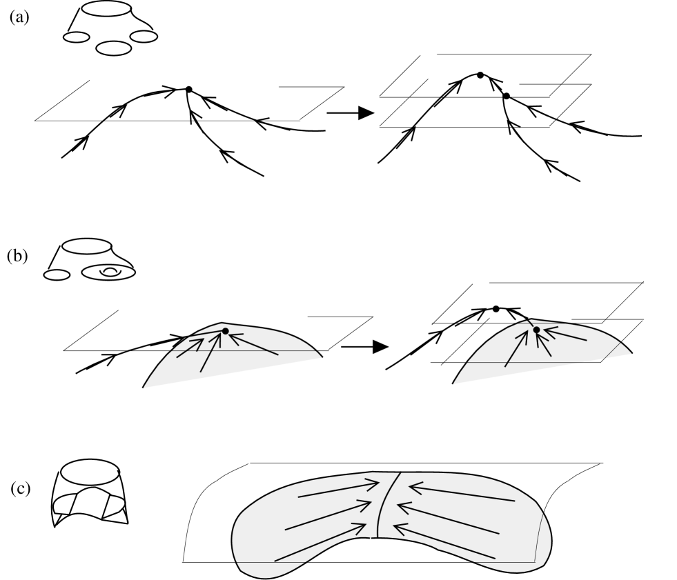
FIG. 4.: (a) and (b) are the example of the branching SOEP in an accidental timeslicing. They are understood by the small deformation of the timeslicing. On the other hand, (c) is the case in which the timeslicing is partially tangent to the SOEP. The two-dimensional SOEP behaves as the one-dimensional SOEP.

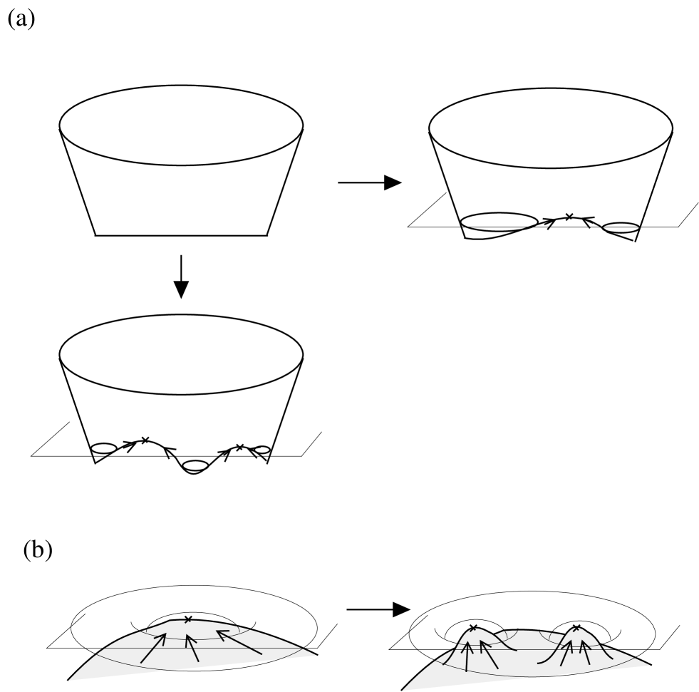
FIG. 5.: By the appropriate change of the timeslicing, the number of zeros of the vector field $\overline{K}$ changes. (a) and (b) are the one-dimensional and two-dimensional SOEP, respectively.

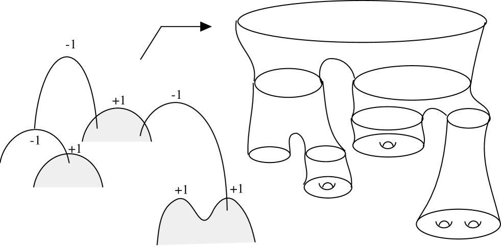
FIG. 6.: An example of the graph of the SOEP is drawn. Determining the order of the vertices, we see the TOEH from the index of each zero.

REFERENCES

- [1] S. W. Hawking and G. F. R. Ellice, The large scale structure of space-time Cambridge University Press, New York, 1973.
- [2] S. W. Hawking, Commun. Math. Phys. 25 (1972)152.
- [3] P. T. Chrusciel and R. M. Wald, Class. Quant. Grav. 11(1994)L147.
- [4] D. Gannon,Gen. Relativ. Gravit. 7 (1976)219.
- [5] J. L. Friedmann, K. Schleich and D. M. Witt, Phys. Rev. Lett. 71 (1993)1486.
- [6] T. Jacobson and S. Venkataramani, Class. Quantum Grav. 12 (1995)1055.
- [7] S. Browdy and G. J. Galloway, J. Math. Phys. 36 (1995)4952.
- [8] S. A. Hughes, C. R. Keeton, P. Walker, K. Walsh, S. L. Shapiro and S. A. Teukolsky, Phys. Rev. D49 (1994)4004, A. M. Abrahams, G. B. Cook, S. L. Shapiro and S. A. Teukolsky Phys. Rev. D49 (1994)5153, S. L. Shapiro, S. A. Teukolsky and J. Winicour Phys. Rev. D52 (1995)6982.
- [9] P. Anninos, D. Bernstein, S, Brandt, J. Libson, J. Massó, E. Seidel, L. Smarr, W. Suen, and P. WalkerPhys. Rev. Lett. 74 (1995)630.
- [10] R. M. Wald, General Relativity University of Chicago Press, Chicago, 1984.
- [11] R. D. Sorkin, Phys. Rev. D33 (1985)978.
- [12] R. P. Geroch, J. Math. Phys. 8 (1967)782.
- [13] P. T. Chruściel, G. J. Galloway, gr-qc/9611032.
- [14] I. M. Singer and J. A. Thorpe, Lecture Notes on Elementary Topology and Geometry Springer Verlag, 1976.
- [15] in preparation
- [16] S. Chandrasekhar, The mathematical theory of black holes, Oxford University Press Inc., New York, 1983.
- [17] S. W. Hawking,Comm. Math. Phys. 43 (1975)199.