The mixmaster universe: A chaotic Farey tale

Abstract

When gravitational fields are at their strongest, the evolution of spacetime is thought to be highly erratic. Over the past decade debate has raged over whether this evolution can be classified as chaotic. The debate has centered on the homogeneous but anisotropic mixmaster universe. A definite resolution has been lacking as the techniques used to study the mixmaster dynamics yield observer dependent answers. Here we resolve the conflict by using observer independent, fractal methods. We prove the mixmaster universe is chaotic by exposing the fractal strange repellor that characterizes the dynamics. The repellor is laid bare in both the 6-dimensional minisuperspace of the full Einstein equations, and in a 2-dimensional discretisation of the dynamics. The chaos is encoded in a special set of numbers that form the irrational Farey tree. We quantify the chaos by calculating the strange repellor’s Lyapunov dimension, topological entropy and multifractal dimensions. As all of these quantities are coordinate, or gauge independent, there is no longer any ambiguity–the mixmaster universe is indeed chaotic.

Einstein’s theory describes gravity from falling apples to the collapse of an entire universe. When space is most strongly deformed, Einstein’s nonlinear theory may be fundamentally chaotic. Chaotic systems are complex but knowable. A paradigm shift from simplicity to complexity is needed. The attempt to track each individual universe is abandoned. Instead, as with thermodynamics, the emergent properties of the collective are considered. Just as it is possible to understand a thermal collection of atoms from scant features, such as the temperature or the entropy, so too can chaotic cosmologies be understood from a fractal dimension or a topological entropy.

The singular cores of collapsing stars and the big bang are suspected to tend toward chaos [1, 2]. Beyond conjecture, attempts to conclusively identify chaos near singularities stirred debate[5, 6]. The debate has centered on the mixmaster universe, an archetypal singularity. In the mixmaster model, the three spatial dimensions oscillate anisotropically out of the big bang and finally toward a big crunch[7].

Relativistic chaos has the unique difficulty of demanding observer independent signatures. Many of the standard chaotic indicators such as the Lyapunov exponents and associated entropies are observer dependent. The Lyapunov exponent quantifies how quickly predictability is lost as a system evolves. The metric entropy quantifies the creation of information as time moves forward. They are both tied to the rate at which a given observer’s clock ticks. The relativism of space and time rejects the notion of a prefered time direction. In a curved space, the Lyapunov exponent and metric entropy become relative as well. Observer independent tools are needed to handle chaos in relativity.

The challenge of relativistic chaos is well demonstrated in the debate over the chaoticity of the mixmaster universe. Barrow studied the chaotic properties of a discrete approximation to the full dynamics known as the Gauss map [8, 9]. Belinski, Khalatnikov and Lifshitz developed the Gauss map which evolves the universe toward the singularity from bounce to bounce of the axes [2]. Barrow found the Lyapunov exponent, the metric entropy and topological entropy of the map. The dispute began when numerical experiments run in different coordinate systems found the Lyapunov exponents vanished [10, 11, 12, 13, 14]. Furthermore, the Gauss map itself corresponds to a specific time slicing. The ambiguity of time was manifest.

To conclude that the mixmaster approach to a singularity is indeed chaotic, an observer independent signature must be uncovered. As has been promoted elsewhere [15, 16, 17], fractals in phase space are observer independent chaotic signatures. Their existence and properties do not depend on the tick of a clock or the worldline of an observer. As well, fractals have an aesthetic appeal. The chaos is consequent of a lack of symmetries. The loss of symmetry in the dynamics is appeased by the emergent symmetry of the self-affine fractal[18] in phase space.

We exploit the observer independence of the fractal to show unambiguously that the mixmaster universe is chaotic. This result was announced in Ref. [17].

Fractals in the minisuperspace phase space of the full dynamics are uncovered. Probing the full dynamics is always numerically intensive. To open a window on the numerical results we also study the Farey map, a discrete approximation to the dynamics related to the Gauss map. We focus on the map analytically but the real power of the conclusions is in the full dynamics where no approximation is made. Just as with a geographical map, the Farey map is used as a guide to navigate through the full dynamical problem. We use the map to locate the skeleton of the chaos and then verify its existence with the numerics.

The bare bones of the chaos is revealed in an invariant subset of self-similar universes known collectively as a strange repellor. The strange repellor[20] is a fractal, nonattracting, invariant set (§II). More familiar are fractal, attracting, invariant sets or strange attractors. Though the repellor is a tiny subset of all possible universes, it isolates the essential features of the system[21]. A typical universe will accumulate chaotic transient eras as it brushes past the strange repellor in phase space.

The repellor is multifractal as shown in §II A. The Farey map divides the fractal into two complementary sets. A particularly elegant quality of the Farey map is the connection between these complementary sets and number theory. As elaborated in §II B, the multifractal can be completely understood in terms of continued fraction expansions and Farey trees.

In addition to the usual multifractal dimensions, we stress the importance of the Lyapunov dimension (§III A). This dimension is built out of a coordinate invariant combination of the Lyapunov exponent (§III C) and the metric entropy. Both the Lyapunov exponent and the metric entropy can then be reinstated as valid tools even in curved space. We introduce a method for handling the repellor as a Hamiltonian exit system, to facilitate calculation of the Lyapunov dimension (§III B).

Maps have been put to good use before. We devote §IV to a detailed comparison of the Gauss map and the Farey map. There are two main differences we draw out. One distinction is in the character of the maps themselves. They are not topologically equivalent and therefore have different topological features such as topological entropy. The other notable difference is the technique for handling the maps. Previous methods treat the set of all universes. We concentrate on the repellor subset. The previous techniques and ours are complementary.

Having isolated the repellor in the map, we use this insight as an x-ray to expose the chaotic skeleton in the full, unapproximated dynamics (§V).

I The Mixmaster Dynamics

The richness of Einstein’s theory is revealed in the spectrum of solutions to the dynamical equations. To solve these equations universe by universe, symmetries of the Hamiltonian are sought. The entire universe must necessarily have a conserved Hamiltonian. Energy cannot leak into or out of spacetime. Since the Hamiltonian effects translations in time, symmetries of the Hamiltonian lead to invariants or integrals of the motion and hence solutions to the equations of motion. However, strong gravity is nonlinearly entangled and we cannot expect the universe to typically offer up symmetries of the motion. Einstein’s equations are more likely than not to be fundamentally nonintegrable, and so chaotic.

The singularity structure of the equations can indicate if the system is integrable. It has been shown that the mixmaster equations fail the Painlevé test [22]. This suggests, but does not prove, that the system is nonintegrable.

The fractals we find in the minisuperspace phase space show conclusively the emergence of chaos. To begin, we use dynamical systems theory on sets of universes and consider the minisuperspace of all possible mixmaster cosmologies. The minisuperspace Hamiltonian is

$$H = (\ln{a})^{\prime}(\ln{b})^{\prime}+(\ln{a})^{\prime}(\ln{c})^{\prime}+(\ln{b})^{\prime}(\ln{c})^{\prime}$$ (1)

$$+ {1\over 4}\left[a^{4}+b^{4}+c^{4}-2(b^{2}c^{2}+a^{2}c^{2}+b^{2}a^{2})\right]$$ (2)

where $a,b,c$ are the scale factors for the three spatial axes. For a full description of the geometry see Refs. [7, 23]. The Hamiltonian constraint equation requires $H=0$. The equations of motion governing the behaviour of the three spatial axes are

$$(\ln a)^{\prime\prime}={1\over 2}\left[(b^{2}-c^{2})^{2}-a^{4}\right]\quad{\it et\;cyc.}\;(a,b,c)\;.$$ (3)

A prime denotes $d/d\tau$ where $\tau$ is related to the cosmic time $t$ through $dt=abc\,d\tau$. The universe comes out of the big bang with two axes oscillating between expansion and collapse while the third grows monotonically. The overall volume of the universe expands to a maximum and then collapses. On approach to the big crunch, two spatial dimensions will oscillate in expansion and collapse while the third will decrease monotonically. Eventually a bounce occurs at which point the axes permute and interchange roles.

The scale and expansion factors can be reparameterized in terms of the four variables $(u,v,\omega,\Omega)$[9]. As was done in reference [9], the initial conditions can be fixed on the surface of section $a_{o}=1$, $(\ln a)^{\prime}_{o}\geq 0$, without loss of generality

$$\ln{a_{o}}=0\,,\hskip 72.26999pt(\ln{a})_{o}^{\prime}={3(1+u_{o})\omega_{o}\over(1+u_{o}+u_{o}^{2})}\,,$$ (4)

$$\ln{b_{o}}={3\Omega_{o}\over(1+v_{o}+u_{o}v_{o})}\,,\quad(\ln{b})_{o}^{\prime}={-3\omega_{o}u_{o}\over(1+u_{o}+u_{o}^{2})}\,,$$ (5)

$$\ln{c_{o}}={3(v_{o}+u_{o}v_{o})\Omega_{o}\over(1+v_{o}+u_{o}v_{o})}\,,\quad(\ln{c})_{o}^{\prime}={3(u_{o}+u_{o}^{2})\omega_{o}\over(1+u_{o}+u_{o}^{2})}\,.$$ (6)

The relative sizes and velocities of the axes respectively are accounted for by $v$ and $u$. The overall scale factors $\Omega=(\ln(abc))/3$ and $\omega=\Omega^{\prime}$ grow monotonically away from the big bang to the maximum of expansion and then shrink monotonically toward the big crunch.

The evolution of a given universe can be viewed as a particle scattering off a potential in minisuperspace. The right hand side of Eqns. (3) play the role of a potential. When this potential is negligible, the evolution mimics a simple Kasner model. The Kasner metric is

$$ds^{2}=-dt^{2}+t^{2p_{a}}dx^{2}+t^{2p_{b}}dy^{2}+t^{2p_{c}}dz^{2}\ \ .$$ (7)

The Kasner indices can be parameterized as

$$p_{a}(u)={1+u\over(1+u+u^{2})},$$ (8)

$$p_{b}(u)={-u\over(1+u+u^{2})},$$ (9)

$$p_{c}(u)={u+u^{2}\over(1+u+u^{2})}\,,$$ (10)

and satisfy $\sum_{i=1}^{3}p_{i}=1=\sum_{i=1}^{3}p_{i}^{2}$. Moreover, $p_{a}(1/u)=p_{c}(u)$, $p_{b}(1/u)=p_{b}(u)$ and $p_{c}(1/u)=p_{a}(u)$. As is customary, we take $u$ to lie in the range $[1,\infty]$ to ensure a definite ordering of the Kasner exponents:

$$p_{b}<p_{a}<p_{c}\,.$$ (11)

In terms of conformal time,

$$(\ln a)^{\prime}\simeq p_{a}\quad\quad{\Longrightarrow}\quad\quad a\propto\exp(p_{a}\tau)\,.$$ (12)

When the potential gains importance, the trajectory is scattered and enters another Kasner phase. To study the effect of scattering it is a good approximation to consider only the change on the Kasner indices of Eqn. (10). The full dynamical problem can therefore be reduced to a map which evolves the parameter $u$ forward in discrete intervals of time. Belinski, Khalatnikov, and Lifshitz (BKL) reduced the dynamics to the $1$-dimensional Gauss map. The Gauss map evolves $u$ from bounce to bounce as the trajectory strikes the potential. We focus instead on a $2$-dimensional map, the Farey map, which includes not only bounces but also oscillations [2, 9, 24, 25]. The Farey map has the additional property of being invertible and so preserves the time reversibility of Einstein’s equations [26].

II The Farey map and the strange repellor

With the discrete time map we are able to isolate the repellor. The repellor is the chaotic subset of self-similar universes. It is the Hamiltonian analogue of the better known strange attractor. In dissipative systems, the volume of phase space shrinks and trajectories are drawn onto an attracting set as energy is lost. Since the universe is a self-contained Hamiltonian system, there can be no dissipation and so no attractors. Still, the notion of an invariant set can be an incisive characterization of the system.

Nonattracting invariant sets are referred to as repellors since all trajectories which constitute the set are unstable in at least one eigendirection, and in that sense repel any near neighbours. The phase space volume is conserved as it squeezes in one direction while it expands in the other as it careens off the repellor. The transient chaos experienced by a typical, aperiodic universe reflects the passage of that trajectory near the core periodic orbits.

Khalatnikov and Lifshitz[1] were the first to introduce the $u$ parameterisation and derive the evolution rules:

$$u\rightarrow u-1\quad{\rm if}\quad u>1$$ (13)

$$u\rightarrow 1/u\quad{\rm if}\quad u<1\,.$$ (14)

As it stands, this prescription is discontinuous at $u=1$. A continuous map can derived by considering either of the two double transformations

$$u^{\prime}=u-1\quad{\rm and} \quad u^{\prime\prime}=1/u^{\prime}\quad{\rm or}$$ (15)

$$u^{\prime}=1/u\quad{\rm and} \quad u^{\prime\prime}=u^{\prime}-1\,.$$ (16)

This leads to the two entirely equivalent continuous maps

$$u_{n+1}=\left\{\begin{array}[]{ll}u_{n}-1,&u\geq 2\\ {\displaystyle{1\over u_{n}-1}},&1\leq u<2\end{array}\right.\,,$$ (17)

and

$$u_{n+1}=\left\{\begin{array}[]{ll}u_{n}-1,&u\geq 1\\ {\displaystyle{1\over u_{n}}-1},&0\leq u<1\end{array}\right.\,.$$ (18)

Both choices have shown up in the literature over the years, but these days the first choice is prefered as the transitional step where $u<1$ is hidden in the double transformation. By hiding this step, a definite Kasner ordering can be maintained. It is worth mentioning that the two maps use exactly the same $u$ variable, even though the first can be formally be recovered from the second by making the substitution $u=\tilde{u}-1$.

By combining the $u$-map with its inverse in terms of $v$, one arrives at the two dimensional Farey map. We call the map a Farey map due to its connection to the Farey trees of number theory as discussed in §II A. The Farey map evolves the two parameters forward by discrete intervals in time, $F(u_{n},v_{n})=(u_{n+1},v_{n+1})$, according to the rule

$$F(u,v)=\left\{\begin{array}[]{lll}u-1,&\ v+1\,,&u\geq 1\quad({\rm oscillations})\\ &&\\ {\displaystyle{1\over u-1}},&{\displaystyle{1\over v}+1}\,,&u<1\quad{\rm(bounces)}\end{array}\right.$$ (19)

The map describes the evolution of a universe through a series of Kasner epochs. If $u\geq 2$, then two axes oscillate in expansion and collapse while the third coasts. The axes will oscillate until $u<2$ at which point a bounce occurs, the three axes interchange roles, and $u$ is bounced about the numberline. In some studies, what we call oscillations are called epochs and what we call bounces are called eras.

Running in parallel with the Farey map is the Volume map $V(\Omega,\omega)$ described by

$$\Omega_{n+1}=\Omega_{n}\left[1+{1+u_{n}+u_{n}^{2}\over u_{n}(1+v_{n}+u_{n}v_{n})}\right]\,,$$ (20)

(21)

$$\omega_{n+1}=\omega_{n}\left[1-{2u_{n}\over 1+u_{n}+u_{n}^{2}}\right]\,.$$ (22)

Like the Farey map, the Volume map is a good approximation to the exact evolution away from the maximum of expansion where $\omega$ flips sign. During the collapse phase $\tau\rightarrow-\infty$, $\omega>0$ and $\Omega<0$. A nice feature of the combined Farey-Volume map, $M(u,v,\Omega,\omega)$, is the way it splits the dynamics into oscillatory and monotonic pieces.

Clearly, the monotonic behaviour of the $V$-map excludes the possibility of periodic trajectories for the $M$-map. Since all chaotic behaviour relies on the existence of unstable periodic trajectories, this would seem to rule out chaos in the mixmaster dynamics. Indeed, similar reasoning has been used to claim that the full mixmaster equations cannot be chaotic[27]. The flaw in this reasoning was to neglect the non-compact nature of the mixmaster phase space. For example, the non-compact motion along a spiral of fixed radius appears as circular motion in an appropriate comoving frame of reference. Although a spiral trajectory never returns to its starting point, the motion is periodic in a projected subset of phase space. Similarly, the mixmaster dynamics allows unstable periodic trajectories in terms of the $(u,v)$ coordinates. A projected strange repellor is all we require for chaos to occur. Consequently, we can drop the overall scaling of the $V$-map and concentrate on the Farey map. Similarly, when we turn our attention to the full dynamics we will look for periodic behaviour in scale invariant quantities such as $(\ln b)/(\ln c)$. In this way we effectively project out the regular evolution of the system.

A universe initiated with some condition $(u_{o},v_{o})$ will evolve through a series of oscillations and bounces as prescribed by the map. For a typical universe, $u$ and $v$ will randomly be tossed about the numberline. An important subset of universes are formed by the orbits periodic in $(u,v)$. The existence of a repelling, denumerably infinite, everywhere dense set of periodic orbits was first recognised by Bogoyavlenski and Novikov[28]. Physically, the periodic orbits correspond to discretely self-similar universes. After one orbital period, the proportionality of the scale and expansion factors recur, while the volume of the universe has contracted overall. These collection of periodic orbits in $(u,v)$ form a multifractal strange repellor.

To isolate the strange repellor we search for a chaotic, nonattracting, invariant set. In this section we justify each term in this definition.

Invariant set: The set of points which are invariant in time are located by the condition

$$F^{k}(\bar{u}_{i},\bar{v}_{i})=(\bar{u}_{i},\bar{v}_{i})$$ (23)

for $k=1,\dots,\infty$. These fixed points lie on periodic orbits of period $p\leq k$. Iteration of the map $k$-times, just returns a point on a period $k$ orbit to itself. For Hamiltonian systems it is sufficient to consider the future invariant set as time reversal invariance can be used to find the complete strange repellor. For the Farey map the future invariant set is defined by the condition

$$F^{k}(\bar{u}_{i})=\bar{u}_{i}\,,\quad(v\;{\rm arbitrary}).$$ (24)

Consider for illustration the period 1 orbit. The invariant point satisfies $F(\bar{u}_{1})=\bar{u}_{1}$. The map can be split into an oscillation map $O$ and a bounce map $B$;

$$O(u_{n}) = u_{n}-1\quad\quad u_{n}\geq 2$$ (25)

$$B(u_{n}) = {1\over u_{n}-1}\quad\quad u_{n}<2\ \ .$$ (26)

The equation $F(\bar{u}_{1})=\bar{u}_{1}$ yields two possibilities: $O(\bar{u}_{1})=\bar{u}_{1}$ or $B(\bar{u}_{1})=\bar{u}_{1}$. Only the bounce fixed point, which generates the equation

$$\bar{u}_{1}={1\over\bar{u}_{1}-1}\ \ ,$$ (27)

has a solution. The solution is the golden mean

$$\bar{u}_{1}={\sqrt{5}+1\over 2}\ \ .$$ (28)

The occurrence of the golden mean is no accident. As we discuss in the next section, it is the first leaf on the irrational Farey tree. No matter how far into the future we try to evolve this initial condition, we get $\bar{u}_{1}$ back. A universe initiated with axes and velocities parameterized by $\bar{u}_{1}$ will scale in a self-similar manner as $u$ is returned to $\bar{u}_{1}$ with each jump forward in time.

Another particularly simple set of fixed points can be located. These are the maximal value of $u$ along a period $k$ orbit. The maximal value of $u$ corresponds to the largest number of oscillations before a bounce. The equation $O^{k-1}B(\bar{u})=\bar{u}$ generates

$$\bar{u}_{k}(\bar{u}_{k}-k)=1\,,$$ (29)

whose solution is

$$\bar{u}_{k}={k+\sqrt{k^{2}+4}\over 2}\ \ .$$ (30)

These are the silver means (and can be found among the $k$th order leaves in the Farey tree). As elaborated in the next section, all of the fixed points comprise a countably infinite set of irrationals with periodic continued fraction expansions described by Farey trees. In this sense, we know all the fixed points.

Nonattracting: We can verify that all of the periodic orbits are unstable and so are not attracting but rather repelling. The repellor is the intersection in phase space of the unstable and stable manifolds. Since it is unstable in one direction, a near neighbour to a periodic orbit will deviate off the invariant set. Conservation of the Hamiltonian requires the other eigendirection be attracting.

In the 2-D phase space defined by $(u,v)$, we show here that the unstable manifold is composed of fixed points along $u$. This is the future invariant set given by Eqn. (24). Since time reversal corresponds to $(u,v)\rightarrow(v,u)$, the stable manifold is made up of the fixed points along $v$. The stable and unstable manifolds intersect at each point along a periodic orbit. The collection of such points form the strange repellor. Since they are invariant, any point which is on both the unstable and stable manifolds will be mapped to points which by necessity inhabit at the intersection of stable and unstable manifolds.

To demonstrate explicitly that the periodic orbits are unstable in the $u$ direction but attracting in $v$ consider an initial trajectory in the vicinity of a period $p$ orbit. We look at the evolution in the $u$ direction first. The aperiodic universe begins with $u_{o}=\bar{u}_{o}+\delta_{o}$ where $\bar{u}_{o}$ is the fixed point along the periodic universe. A period later, the deviation from the periodic orbit has grown to $\delta_{p}$ defined by [29]

$$F^{p}(u_{o})=u_{o}+\delta_{p}=F^{p}(\bar{u}_{o}+\delta_{o})\ \ .$$ (31)

Expanding the right hand side we can relate the evolved deviation to the initial deviation

$$\delta_{p}=c_{p}\delta_{o}$$ (32)

where the stability coefficient is

$$c_{p} \equiv \left.{dF^{p}(u_{n})\over du_{n}}\right|_{u_{n}=\bar{u}_{o}}$$ (33)

$$= F^{\prime}(\bar{u}_{o})F^{\prime}(\bar{u}_{1})...F^{\prime}(\bar{u}_{p-1})\ \ .$$ (34)

The elements in the final product are evaluated at the points along the unperturbed orbit. The periodic orbits are stable if the magnitude of $\delta_{p}$ shrinks and unstable if the magnitude grows. In terms of the stability coefficient the periodic orbits are stable if $|c_{p}|<1$ and unstable if $|c_{p}|>1$. Taking the derivative of the map

$$\left|F(u,v)^{\prime}\right|=\left\{\begin{array}[]{lll}1,&\quad 1&\quad(u\geq 2)\\ &&\\ {\displaystyle{1\over(u-1)^{2}}},&{\displaystyle{1\over v^{2}}}&\quad(u<2)\end{array}\right.\ \ .$$ (35)

Along any periodic orbit, at least one point must fall between 1 and 2. Let $\bar{u}_{{\rm min}}$ be the smallest value of $\bar{u}$ along the orbit. It then follows from (33) that

$$\left|c_{p}\right|\geq(\bar{u}_{{\rm min}}-1)^{-2}>1\,.$$ (36)

Therefore all orbits on the repellor are unstable in the $u$ eigendirection. Any universe which begins near an exact periodic orbit eventually deviates away from that orbit in $u$ and is not attracted onto it. Since a typical universe is confined to bounce around the numberline forever it will eventually scathe past a periodic orbit before being repelled off only to accidentally stumble onto the repellor again. Thus, a typical universe will scatter around intermittently hitting chaotic episodes as it jumps on and off the repellor.

Repeating the stability analysis in $v$, we find $|c^{v}_{k}|=1/v^{2}<1$. Near neighbours tend to follow periodic orbits in the $v$ direction. The repellor along $u$ is an attractor along $v$.

Chaotic: We have so far established that the periodic orbits comprise a nonattracting, invariant set. We can demonstrate that this set is chaotic by showing it has a positive topological entropy. The topological entropy, in analogy with the thermodynamic entropy, measures the number of accessible states on the repellor. The number of states on the repellor is equivalent to the number of fixed points so

$$H_{T}=\lim_{k\rightarrow\infty}{1\over k}\ln N(k)$$ (37)

where $N(k)$ is the number of fixed points. For a nonchaotic set, the number of fixed points is either finite or grows as a finite power of $k$, so $H_{T}=0$.

The fixed points at order $k$ are found by solving equation (24): $F^{k}(\bar{u}_{i})=\bar{u}_{i}$. To count the number of fixed points we can count the number of such possible equations. For a given period $p\leq k$, $F^{k}$ can be broken into $O^{m}$ oscillations and $B^{k-m}$ bounces. Since $O$ and $B$ do not commute, the order in which they occur leads to different possible solutions for the $\bar{u}_{i}$. The number of ways to combine $m$ $O$’s and $k-m$ $B$’s is

$$\pmatrix{k\cr m}={m!\over m!(k-m)!}$$ (38)

For example, after $k=4$ iterations of the map and $m=2$ oscillations and $k-m=2$ bounces there are $6$ possible permutations:

$$OOBB(\bar{u}_{i}) = \bar{u}_{i}$$ (39)

$$BBOO(\bar{u}_{i}) = \bar{u}_{i}$$ (40)

$$BOOB(\bar{u}_{i}) = \bar{u}_{i}$$ (41)

$$OBBO(\bar{u}_{i}) = \bar{u}_{i}$$ (42)

$$OBOB(\bar{u}_{i}) = \bar{u}_{i}$$ (43)

$$BOBO(\bar{u}_{i}) = \bar{u}_{i}$$ (44)

However, the first $4$ are all cyclic permutations of $OOBB$. Cyclic permutations must lie along the same orbit. Therefore, the solutions to the first $4$ equations yield the points along the same period $4$ orbit. Similarly, the last $2$ are cyclic permutations of each other. They represent the recurrence of the two points along the period $2$ orbit.

The total number of points belonging to the future invariant set with period $p\leq k$ is given by summing over all possible combinations of oscillations and bounces:

$$N(k)=\sum_{m=0}^{k-1}\pmatrix{k\cr k-m}=2^{k}-1\ \ .$$ (45)

There are thus $2^{k}-1$ words of length $k$ that can be built out of a $2$ letter alphabet. The topological entropy is then

$$H^{u}_{T}=\ln 2\ \ .$$ (46)

This entropy is independent of phase space coordinates. The topological entropy for the full 2-D map $F(u,v)$ will be twice this quantity as the strange repellor is formed by the intersection of $2^{k}-1$ horizontal and vertical lines. Thus, there are $(2^{k}-1)^{2}$ roots of Eqn.(23) at order $k$ and $H_{T}=2\ln 2$. The result $H^{u}_{T}=\ln 2$ was first found by Rugh[10] using symbolic dynamics to describe typical, aperiodic orbits in $u$.

The topological entropy will be the same for all maps which are topologically conjugate; that is, which can be related by a continuous, invertible, but not necessarily differentiable, transformation of coordinates. In particular, this tells us that the map $F(u)$ can be obtained from the shift map, horseshoe map or generalised baker’s map[29]. We mention that the closely related Gauss map has a much higher topological entropy $H_{T}={\pi^{2}/(6\ln 2)}$. As discussed in §IV, the two maps are not topologically conjugate. We do not expect then for their entropies to be the same.

The bare bones of the chaotic scattering has been exposed in the repellor. Taking this skeleton, we can now show that the repellor is in fact strange, that is, fractal.

A The Repellor is a Multifractal

We can create an illustrative picture of the fractal set of self-similar universes. Distributing the fixed points $u$ along the numberline, the collection of periodic points form a fractal in phase space. A fractal is a nowhere differentiable, self-affine structure. It cannot be undone by a coordinate transformation. The emergence of a fractal distribution of invariant points is an observer independent declaration of chaos.

For multifractals there is information in the way points are distributed. There is an underlying fractal structure with an architecture of distributed points built on top. The fractal in phase space is simply constructed by locating all of the points along period $p\leq k$ orbits numerically and plotting them in a histogram as is done in Fig. 1. The histogram was generated by solving for all roots of Eqn. (24) up to and including $k=16$. The histogram reveals how points are distributed in the future invariant set, otherwise known as the unstable manifold of the strange repellor. The self-similarity of the distribution is clear.

The distribution of points can be understood in terms of the period of the orbit. As $k$ increases, the lowest period orbit, namely the $p=1$ orbit, is visited the maximal number of times, that is, $k$ times. On the other hand, the maximum value of $u$ at order $k$ lies on a $p=k$ orbit, and so is visited only once.

Points on the repellor are clustered in the interval $1<u<2$. The combinatorics of building words out of a $2$-letter alphabet $(O,B)$ of oscillations and bounces favours the small $u$ tower. Consider the integer interval $[n,n+1]$. A root in this interval corresponds to the sequence, or word, $O^{(n-1)}B$ occuring somewhere along the orbit. The complete orbit is a sentence of $O^{i}B$ words, eg. $(O^{2}B)(B)(O^{5}B)(OB)$, repeated in a cyclic fashion. Since the number of $n$-letter words that can be formed from a 2-letter alphabet is $2^{n}$, it follows that the fraction of roots in each interval is

$$\rho_{n}=2^{-n}.$$ (47)

Note that the distribution is correctly normalised since

$$\sum_{n=1}^{\infty}\rho_{n}=1\,.$$ (48)

The exponential fall off in the density of points on the repellor is clearly evident in Fig. 1.

The parameterization of the axes in terms of $u$ in Eqn. (8) shows that the small $u$ orbits typical of the repellor are those with axes of similar scale and speed. These universes have axes which frequently switch from expansion to collapse. It follows that the strange repellor corresponds to the most isotropic mixmaster trajectories possible.

In the full 2-D phase space of the Farey map, $F(u,v)$, the unstable manifold appears as a forest of vertical lines, while the stable manifold appears as a forest of horizontal lines. A portion of the future invariant set, the unstable manifold of the repellor, is displayed in Fig. 2. The collection of lines appear to form a multifractal cantor set. To confirm this, we calculate the fractal dimension of the set.

The fractal dimension can be thought of as a critical exponent. The dimension is a measure of the length of the collection of points. To find its box-counting dimension, cover the set with $N(\epsilon)$ boxes of size $\epsilon$. As the size of the boxes is taken infinitesimally small, the number of boxes needed to cover the set grows. For fractals, the number of boxes needed grows faster than the scale shrinks. The structure becomes more and more complex as smaller and smaller scales come into focus. The critical exponent can be defined as the number which keeps

$$\lim_{\epsilon\rightarrow 0}\epsilon^{D_{o}}N(\epsilon)$$ (49)

finite. Any exponent greater than $D_{o}$ would result in zero length, and an exponent smaller would result in infinite length. In this sense $D_{o}$ is a critical exponent.

This dimension can be generalized to include not just the scaling property of the fractal but also the distribution of points on top of the underlying foundation. This leads to a continuous spectrum of critical exponents or dimensions. The spectrum of dimensions is more commonly expressed as

$$D_{q}={1\over q-1}\lim_{\epsilon\rightarrow 0}{\ln\sum_{i=1}^{N(\epsilon)}(p_{i})^{q}\over\ln\epsilon}\;,$$ (50)

where $N(\epsilon)$ are the number of hypercubes of side length $\epsilon$ needed to cover the fractal and $p_{i}$ is the weight assigned to the $i^{{\rm th}}$ hypercube. The $p_{i}$’s satisfy $\sum_{i=1}^{N(\epsilon)}p_{i}=1$. The standard capacity dimension $D_{o}$ is recovered when $q=0$, the information dimension when $q=1$, the correlation dimension when $q=2$ etc. For homogeneous fractals all the various dimensions yield the same result. The multifractal dimensions $D_{q}$ are invariant under diffeomorphisms for all $q$, and $D_{1}$ is additionally invariant under coordinate transformations that are non-invertible at a finite number of points[30].

The quantitative importance of the fractal dimension is expressed in terms of the final state sensitivity $f(\delta)$[31]. This quantity describes how the unavoidable uncertainty in specifying initial conditions gets amplified in chaotic systems, leading to a large final state uncertainty. By identifying a number of possible outcomes for a dynamical system, the space of initial conditions can be divided into regions corresponding to their outcome. If the system is chaotic, the boundaries between these outcome basins will be fractal. Points belonging to the basin boundary are none other than the chaotic future invariant set. The function $f(\delta)$ is the fraction of phase space volume which has an uncertain outcome due to the initial conditions being uncertain within a hypersphere of radius $\delta$. It can be shown[31] that

$$f(\delta)\sim\delta^{\alpha}\;,\quad\alpha=D-D_{0}\;,$$ (51)

where $D$ is the phase space dimension and $D_{0}$ is the capacity dimension of the basin boundary. For non-chaotic systems $\alpha=1$ and there is no amplification of initial uncertainties, while for chaotic systems $0<\alpha<1$ and marked final state sensitivity can occur.

It can be argued that the capacity dimension must equal the phase space dimension for the mixmaster repellor. The periodic orbits are given by the periodic irrationals as explained in §II B. The periodic irrationals are dense on the numberline. Formally this means there is always another periodic irrational $\epsilon$ away from a neighbour for all $\epsilon>0$. Since the periodic orbits are dense, there will always be an infinite number of fixed points in any box. It is sufficient to cover the set then with $N(\epsilon)\sim 1/\epsilon^{2}$ boxes. Therefore, the basic box counting dimension is $D_{o}=D=2$ [32], though it converges slowly. In the infinite time limit this can be interpreted as an ultimate loss in predictability since $f(\delta)=1$. The mixmaster is very mixed.

While the box counting dimension saturates at the phase space dimension, the more heavily weighted dimensions of Eqn. (50) do not. Taking the information dimension of the fractal in Fig. 2, we find

$$D^{u}_{1}=1.87\pm 0.01\ \ .$$ (52)

Fig. 3 shows the fit used to determine $D^{u}_{1}$. The quality of the fit gives us confidence that the strange repellor is truly fractal.

By forming the intersection of the Farey map’s stable and unstable manifolds, ie. by solving Eqn. (23) for all fixed points $(\bar{u},\bar{v})$, we uncover the strange repellor. A portion of the strange repellor is shown in Fig. 4 using all roots up to $k=12$. While it is possible to find the information dimension of the strange repellor directly from Fig. 4, the effort can be spared. Since the Farey map is Hamiltonian, we know the stable and unstable manifolds of the strange repellor share the same fractal dimensions. That is, $D^{u}_{1}=D^{v}_{1}=1.87\pm 0.01$. Now, the repellor is formed from the intersection of the stable and unstable manifolds, so its information dimension is simply

$$D_{1}=D^{u}_{1}+D^{v}_{1}-D=1.74\pm 0.02\,.$$ (53)

Since $D_{o}\neq D_{1}$, we have confirmed the multifractal nature of the strange repellor. The dimension of Eqn. (53) is calculated with all fixed points occurring at order $k=16$. As $k$ increases this number will continue to grow slowly as the rarified regions of the fractal continue to be populated. Thus, (53) actually represents a lower bound. However, we expect the ultimate value should only differ in the second decimal place.

B Farey trees

The fractal of Fig. 4 reveals two complementary sets. The sequence of gaps correspond to the rational numbers. In a complementary fashion, the strange repellor is made up from the periodic irrationals. Both sets are of Lebesgue measure zero. This division of the numberline can be understood in terms of the properties of the continued fraction expansions (cfe). We can write any number, rational or irrational, in terms of a cfe. While the connection to cfe’s was known and explored by Belinskii, Khalatnikov and Lifshitz, they explicitly ignored the periodic irrationals [2]. We focus on the periodic irrationals as they constitute the strange repellor.

Consider some initial condition, $u_{o}$, not necessarily on a periodic orbit. We can decompose any number into its integer part and some left over:

$$u_{o}=m_{o}+x_{o}\,,$$ (54)

where $m_{o}=[u_{o}]$ denotes the integer part of $u_{o}$ and $x_{o}$ the fractional excess. According to the map, the next value of $u$ following a bounce is $u_{1}=1/x_{o}$. Now decompose $1/x_{o}=m_{1}+x_{1}$, so that $m_{1}\geq 1$. Solving this for $x_{o}$ we find $x_{o}=1/(m_{1}+x_{1})$. At the next bounce $u_{2}=1/x_{1}$ so that $x_{1}=1/(m_{2}+x_{2})$. In this way we generate the cfe for $u_{o}$

$$u_{o}=m_{o}+{1\over{m_{1}+{\displaystyle{1\over m_{2}{\displaystyle+{1\over...}}}}}}\ \ ,$$ (55)

where $m_{i}\geq 1$ $\forall i$. The integers $m_{i}-1$ represent the number of oscillations between bounces. In shorthand form the cfe can be written as $u_{o}=[m_{0},m_{1},m_{2},m_{3},m_{4},\dots]$.

The map naturally distinguishes numbers on the basis of their cfe. A rational number can be written as the ratio of integers $x_{o}=p/q$. Consequently, the cfe is finite. The fact that its finite means at some iteration $u_{n+1}=\infty$ and rationals are tossed out of the map. At the opposite extreme, the periodic orbits on the repellor have infinite cfe’s which repeat. For example, an orbit of the form $\{O^{i-1}BO^{j-1}B\}$, where the curly brackets denote a repeated pattern, has the expansion

$$u_{o}=i+{1\over{\displaystyle{j+{1\over{\displaystyle i+{1\over{\displaystyle j+{1\over{\displaystyle i+...}}}}}}}}}\ \ .$$ (56)

In shorthand form this reads $u_{o}=[\{i,j\}]$. Lagrange showed that the necessary and sufficient condition for an irrational number to have a periodic cfe is for it to be the root of a quadratic equation with integer coefficients. It is easy to prove that the Farey-map gives such equations for the periodic orbits at every order in $k$.

The map generates a Farey tree [33]. Consider the initial condition $\bar{u}_{o}=1$. With the first iteration of the map, ie. with the first attempt to evolve that universe forward in time, $u$ is thrown to infinity. After two iterations, a universe with the initial condition $\bar{u}_{o}=2$ will be thrown to infinity. At the $k$th application of the map, after the universe has evolved forward in $k$ jumps, another group of universes whose initial conditions were rational numbers are discarded. The pattern of discarded terms is a Farey tree [34]. Farey trees also arise in the quasiperiodic route to chaos described by the circle map [33].

In the interval $[1,2]$ the Farey tree can be written as

$$\underbrace{\left(\frac{1}{1}\right)}_{k=0},\;\underbrace{\left(\frac{2}{1}\right)}_{k=1},\;\underbrace{\left(\frac{3}{2}\right)}_{k=2},\;\underbrace{\left(\frac{4}{3},\frac{5}{3}\right)}_{k=3},\;\underbrace{\left(\frac{5}{4},\frac{7}{5},\frac{8}{5},\frac{7}{4}\right)}_{k=4},\;\dots$$ (57)

The bracketed terms each comprise a level of the Farey tree. For all $k\geq 2$, there are $2^{k-2}$ leaves at order $k$. Every rational number in the interval [1,2] occurs exactly once somewhere on the Farey tree. Each leaf on the Farey tree has a continued fraction expansion that satisfies

$$\sum_{i=1}m_{i}=k\,.$$ (58)

Now, we see that each $m_{i}$ corresponds to a $m_{i}$-letter word $O^{(m_{i}-1)}B$. Each rational number corresponds to a sentence of these words. For example, at level $k=5$ we have the Farey number $10/7=[1,2,3]$, which gives rise to the sentence $BOBOOB$. At the same order we also have $6/5=[1,5]=BOOOOB$, and $9/5=[1,1,4]=BBOOOB$ etc. In other words, a universe which began with $\bar{u}_{o}=10/7$ will follow the pattern of $BOBOOB$ and then gets tossed to infinity. The universe then evolves with two axes fixed and the third expanding as $\propto t$. Such a universe has the form of a Rindler wedge $\times R^{2}$ [35].

At the opposite extreme from the rationals which escape the map are the periodic subset of irrationals. This explains the occurrence of the golden mean as the period $1$ orbit with no oscillations. Its cfe is

$${\sqrt{5}+1\over 2}=1+{1\over{1+{\displaystyle{1\over{\displaystyle 1+...}}}}}=[\{1\}]\ \ .$$ (59)

Numbers with a periodic cfe are a set of measure zero among the irrationals, though they are dense on the numberline.

An irrational Farey tree for the repellor can be constructed using the rational Farey tree as a seed. Consider the construction in the interval $[1,2]$. For each leaf on the rational Farey tree given by $[1,m_{1},m_{2},\dots,m_{k}]$, add a leaf to the irrational tree given by $[1,\{m_{1},m_{2},\dots,m_{k}\}]$. There are $2$ times as many leaves on the irrational Farey tree than there are on the rational Farey tree. This follows since all rationals have two continued fraction expansions. The two cfe’s differ in how they end. In general

$$[m_{0},\dots,m_{j}+1]=[m_{0},\dots,m_{j},1]\,.$$ (60)

Consider $10/7=[1,2,3]$. We see that $10/7$ also equals $[1,2,2,1]$. Thus, $10/7\approx 1.429$ has two corresponding leaves on the irrational Farey tree, $(\sqrt{15}-1)/2\approx 1.436$ and $(\sqrt{85}+5)/10\approx 1.422$. Consequently each rational generates two nearby irrationals.

A number theory result tells us that

$$\left|\alpha_{\pm}-{p\over q}\right|<{1\over 2q^{2}}\leq{1\over 2k^{2}}\,,$$ (61)

where $\alpha_{\pm}$ stands for the two irrational numbers that lie on each side of their rational seed. As $k\rightarrow\infty$ the leaves on the rational and irrational Farey trees get closer and closer together. Another result from number theory tells us that $\alpha_{+}>p/q$ and $\alpha_{-}<p/q$ (hence the names). The $1/q^{2}$ gaps around the rational Farey numbers seen in Figs. 1& $\!2$ are a consequence of this number theory result.

The asymptotic distribution of roots goes as follows: At level $k$ there are $2^{k-2}$ leaves on the rational Farey tree in the interval [1,2]. Each leaf produces 2 leaves on the irrational Farey tree. Thus, there are $2^{k-1}$ roots in the interval $[1,2]$ at level $k$. This matches our earlier results that there are $\sim 2^{k}$ roots at order $k$, half of which lie in the interval $[1,2]$.

Our brief excursion into number theory has produced a neat picture: The rational Farey tree gives us all the numbers that get mapped to $u=\infty$, while the irrational Farey tree gives us all the periodic orbits. The leftovers are all the irrationals, save the rational and irrational Farey trees, both of which have measure zero. Thus, all typical trajectories are aperiodic, unbounded and of infinite length. These are the trajectories typically studied in the literature. Our study is complementary.

C Lyapunov Exponents

In flat space, the extreme sensitivity of the dynamics can be quantified by Lyapunov exponents and the related metric entropy. The Lyapunov exponents determine how quickly in time trajectories diverge. The metric entropy measures the rate at which information is created. Since the exponent and the entropy are rates, they connect directly with the rate at which time pushes forward. Clearly, the observer dependence of the rate at which clocks tick make these tools suspect in the hands of relativists. Relativists abandon such coordinate dependent indicators.

Although Lyapunov exponents are observer dependent and therefore ambiguous in general relativity, we see in §III A that they are related to an observer independent quantity; namely, the Lyapunov dimension. Since there is still utility in them, we take the time to compute some Lyapunov exponents.

Since we know all the periodic orbits of the Farey map analytically, we are in a position to calculate the Lyapunov exponents for trajectories belonging to the Farey repellor. As a warm up we calculate the Lyapunov exponents for the the golden and silver mean orbits. Then we use the irrational Farey tree to write an analytic expression for the Lyapunov exponent for any periodic orbit on the repellor.

In close analogy to the manner in which the stability coefficient was found, the Lyapunov exponent for a given orbit is defined by

$$\lambda=\lim_{T\rightarrow\infty}{1\over T}\sum_{n=0}^{T-1}\ln\left|F^{\prime}(u_{n})\right|$$ (62)

where the $u_{n}$ are the points along the orbit under scrutiny. The Lyapunov exponents along $v$ are the negative of those along $u$ as we now show. The points along a periodic orbit are the same whether time runs forward or backward. Time reversal corresponds to inverting the map. Note that $(F^{-1})^{\prime}(u)=1/F^{\prime}(u)$ and therefore $\ln|{F^{-1}}^{\prime}(u)|=-\ln|F^{\prime}(u)|$. Since $F^{-1}(u,v)=F(v,u)$ it follows that $\ln|F^{\prime}(v)|=-\ln|F^{\prime}(u)|$. This identity in eqn (62) shows that

$$\lambda^{v}=-\lambda^{u}\ \ ,$$ (63)

as must be the case to conserve the phase space volume in the Hamiltonian system.

In illustration consider the golden mean period 1 orbit. All the $\bar{u}_{n}=\bar{u}_{1}$ and

$$F^{\prime}(u_{n})=-(\bar{u}_{1}-1)^{-2}=-(\bar{u}_{1})^{2}\,.$$ (64)

From Eqn. (62) it follows that

$$\lambda_{1}=\lim_{T\rightarrow\infty}{1\over T}(T-1)\ln\bar{u}_{1}^{2}\,,$$ (65)

which reduces to

$$\lambda_{1}=2\ln{1+\sqrt{5}\over 2}\simeq 0.9624\ \ .$$ (66)

Similarly, for the silver means (30) we can find the exponent. We know the maximum value of $u$ along the silver orbit is given by $u_{{\rm max}}=(\sqrt{k^{2}+4}+k)/2$, so the sum of the $\ln$’s in Eqn. (62) becomes the $\ln$ of the product,

$$F^{\prime}(\bar{u}_{0})F^{\prime}(\bar{u}_{1})...F^{\prime}(\bar{u}_{k-1})=-(\bar{u}_{{\rm max}})^{-2}\ \ .$$ (67)

After $k$ applications of the map, $F^{k}(\bar{u})=\bar{u}$, so that after $T$ application, a given value of $\bar{u}_{n}$ has repeated $[T/k]=T/k$ times. Thus $T$ must be a multiple of $k$. The sum in the (62) can be written

$$\sum_{n=0}^{T-1}\ln\left|F^{\prime}(u_{n})\right|=\left[{T-1\over k}\right]2\ln{\bar{u}_{{\rm max}}}$$ (68)

Which gives

$$\lambda_{k}={2\over k}\ln{k+\sqrt{k^{2}+4}\over 2}\ \ .$$ (69)

We have found the Lyapunov exponents for the two extreme cases of the period $1$ orbit and the longest period $k$ orbit. We now use the irrational Farey tree to write down the general expression for Lyapunov exponents:

$$\lambda=2\left(\sum_{i=0}m_{i}\right)^{-1}\sum_{{\rm cyc}}\ln\left([\{m_{1};m_{2},\dots\}]\right)\,,$$ (70)

where the second sum is taken over all terms in the cycle $\{m_{1},m_{2},\dots\}$. Since $m_{i}>1$, each term in the sum of logs is greater than zero. The Farey tree has given a nice compact form with which to express all the Lyapunov exponents. From (70) it is easy to recover the results for the golden and silver means:

$$\lambda_{k}={2\over k}\ln[\{k\}]={2\over k}\ln{k+\sqrt{k^{2}+4}\over 2}\,.$$ (71)

We can also calculate the average Lyapunov exponent for the periodic orbits. Consider a very long orbit of length $l\gg 1$. On average, $l/2$ points along the orbit will contribute to the sum in (70) since half of the points will lie in the interval $[1,2]$. Thus, the average Lyapunov exponent is given by

$$\lambda_{{\rm p}}={1\over l}\sum_{{\rm cyc}}\ln\left([\{m_{1};m_{2},\dots\}]\right)=<\ln([...])>\,,$$ (72)

where $<>$ denotes the average of all contributions. Since we know the probability that each $m_{i}$ equals a given integer $n$ goes as $2^{-n}$, it follows that

$$\lambda_{{\rm p}}=\lim_{l\rightarrow\infty}{\sum_{m_{1}}\sum_{m_{2}}...\sum_{m_{l}}\rho_{l}\ln([\{m_{1};m_{2},...,m_{l}\}]\over\sum_{m_{1}}\sum_{m_{2}}...\sum_{m_{l}}\rho_{l}}\,,$$ (73)

where the density $\rho_{l}$ is given by

$$\rho_{l}=\prod_{i=1..l}\rho_{m_{i}}=2^{-(m_{1}+m_{2}+..+m_{l})}\,.$$ (74)

The excellent convergence properties of the sums in (73) ensure that a finite truncation is able to provide a good estimate. Using $l=6$ and summing $m_{1}$ up to 30 and the $m_{2}..m_{6}$ up to 10 we find $\lambda_{{\rm p}}=0.793$. We can check this result by numerically evolving a large number of periodic orbits. Using Maple to find all $2^{15}-1=32767$ periodic orbits at order $k=15$ and then evolving these orbits numerically, we find an average Lyapunov exponent of $\lambda_{{\rm p}}=0.792\pm 0.002$. This is in excellent agreement with the finite truncation of the exact sum.

In contrast to the periodic orbits, typical aperiodic orbits have vanishing Lyapunov exponents. The average Lyapunov exponent for a typical aperiodic orbit can be approximated by

$$<\!\lambda\!>={2\over u_{{\rm av}}}\ln u_{{\rm av}}\,.$$ (75)

From Fig. 5 we see that $u_{{\rm av}}\rightarrow\infty$ as the number of iterations of the map grows large. Thus, as first noted by Berger[13], the average Lyapunov exponent for aperiodic trajectories tends to zero as $n\rightarrow\infty$. This behaviour is characteristic of a chaotic scattering systems. Trajectories on the strange repellor have positive Lyapunov exponents while typical scattered orbits have Lyapunov exponents that tend to zero. The chaos in these systems is called transient as the brief chaotic encounter with the strange repellor is followed by regular asymptotic motion. Of course, all of these statements should be made with extreme care in general relativity as Lyapunov exponents are not gauge invariant.

III The Lyapunov dimension, transit times and average exponents

A The Lyapunov Dimension

We have extolled the virtues of fractals in phase space as coordinate independent signals of chaos. In this section we relate the fractal dimension of the invariant set to important dynamical quantities such as Lyapunov exponents and metric entropies. The Lyapunov dimension $D_{L}$ combines these coordinate dependent quantities into an invariant combination.

Remarkably, it has been shown that $D_{L}$ equals the information dimension $D_{1}$ for typical chaotic invariant sets. The relation $D_{1}=D_{L}$ has been rigourously established for certain dynamical systems[36] and has been numerically confirmed for many typical systems[37]. Specifically, it has been conjectured that[38, 39]

$$D_{1}=D_{L}=\Delta-{(\lambda_{1}+\lambda_{2}..+\lambda_{\Delta})-1/\!<\!\!\tau\!\!>\over\lambda_{\Delta+1}}$$ (76)

Here $<\!\tau\!>$ is the lifetime of typical chaotic transients, $\Delta$ is largest integer such that $\lambda_{1}+\lambda_{2}..+\lambda_{\Delta}>0$, and the Lyapunov exponents are ordered so that $\lambda_{i}\geq\lambda_{i+1}$. The equality of the information and Lyapunov dimension is believed to hold for most continuous dynamical systems, although a rigourous proof has only been given for discrete maps.

A heuristic derivation of this result can be found in the text of Ref. [29]. We sketch that reasoning here for the 2-D Farey map. The repellor marks the intersection of the stable and the unstable manifolds. While it is repelling (unstable) in the direction of $u$, it is attracting (stable) in the direction of $v$. We can define a natural measure on the stable manifold, unstable manifold and on the set itself. Ordinarily, an initial condition will produce an orbit which leaves the repellor never to return. Consequently, the number of trajectories near the repellor decays with time. The measure on a set is loosely related to the number of points which hang around the set. Consider some number $N(0)$ of random values for $u$ scattered about the numberline. These orbits are evolved by the map and eventually expelled. After a large number of iterations the only trajectories that remain belong to the invariant set, or are at least very close to a trajectories belonging to the invariant set. Thus, the measure of the repelling set can be defined as

$$\mu(t)\sim N(n)/N(0)\sim\exp(-n/<\!\tau\!>)\ \ .$$ (77)

The time scale $<\!\tau\!>$ characterizes the decay time of typical trajectories leaving the repellor. In other words, $<\!\tau\!>$ is the lifetime of typical chaotic transients. The measure can also be connected to the notion of the length of the set and consequently to the fractal dimension through

$$\epsilon^{2-D^{u}_{1}}\sim\mu\,,$$ (78)

where $\epsilon\sim\exp({-<\!\lambda\!>n})$ and the Lyapunov exponent is defined by

$$<\!\lambda\!>=\lim_{n\rightarrow\infty}{1\over N(n)}\sum_{i=1}^{N(n)}\lambda_{i}\,.$$ (79)

The information dimension of the unstable manifold, $D^{u}_{1}$, makes an appearance in (78) since the measure accounts for the distribution of points as well as their location along the numberline. Taking the natural logarithm of Eqn. (78) yields

$$D^{u}_{1}=2-{1\over<\!\lambda\!><\!\tau\!>}\ \ .$$ (80)

Thus, we can relate the information dimension of the unstable manifold (the periodic irrationals in $u$) to the positive Lyapunov exponent and decay time of the Farey exit map. The dimension of the repellor is the sum of the dimensions of the stable and the unstable manifolds. For the conservative and hence invertible Farey exit map, the dimensions of the two manifolds are equal. Thus, the information dimension of the strange repellor is simply $D_{1}=2D^{u}_{1}-D$. Consequently, the Lyapunov dimension is

$$D_{L} = 2\left(1-{1\over<\!\tau\!><\!\lambda\!>}\right)$$ (81)

$$= 2{h(\mu)\over<\lambda>}\,,$$ (82)

where $h(\mu)$ is the the metric entropy

$$h(\mu)=<\!\lambda\!>-{1\over<\!\tau\!>}\,.\ \$$ (83)

We see that $D_{L}$ is given by the ratio of the metric entropy to the average Lyapunov exponent. Although neither Lyapunov exponents nor metric entropies are coordinate invariant, their ratio is. If a system is chaotic, that is, if $D_{1}\neq 0$, a coordinate system can always be found in which $h$ and $<\!\!\lambda\!\!>$ are both finite and non-zero. From a dynamical systems perspective, such coordinate systems are preferable as they allow us to reinstate both Lyapunov exponents and metric entropies as useful chaotic measures.

In order to implement $D_{L}$, we derive $<\!\!\tau\!\!>$ and $<\!\!\lambda\!\!>$ for the mixmaster model in the following sections.

B Hamiltonian Exit Systems

In our case, the system does not create an efficient repellor. Typical universes after being scattered off one periodic universe will eventually happen across another. The battle to toss trajectories off as they continually wash back ashore is constant. Because points which are discarded from the repelling set eventually return, the time $<\!\!\tau\!\!>$ needed to discard typical trajectories from the repellor is infinitely long.

In principle, there is nothing wrong with a repellor that is revisited by previously scattered trajectories. In practice, it is easier to handle systems where scattered trajectories are discarded once and for all. We introduce a method for turning our thwarted repellor into a cleaner Hamiltonian exit system in this section.

The mixmaster dynamics presents some unique challenges as a dynamical system. It has some characteristics of a chaotic billiard[40], but this picture is upset by the non-compact nature of its phase space. The mixmaster also shares characteristics of a chaotic scattering system, but this picture is upset by the lack of absolute outcomes. Only a very special set of initial conditions lead to universes which terminate after a finite number of bounces.

There are other dynamical systems that combine features of chaotic billiards and chaotic scattering. These are known as Hamiltonian exit systems[41]. A standard example is a chaotic pool table. Trajectories can bounce chaotically around the table before falling into a particular pocket. When the system is chaotic, the pocket a ball finishes up in depends sensitively on initial conditions. Each pocket has a basin of attraction in phase space, and the borders between the basins of attraction can be fractal. As discussed in §II A, the fractal dimension of the basin boundaries provides a direct measure of the sensitive dependence on initial conditions.

In many ways, adding exits to a chaotic billiard is the best way to study the dynamics of the original closed system. By opening exits we can expose the underlying chaotic invariant set that encodes the chaotic behaviour. The process would be familiar to an archeologist looking for bones. By running water through a sieve, dirt is washed away to expose the bones. Similarly, opening holes in a chaotic billiard allows most trajectories to escape leaving behind the skeleton of unstable periodic orbits. As in archeology, some care has to be taken with the choice of sieve as bad choices can lead to the loss of bones along with the dirt.

For the mixmaster system, the placement of the pockets follows naturally. There are already three infinitesimally thin pockets. The three trajectories which lead out to these three pockets correspond to the Rindler universes with Kasner exponents $\{p_{a}=p_{b}=0,\,p_{c}=1\}$, $\{p_{a}=p_{c}=0,\,p_{b}=1\}$ or $\{p_{b}=p_{c}=0,\,p_{a}=1\}$. All we have to do is widen the pockets a little and the strange repellor will lie exposed. Since the three pockets correspond to large values of $u$, we know from our study of the Farey map that typical trajectories spend most of their time near a pocket. In addition, trajectories on the strange repellor are concentrated at small $u$ values, and are thus far from the natural pockets. Only a small percentage of the strange repellor will be lost when we widen the pockets.

A nice visual representation of the mixmaster billiard is provided by the effective potential picture. The minisuperspace potential is given by

$$V=(a^{4}+b^{4}+c^{4}-2a^{2}b^{2}-2b^{2}c^{2}-2c^{2}a^{2})/(abc)\,.$$ (84)

The potential is best viewed by making the change of coordinates $(a,b,c)\rightarrow(\Omega,\,\beta_{+},\beta_{-})$:

$$\Omega=\frac{1}{3}\ln(abc)\,,$$ (85)

$$\beta_{+}=\frac{1}{3}\ln\left({bc\over a^{2}}\right)\,,$$ (86)

$$\beta_{-}=\frac{1}{\sqrt{3}}\ln\left(b\over c\right)\,,$$ (87)

so that

$$V=e^{-8\beta_{+}} + 2e^{4\beta_{+}}(\cosh(4\sqrt{3}\beta_{-})-1)$$ (88)

$$- 4e^{-2\beta_{+}}\cosh(2\sqrt{3}\beta_{-})\,.$$ (89)

Equipotentials of V are shown in Fig. 6. The natural pockets occur at the accumulation points $\theta_{1}=0$, $\theta_{2}=2\pi/3$ and $\theta_{3}=4\pi/3$. The angle $\theta$ is measured from the $\beta_{+}$ axis. Mixmaster trajectories can be thought of as a ball moving with unit velocity as it bounces between the triangular walls. The walls are also moving, but at half the velocity of the ball. Equipotentials of $V$ correspond to the position of the wall at different stages during the mixmaster collapse.

Typical trajectories oscillate around in one of the corners for a long time before bouncing out to a new corner where they oscillate around for a long time and so on ad infinitum. These are the typical, aperiodic mixmaster trajectories. Thus, the mixmaster dynamics leads to three accumulation points at the corners of the triangle. This behaviour was first noted by Misner[7], and was later studied numerically by Creighton and Hobill[42].

In addition to the aperiodic trajectories, there are two special classes of mixmaster trajectories. One class corresponds to the rational numbers. After a finite number of oscillations and bounces they take the perfect bounce and head straight out one of the infinitesimally thin pockets. The other class of special trajectories form the strange repellor and correspond to the periodic irrationals. These trajectories regularly bounce from corner to corner and spend little time oscillating in each corner. Consequently, trajectories on the strange repellor are unlikely to exit the system when we widen the pockets.

By widening the natural pockets, we create exits. For example, the first pocket becomes the angular region $[-\Delta\theta,\Delta\theta]$. As the collapse proceeds, $\Omega\rightarrow-\infty$, and we can relate $\Delta\theta$ to the map parameter $u$ via

$$\Delta\theta = 2\arctan\left(\sqrt{3}\left[{u+1\over u-1}\right]\right)-{2\pi\over 3}\,,$$ (90)

$$= {\sqrt{3}\over u}\left(1-{1\over 2u}+{1\over 4u^{3}}-\dots\right)\,.$$ (91)

We see that choosing an exit value for $u$ sets the angular width of the pockets. In the limit $u_{{\rm exit}}\rightarrow\infty$ we recover the original mixmaster pockets with zero angular width. In Fig. 7 we display equipotentials of the minisuperspace potential with pockets corresponding to the exit value $u_{{\rm exit}}=16$. While the pockets appear quite wide, we see from Eqn. (47) that they have little effect on the strange repellor. Few bones will be lost from the chaotic skeleton. For $u_{{\rm exit}}=16$ less than $0.003$% of the strange repellor will be lost out the corner pockets. The wider we make the pockets the faster the strange repellor is exposed. For numerical studies of the full dynamics we chose $u_{{\rm exit}}=8$, giving exits $\approx 1.7$ times wider than those shown in Fig. 7, but still small enough to ensure that less than 1% of the chaotic skeleton is lost.

With the exits in place the mixmaster behaves like a classic chaotic scattering system. If we start $N_{0}$ randomly chosen trajectories, there will be

$$N(n)=N_{0}\exp\left(-{n\over<\!\tau\!>}\right)\,,$$ (92)

remaining after $n$ iterations of the Farey map. A similar exponential decay can be seen for the full dynamics if we use the $T$ time coordinate. Naturally, the rate of decay is coordinate dependent in general relativity. However, $<\!\!\tau\!\!>$ is related to the Lyapunov dimension which is coordinate independent.

To build the pockets we modify the map to,

$$u_{n+1}=\left\{\begin{array}[]{lll}\infty,&\quad u_{n}\geq u_{{\rm exit}}&\quad({\rm exit})\,,\\ &&\\ u_{n}-1,&\quad 2\leq u_{n}<u_{{\rm exit}}&\quad({\rm oscillation})\,,\\ &&\\ {\displaystyle{1\over u_{n}-1},}&\quad 1<u_{n}<2&\quad({\rm bounce})\,.\end{array}\right.$$ (93)

We refer to this map as the Farey exit map.

In Fig. 8, we show a histogram of the fixed points of the exit map (93) by finding all roots up to order $k=16$ with $u_{{\rm exit}}=8$. As promised, the strange repellor for the Farey exit map is little changed from the repellor of the full map shown in Fig. 1. The main difference is that the gaps around the rationals are now completely devoid of roots and are not just sparsely populated regions. As a result, the capacity dimension of the fractal in Fig. 8 will not saturate at the phase space dimension. However, since the dense regions of the repellor have not been affected by the introduction of exits we expect the information dimension to be little changed from that of the full map. We find $D_{1}^{u}=1.87\pm 0.01$, in agreement with the information dimension of the future invariant set shown in Fig. 2.

C Measures and $<\!\!\lambda\!\!>$

When dealing with maps, the transient lifetime and Lyapunov exponents for the aperiodic trajectories can be calculated from a knowledge of the periodic trajectories. In this way, the strange repellor provides a complete description of the dynamics even though the periodic trajectories are a set of measure zero.

Recall that the fixed points $u_{jk}$ at order $k$ are found by solving the $2^{k}-1$ equations $F^{k}(u_{jk})=u_{jk}$. Writing the stability coefficient of $u_{jk}$ as $c_{jk}$, it can be shown[39] that

$$\mu(S)=\lim_{k\rightarrow\infty}\sum_{u_{ij}\in S}\,{1\over c_{jk}}\,,$$ (94)

where the measure covers the region $S$. If $S$ covers the entire invariant set we find

$$\mu=\lim_{k\rightarrow\infty}\sum_{j}\,{1\over c_{jk}}=\lim_{k\rightarrow\infty}\exp\left(-{k\over<\!\tau\!>}\right)\,.$$ (95)

If $<\!\!\tau\!\!>\,\neq\infty$, the measure decays as trajectories are lost from the system. The non-negative Lyapunov exponent is given by[39]

$$<\!\lambda\!>=\lim_{k\rightarrow\infty}{\sum_{j}(\ln c_{jk})/c_{jk}\over\sum_{j}1/c_{jk}}\,.$$ (96)

To clarify, $<\!\lambda\!>$ is the average Lyapunov exponent for a typical aperiodic trajectory. This is to be contrasted with the average Lyapunov exponent, $\lambda_{{\rm p}}$, of the rare, periodic orbits described in §II C.

Applying these relations to the Farey map without exits we find

$$\mu_{k}=\sum_{j}{1\over c_{jk}}\simeq 1-e^{-0.5}k^{-0.268}\,,$$ (97)

so that $<\!\!\tau\!\!>\,=\infty$. As emphasized earlier, the Farey map without exits sees typical orbits return to the scattering region so $\mu=1$.

Before we calculate $D_{L}$, we take a brief aside to demonstrate the effectiveness of the measure (94) by reproducing the topological entropy calculated analytically in Eqn. (37). Since the measure does not decay, we can use the $q$-order entropy spectrum[43],

$$H_{q}={1\over 1-q}\lim_{k\rightarrow\infty}{1\over k}\ln\sum_{j}(c_{jk})^{-q}\,,$$ (98)

as an independent calculation of the topological entropy. The topological entropy is recovered in the limit $q\rightarrow 0$, so that $H_{T}=H_{0}$. Using all roots up to $k=16$ and taking $q=0.01$ we find $H_{0.01}=0.693\simeq\ln 2$, in good agreement our analytic calculation of $H_{T}$. The fast convergence of $H_{0.01}$ as a function of $k$ is shown in Fig. 9. In theory, by taking the limit $q\rightarrow 1$ we should recover the metric entropy $h(\mu)=H_{1}$. In practice, the expression for $H_{1}$ converges very slowly with $k$ and we are unable to confirm that $h=H_{1}=0$.

Turning to the Farey exit map with an exit at $u_{{\rm exit}}=8$ we find from Eqns. (95) and (96) that $<\!\!\tau\!\!>\,=12.6\pm 0.1$ and $<\!\!\lambda\!\!>\,=0.724\pm 0.005$. The convergence as $k\rightarrow\infty$ of Eqns. (95) and (96) are shown graphically in Figs. 10 and 11 respectively. Notice that the fits only start to converge once $k>u_{{\rm exit}}+1$. This makes sense as the the largest root at order $k$ is $u_{{\rm max}}\simeq k-1$. The map is unaware it has exits until orbits start to escape. These results for $<\!\!\tau\!\!>$ and $<\!\!\lambda\!\!>$ combine to tell us that $D_{L}=1.78\pm 0.02$ and $h=0.645\pm 0.005$.

As an independent check we can use a direct Monte-Carlo evaluation based on evolving a random collection of initial conditions. The Monte-Carlo method allows us to estimate the properties of typical trajectories by measuring the properties of a large random sample then infering from this the properties of the collective.

By evolving $N(0)=10^{5}$ randomly chosen initial points, we find from Eqns. (77) and (79) that $<\!\tau\!>\,=12.2\pm 0.1$ and $<\!\lambda\!>\,=0.74\pm 0.01$. The convergence of $<\!\tau\!>$ and $<\!\lambda\!>$ as a function of the number of iterations $n$ is shown in Figs. 12 and 13. In each case the initial conditions in the first run were taken from the interval $u=[1,2]$, and those in the second run from the larger interval $u=[1,8]$. In this way, the asymptotic value was approached from above and below, leading to a more accurate estimate of the limit. After about $n=60$ iterations statistical errors start to become large since the number of points remaining in the interval becomes small. This is apparent in Figs. 12 and 13. Using the Monte-Carlo values for $<\!\tau\!>$ and $<\!\lambda\!>$ we find $D_{L}=1.78\pm 0.03$ and $h=0.66\pm 0.01$. The two methods agree.

In order to compare $D_{L}$ to the information dimension of the strange repellor we need to numerically generate the repellor and find its fractal dimensions. Recall that in Fig. 8 we generated the unstable manifold of the Farey exit map by solving for all roots up to order $k=16$. With an exit at $u_{{\rm exit}}=8$ we find $D^{u}_{1}=1.87\pm 0.01$. Consequently, the information dimension of the strange repellor is $D_{1}=1.74\pm 0.02$, which agrees with the result without exits (Eqn. (53)). As mentioned previously, the dimension found for $k=16$ is a lower bound for the true dimension. While there is reasonable agreement between $D_{1}$ and $D_{L}$ at order $k=16$, we would like to test the relation at higher orders in $k$. However, this is difficult since the number of roots increases exponentially with $k$.

Alternatively, we can expose the future invariant set by the Monte-Carlo method. By starting off $N(0)=5\times 10^{6}$ points in the interval $u=[1,2]$ and iterating them $n=60$ times, we are left with $N\simeq 3\times 10^{4}$ points. These remaining points must closely shadow the future invariant set. A histogram of the set generated in this way is shown in Fig. 14. The gap structure is identical to that seen in Fig. 8 using all roots at order $k=16$, but the bins are more evenly filled. As a result, the information dimension takes the slightly higher value $D^{u}_{1}=1.89\pm 0.01$. This method gives an information dimension of the strange repellor closer to $D_{1}=1.78\pm 0.02$. Since the Monte-Carlo method only finds orbits that shadow the repellor, and not the true periodic orbits, we expect the fractal dimension found in this way will be an upper bound.

As expected, the results for $<\!\tau\!>$ and $<\!\lambda\!>$ depend on how wide we make the pocket. In the limit $u_{{\rm exit}}\rightarrow\infty$ we know $<\!\tau\!>\rightarrow\infty$ and $<\!\lambda\!>\rightarrow 0$. It would be interesting to see if the product $<\!\tau\!><\!\lambda\!>$ remains finite as $u_{{\rm exit}}$ becomes large. Unfortunately, the numerical values converge very slowly as the pockets become thinner so we were unable to test whether $D_{L}$ remains fixed as $u_{{\rm exit}}\rightarrow\infty$.

To conclude this section, we find from two separate methods that

$$D_{L}=1.78\pm 0.03\ \ .$$ (99)

Calculating the information dimension in two different ways gives the range

$$D_{1}=(1.74\rightarrow 1.78)\pm 0.02\ \ .$$ (100)

Systematic errors and slow convergence of the dimension can account for the discrepancy in the two values for $D_{1}$. The Lyapunov dimension is in reasonable agreement with two different calculations of the information dimension. The Lyapunov dimension thus fares well as a coordinate invariant combination of the otherwise ambiguous Lyapunov exponent and metric entropy.

IV Comparing to the Gauss map

Barrow used the Gauss map developed by BKL to derive dynamical systems properties such as metric and topological entropies. In this section we compare Barrow’s results for the Gauss map to our results for the Farey map.

There are two critical features which distinguish the treatment of the maps. Firstly, the Farey and Gauss maps are topologically inequivalent. Secondly, the techniques used to study the maps are different. We begin by isolating the strange repellor before using the repellor to reconstruct the properties of typical aperiodic trajectories. In contrast, Barrow worked directly with the aperiodic trajectories of the Gauss map as opposed to the complement, the repellor.

The Gauss map can be obtained from the Farey map by chopping out the oscillations. This was first done by BKL when they realised that the sensitive dependence on initial conditions was due to the bounces and not the oscillations. The Gauss map emerges from the Farey $u$-map as follows: If $u_{n}\geq 2$ then oscillations will take place until $u_{n}<2$. The bounce sequence that follows can then be expressed as

$$u_{N+1}={1\over u_{N}-[u_{N}]}$$ (101)

where $N$ is the number of bounces. Eqn (101) is just the Gauss map, $G(u)$. The Gauss map is not invertible since it is derived from $F(u)$ and not the full $F(u,v)$.

The Farey and Gauss maps correspond to different discretisations of the full dynamics. The discrete ticks of the Farey clock correspond to periodic behaviour in terms of the continuous time variable $T=\ln\ln(1/t)$. This is not true for the Gauss map. The time between bounces for the Gauss map can vary dramatically relative to $T$ time. In compactifying the discrete time coordinate, $t_{F}=n$, of the Farey map to arrive at the discrete time coordinate, $t_{G}=N$, of the Gauss map, holes have had to be cut. There is no smooth coordinate transformation connecting the time variables $t_{F}$ and $t_{G}$. As a result, the $F$ and $G$ maps are topologically inequivalent and have different topological entropies.

A The repellor

Although topologically inequivalent, there are deep similarities between the two maps $F$ and $G$. Fore one, they have identical fixed points. Still, some features of the repellor are altered.

Consider orbits with a Gauss period $P_{G}=1$, so that the fixed points are obtained from

$$\bar{u}_{1}={1\over\bar{u}_{1}-[\bar{u}_{1}]}\ \ .$$ (102)

The solutions are

$$\bar{u}_{1}={m_{1}+\sqrt{m_{1}^{2}+4}\over 2}$$ (103)

where again

$$m_{1}=[\bar{u}_{1}]\ \ .$$ (104)

Notice, these $\bar{u}_{1}$ correspond to the silver means of Eqn. (30). Hence, the period $P_{G}=1$ orbit of the Gauss map generates all of the single bounce orbits of the Farey map, but with the longer period $P_{F}=m_{1}$. Notice also that there are already an infinite number of fixed points for the Gauss map at order $N=1$.

We can calculate the Lyapunov exponents for the $P_{G}=1$ orbits:

$$\lambda^{G}(\bar{u}) = \lim_{N\rightarrow\infty}{1\over N}\ln(\bar{u})^{2N}$$ (105)

$$= 2\ln{m_{1}+\sqrt{m_{1}^{2}+4}\over 2}\ \ .$$ (106)

And so the silver mean exponents for the two maps are related by

$$\lambda^{G}(\bar{u})=m_{1}\ \lambda^{F}(\bar{u})\ \ .$$ (107)

The exponent for $G$ is larger than that for $F$.

Continuing in the same vein, consider the period $P_{G}=2$ fixed points. The condition

$$G^{2}(\bar{u})=\bar{u}\,,$$ (108)

generates the doubly infinite set of roots

$$\bar{u}=\left\{\begin{array}[]{l}{\displaystyle{m_{1}+\sqrt{m_{1}^{2}+4m_{1}/m_{2}}\over 2}}\\ \\ {\displaystyle{2\over\sqrt{m_{1}^{2}+4m_{1}/m_{2}}-m_{1}}}\end{array}\right..$$ (109)

Notice that all the $P_{G}=1$ orbits are included in this solution when $m_{1}=m_{2}$. By considering the Gauss map we have been able to solve for all of the two-bounce fixed points of the Farey map at order $k=m_{1}+m_{2}$. These periodic orbits have $2$ bounce epochs separated by an $m_{1}-1$ oscillation era and an $m_{2}-1$ oscillation era. The Lyapunov exponents for the period 2 orbits are given by

$$\lambda^{G}(\bar{u})=\ln\left({m_{o}\over\sqrt{m_{1}^{2}+4m_{1}/m_{2}}}+1\right)\ \ .$$ (110)

These are related to the Lyapunov exponents for a corresponding periodic orbit of the Farey map by

$$\lambda^{G}(\bar{u})=\left({m_{1}+m_{2}\over 2}\right)\lambda^{F}(\bar{u})\ \ .$$ (111)

In terms of the cfe, the period of the Gauss map is the length of the generator for the periodic irrational. For example, the periodic irrational $[1,\{m_{1},m_{2},\dots,m_{N}\}]$ has $P_{G}=N$ and $P_{F}=\sum_{i=1}^{N}m_{i}$. From this we can deduce the general result

$${\lambda^{G}\over\lambda^{F}}={P_{F}\over P_{G}}={\sum_{i=1}^{N}m_{i}\over N}\ \ .$$ (112)

Interestingly enough, while the Lyapunov exponents and the period of the two maps differ, their product is invariant:

$${\lambda^{G}P_{G}=\lambda^{F}P_{F}}\ \ .$$ (113)

Since typical periodic orbits of the Farey map have equal numbers of bounces and oscillations, it follows that the average Lyapunov exponents for the periodic orbits satisfy

$$\lambda^{G}_{{\rm p}}=2\lambda^{F}_{{\rm p}}\simeq 1.59\,.$$ (114)

A direct calculation of $\lambda^{G}_{{\rm p}}$ confirms this expectation.

B Comparing entropies

In terms of continued fractions it is a simple matter to write down all the periodic orbits of the Gauss map. The period 1 orbits are given by $\bar{u}=[\{m_{1}\}]$, the period 2 orbits by $\bar{u}=[\{m_{1},m_{2}\}]$ etc. From this it follow that the number of orbits with period $P_{G}=K$ scales as $N(K)=\infty^{K}$. Because the number of roots at each order is infinite, a regularisation procedure has to be introduced before quantities such as $H_{T}$ and $h(\mu)$ can be calculated.

After employing a suitable regulator[8], the measure (94) can be expressed in terms of an integral over $x=1/u$:

$$\mu(S)=\int_{S}\rho(x)dx\,,$$ (115)

where

$$\rho(x)={1\over(1+x)\ln 2}\,.$$ (116)

Taking $S$ to cover the entire region $x=[0,1]$ ($u=[1,\infty]$), we have $\mu=1$ and $<\!\tau\!>\,=\infty$. From the Gauss map in terms of the $x$ coordinate, $G(x)=x^{-1}-[x^{-1}]$, we find $G^{\prime}(x)=-x^{-2}$ and

$$<\!\lambda\!> = \int_{0}^{1}\ln|G^{\prime}(x)|\rho(x)dx=\int_{0}^{1}{-2\ln x\over(1+x)\ln 2}dx$$ (117)

$$= {\pi^{2}\over 6\ln 2}\,.$$ (118)

This expression is smaller by a factor of $\ln 2$ from the usual expression. The discrepancy can be traced to the use of $\log_{2}$ rather than natural logarithms in Ref. [8]. Similarly, the topological entropy of the Gauss map is given by

$$H^{G}_{T}={\pi^{2}\over 6\ln 2}\,,$$ (119)

where again our expression differs from the oft quoted result by a factor of $\ln 2$. As promised, the topological entropy of the Gauss map greatly exceeds that of the Farey map. Moreover, the metric entropy of the Gauss map, $h^{G}=<\!\lambda\!>-<\!\tau\!>^{-1}=\pi^{2}/(6\ln 2)$ is finite while the metric entropy of the Farey map vanishes.

C Fractal dimension of the Gauss repellor

Although the Gauss map and the Farey map share common fixed points, they differ in how the fixed points are distributed as a function of period. It is impossible to produce a histogram in analogy to that of Fig. 1 since the Gauss map generates an infinite number of fixed points at every order. We can however argue that its very likely the fractal generated by the Gauss map is uniform and not multifractal. In other words, all the $D_{q}$’s are likely the same. Indeed, we can argue that the fractal dimensions saturate the phase space dimension, $D_{q}=D=1$, for all $q$. The reason being that the periodic irrationals are dense on the number line. We have already argued in §II A that this ensures $D_{o}=2$ for the Farey map.

Let us consider this argument more closely. As $P_{G}$ becomes large, the number of terms in the cfe cycle becomes large also. The longer the cfe cycle, the more uniform the coverage of the number line. For orbits of period $P$, the gaps between roots are always less than $1/f^{2}_{P}$, where

$$f_{P}={1\over\sqrt{5}}\left(\gamma^{(P+1)}+(-1)^{P}\gamma^{-(P+1)}\right)\,.$$ (120)

Here $\gamma=(\sqrt{5}+1)/2$ is the golden mean. For example, by the time $P=10$, $f_{10}=89$ and the largest possible gap is bounded by $\simeq 0.0001$. In comparison, the Farey map at order $k=10$ has a finite number of roots and gaps as large as $\simeq 0.2$. Moreover, the gaps close exponential fast with $P$ for the Gauss map, while they close slower than $1/k$ for the Farey map. While the rate of closure makes no difference to $D_{o}$, the multifractal dimensions with higher $q$’s take into account the density of points. The Gauss map lays down a very even covering of the numberline, so we expect $D_{o}=D_{1}$ etc.

If the conjecture that $D_{1}=D_{L}$ holds true, then we should find $D_{L}=1$. This is in fact what we find. For the 1-D map

$$D_{L}=1-{1\over<\!\lambda\!><\!\tau\!>}\,.$$ (121)

The Gauss map is characterized by $<\!\!\tau\!\!>\,=\infty$ and $<\!\!\lambda\!\!>\,=\pi^{2}/(6\ln 2)$. Inserting these values into (121) we find $D_{L}=1$, in accordance with our argument that $D_{1}=1$.

As with the topological entropies, we find the fractal dimensions of the two maps are inequivalent. This does not invalidate the statement that fractal dimensions are coordinate invariant signals of chaos. The two maps cannot be connected by a smooth coordinate transformation. They are, as we have already argued, topologically inequivalent. The discrete Farey time is topologically the same as the $T=\ln\ln(1/t)$ of the full dynamics. The discrete Gauss time on the other hand changes the topology of time by chopping out the oscillations.

V Numerical results for the full dynamics

The Farey map has taught us a lot about the mixmaster universe. To be certain the Farey map provides an accurate description, we now expose the strange repellor in the minisuperspace of the full continuum dynamics.

Continuous dynamical systems are much harder to solve than discrete dynamical systems. We cannot hope to find the periodic orbits analytically. Instead, we apply the same kind of Monte Carlo approach used to check the analytic results for the Farey map. Our ambition will be limited here to finding the fractal manifest in minisuperspace phase space and the fractal dimension.

Exposing the chaotic invariant set in a dissipative system is simple. By randomly choosing a collection of initial conditions and evolving them according to the dynamical equations, the trajectories will soon settle onto the various attractors in phase space. The decrease in available phase space volume forces all trajectories onto the chaotic attractors. For a Hamiltonian system this is not the case. Phase space volume is conserved and the chaotic invariant set remains hidden among the slurry of aperiodic trajectories. Nonetheless, the chaotic invariant set can be uncovered by a variety of methods. For compact Hamiltonian systems the proper interior maxima (PIM) procedure[44] efficiently reveals the strange repellor while for non-compact Hamiltonian systems, including Hamiltonian exit systems [41], fractal basin boundaries are the prefered method.

A The PIM procedure

The proper interior maxima (PIM) procedure is able to isolate the strange repellor in most Hamiltonian systems. In particular, it could be applied to the mixmaster system with or without exits. Although we did not apply the PIM procedure to the mixmaster, we mention it here as an alternative to introducing exits.

The basic idea behind the PIM procedure is ingeniously simple. As discussed earlier, the stable and unstable manifolds of the strange repellor are interchanged under time reversal. As time moves forward trajectories near the repellor are repelled along the unstable manifold and attracted along the stable manifold. Evolving the system into the past reverses the attracting and repelling directions. The PIM procedure exploits this property in the following way: a) Evolve a collection of trajectories near the strange repellor into the future and into the past by an equal amount of time. b) Isolate subsets of the evolved bundles that remain nearby in both the past and the future and discard the remainder. c) Zero in on the surviving trajectories and form a new, smaller bundle of trajectories around them and repeat the procedure. After a few iterations the surviving trajectories will closely shadow the invariant set as noninvariant trajectories have been discarded.

The PIM procedure is shown schematically in Fig. 15. To simplify the picture, the initial bundle of trajectories is shown centered on a point belonging to the strange repellor (black dot). The labels $a)$ and $b)$ correspond to the steps in the PIM procedure. The great feature of the PIM procedure is the way it uses the instability of the repellor’s orbits to its advantage. Consider the original set of trajectories in the circle of radius $R$ about the invariant point. Evolving into the future and into the past by an amount $\Delta t$ leads to ellipses with axes of length $R\exp(-<\!\!\lambda\!\!>\Delta t)$ and $R\exp(+<\!\!\lambda\!\!>\Delta t)$. These ellipses share a $\Delta t$ invariant set of radius $r\simeq R\exp(-<\!\!\lambda\!\!>\Delta t)$. Thus, after a few iterations, the repellor lies exposed. In effect, the PIM procedure turns the strange repellor into a strange attractor.

Using a variant of the PIM procedure entire trajectories belonging to the strange repellor can be reconstructed. While it would be valuable to apply these techniques to the mixmaster system, the numerical implementation of the procedure is difficult. A much simpler method of exposing the strange repellor is to introduce exits, and then chart the fractal coastline of the outcome basins.

B Fractal basin boundaries

Rather than hunting for the chaotic skeleton among the aperiodic trajectories, the Hamiltonian exit method creates a sieve through which the slurry of aperiodic trajectories escape, leaving the strange repellor in clear view. Like the PIM procedure, the introduction of exits exploits the instability of the chaotic trajectories. The faster trajectories are expelled by the repellor, the faster the invariant set is exposed.

The repellor is manifest at the boundary in phase space which separates initial conditions on the basis of their outcomes. These basin boundaries often become fractal in chaotic scattering. The fractal basin boundary is composed of trajectories which spend substantial time on the repellor.

For the full mixmaster dynamics we employ the lessons of the Farey map. Indeed, it is a simple matter to directly implement exactly the same exit conditions we used for the map. By considering the ratios $(\ln a)^{\prime}/(\ln b)^{\prime}$ et cyc. $(a,b,c)$, we can test to see if a mixmaster universe is coasting in a Kasner phase. If it is, we can then use Eqn. (8) to read off the value of $u$. When $u>u_{{\rm exit}}$ we terminate the evolution and assign an outcome based on which axis is collapsing most quickly. By colour coding the initial conditions near the maximum of expansion according to their outcome near the big crunch singularity, we produce plots of the outcome basins.

Using a fourth order Runge-Kutta integrator with adaptive step size, we evolved $300\times 300$ grids of initial conditions and recorded their outcomes. The Hamiltonian constraint, Eqn. (1) was monitored at all times, and the error tolerances were adaptively corrected to ensure the constraint was satisfied to within 1 part in $10^{5}$ along each trajectory. In order to make contact with the Farey map, the initial conditions were chosen by fixing $\omega_{o}=1/3$ and taking $(u_{o},v_{o})$ from a $300\times 300$ grid. The value of $\Omega_{o}$ was then found by solving the Hamiltonian constraint. Inserting these values of $(u_{o},v_{o},\Omega_{o},\omega_{o})$ into Eqn. (4) yielded the initial conditions for the numerical integration of the equations of motion.

A portion of the basin boundaries in the $(u,v)$ plane is displayed in Fig. 16. Depending on which axis is collapsing most quickly when the trajectory escapes, the initial grid point is coloured black for $a$, grey for $b$ and white for $c$. The exit was set at $u_{{\rm exit}}=8$ in order to make comparison with the Farey exit map results. The basins form an intricately woven tapestry of roughly vertical threads. The basin boundaries appear to form a cantor set of vertical lines. By zooming in on a small portion of Fig. 16, we see from Fig. 17 that the dense weave persists on finer and finer scales.

Points belonging to the fractal basin boundaries comprise a future invariant set. Trajectories belonging to this set never decide on a particular outcome, and so never escape through an exit. These are the trajectories that form the unstable manifold of the strange repellor. It is instructive to compare the future invariant set seen in Figs. 16 and 17 with the Farey map’s future invariant set shown in Fig. 2. The pattern of gaps and dense regions is strikingly similar. The warpage of the vertical stripes in Figs. 16 and 17 can be accounted for by our choice of starting point. Because our initial conditions start the universe near the maximum of its expansion, we are looking at the future invariant set in a region where the approximations used to derive the Farey map are very poor. Nonetheless, as the trajectories evolve toward the big crunch the continuum dynamics settles onto a pattern well described by the Farey map. Since the fine structure of the weave is laid down after many bounces and oscillations, the fractal structure produced by the full equations should be much the same as that produced by the Farey map.

In order to test this proposition we numerically evaluate the fractal dimension of Fig. 17. To do this we employ the uncertainty exponent method described in §II A. Randomly choosing $1000$ points in the region covered by Fig. 17, we record how many have certain outcomes as a function of initial uncertainty $\delta$. A plot of $\ln f(\delta)$ as a function of $\ln\delta$ is shown in Fig. 18. According to Eqn. (51), the gradient of this graph yields the uncertainty exponent $\alpha=0.14\pm 0.01$ and a capacity dimension of $D^{u}_{o}=1.86\pm 0.01$.

The method described above delivers the capacity dimension of a sample of the repellor. The capacity dimension of a sample often is not equal to the capacity dimension of the full repellor. Rather, the capacity dimension of the sample equals the information dimension of the full repellor[45]. The reason is the following: The random sampling of the Monte-Carlo approach favours the densest regions of the fractal. The method naturally weights therefore the densest regions. Since the weighted dimension is in fact the information dimension, it follows that $D^{u}_{o}$ of the sample actually equals $D_{1}^{u}$. We have therefore really found the information dimension of the mixmaster’s future invariant set:

$$D_{1}^{u}=1.86\pm 0.01\ \ .$$ (122)

The information dimension of the repellor from these numerical experiments is then given by

$$D_{1}=2D_{1}^{u}-D=1.72\pm 0.02\ \ .$$ (123)

Within numerical uncertainty, this number agrees with what we found for the Farey map (Eqns. (53) and (100)). The small discrepancy is probably due to the approximations used in deriving the map, or systematic numerical errors.

It is worth noting that the fractal basin boundaries can be uncovered in any 2-D slice through the 6-D phase space. For example, in Fig. 19 we display the outcome basins in the anisotropy plane $(\beta_{+},\beta_{-})$. The initial conditions were chosen by setting $\Omega=-1,\,\dot{\alpha}=10,\,\dot{\beta}=10$, and selecting $(\beta_{+},\beta_{-})$ from a $600\times 600$ grid. The remaining coordinate, $\dot{\gamma}$, was fixed by the Hamiltonian constraint. Again we see an interesting mixture of regular and fractal boundaries, this time forming a symmetrical patchwork about a central axis of symmetry. The symmetry of the basins reflects the symmetry of the MSS potential shown in Figs. 6 & 7.

By choosing different slices or different coordinate systems, many different views of the future invariant set can be uncovered. However, these are purely cosmetic changes. No matter what coordinates we choose there will always be fractal basin boundaries, and these boundaries will always have the same fractal dimension. No matter how you look at it, the mixmaster universe is chaotic.

VI Summary of Results, Discussion

The power of the fractal in relativity is its observer independence. We isolate two related fractals. The strange repellor of the Farey map is shown to be a multifractal and analyzed in detail. The fractal repellor is then excavated numerically in the phase space of the full, unapproximated dynamics.

Map	$H_{T}$	$<\!\!\lambda\!\!>$	$\lambda_{p}$	$D_{0}$	$D_{1}$	$D_{L}$
Farey	$2\ln 2$	0	0.793	2.0	1.74 - 1.78	$1.78$
Gauss	${\displaystyle{\pi^{2}\over 6\ln 2}}$	${\displaystyle{\pi^{2}\over 6\ln 2}}$	1.59	1.0	1.0	1.0

The full force of the conclusions comes with a comparison of the dimensions found in entirely different manners. We have collected our results for the discrete time maps in the chart above. For comparison with the chart, the information dimension of the fractal basin boundary in the full dynamics is $D_{1}=1.72\pm 0.02$. Not only is a fractal a coordinate invariant declaration of chaos, we have further found that the three information dimensions agree within errors: the information dimension of the repellor from the discrete Farey map, the Lyapunov dimension of the Farey map, and the information dimension of the fractal basin boundaries. As has long been suspected, the collective of mixmaster universes is certainly chaotic.

In a sense, chaos in the mixmaster universe makes it impossible to create one in the first place. The mixmaster is anisotropic but homogeneous. The extreme sensitivity to initial conditions induces an instability to inhomogeneities. Two different regions of spacetime with even slightly different initial conditions quickly evolve away from each other[46]. The universe then becomes inhomogeneous as well as anisotropic, rendering the big crunch similar to a generic inhomogeneous collapse to a black hole. The churning dynamics on approach to a singularity may therefore be temporally and spatially chaotic, whether it be in a dying star or a dying cosmos.

Our gratitude to J. Barrow, C. Dettmann, N. Frankel, P. Ferreira and J. Silk for their comments and valuable discussions. We also thank C. Dettmann for letting us adapt his computer codes. N.C. thanks Case Western Reserve University for their hospitality and generous use of their computers.

FIG. 1.: A histogram of the future invariant set in the interval $1<u<4$.

FIG. 2.: The future invariant set in the interval $1<u<2$, $1<v<2$.

FIG. 3.: Finding the information dimension of the future invariant set.

FIG. 4.: The strange repeller in the region $1<u<2,\;1<v<2$.

FIG. 5.: The average value of $u$ as a function of the number of iterations $n$. The average employs $10^{6}$ randomly chosen trajectories initiated in the interval $u=[1,2]$.

FIG. 6.: Equipotentials of the minisuperspace potential.

FIG. 7.: The minisuperspace potential with exits set by $u_{{\rm exit}}=16$.

FIG. 8.: A histogram of points belonging to the Farey exit map’s future invariant set ($u_{{\rm exit}}=8$).

FIG. 9.: Numerical convergence of the topological entropy, $H_{0.01}\simeq H_{T}$, as a function of $k$ using Eqn. (3.20). The solid line indicates $\log 2$.

FIG. 10.: Finding the decay time $<\!\tau\!>$ for the Farey exit map using Eqn. (3.17). The straight line fit yields a decay constant of $<\!\tau\!>=12.6\pm 0.1$

FIG. 11.: Finding the Lyapunov exponent $<\!\lambda\!>$ for the Farey exit map using Eqn. (3.18). The straight line fit yields a Lyapunov exponent of $<\!\lambda\!>=0.724\pm 0.005$.

FIG. 12.: Finding $<\!\lambda\!>$ for the Farey exit map using the Monte Carlo method.

FIG. 13.: Finding $<\!\tau\!>$ for the Farey exit map using the Monte Carlo method. The decay time is found from the slope of the line of best fit.

FIG. 14.: A histogram of points shadowing the Farey exit map’s future invariant set found by Monte Carlo methods ($u_{{\rm exit}}=8$).

FIG. 15.: Finding the invariant set using the PIM procedure.

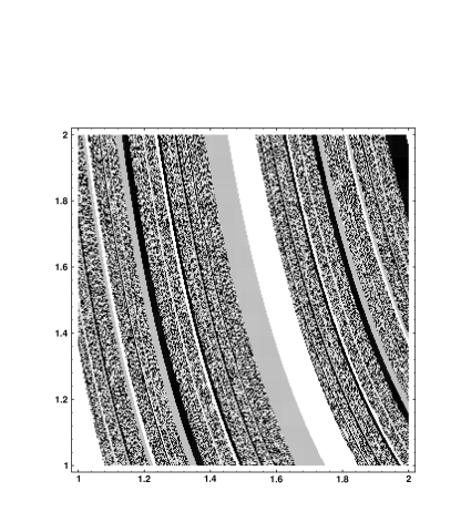
FIG. 16.: Basin boundaries in the $(u,v)$ plane for the full dynamics.

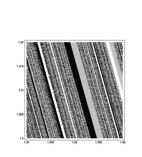
FIG. 17.: A portion of Fig. 16 magnified 50 times.

FIG. 18.: Calculating the uncertainty exponent for Fig. 17.

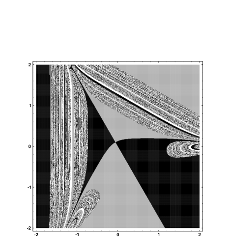
FIG. 19.: The outcome basins in the anisotropy plane.

REFERENCES

- [1] E. M. Lifshitz and I. M. Khalatnikov, Sov. Phys. Uspekhi 6, 495 (1963).
- [2] I. M. Khalatnikov and E. M. Lifshitz, Phys. Rev. Lett. 24, 76 (1970); V. A. Belinskii, I. M. Khalatnikov and E. M. Lifshitz, Adv. Phys. 19, 525 (1970).
- [3] B. K. Berger, in General Relativity and Gravitation, proceedings of GR14, gr-qc/9512003 (1995).
- [4] T. Dittrich & R. Graham, in Information Dynamics, eds. H. Atmanspacher & H. Scheingraber, (Plenum Press, NY, 1991).
- [5] Deterministic chaos in general relativity eds. D. Hobill, A. Burd and A. Coley, (Plenum Press, New York, 1994).
- [6] J. D. Barrow & F. Tipler, Phys. Rep. 56, 372 (1979).
- [7] C. W. Misner, Phys. Rev. Lett. 22, 1071, (1969).
- [8] J. D. Barrow, Phys. Rev. Lett. 46, 963 (1981); Phys. Rep. 85, 1 (1982).
- [9] D. F. Chernoff and J. D. Barrow, Phys. Rev. Lett. 50, 134 (1983).
- [10] S. E. Rugh, Cand. Scient. Thesis, The Niels Bohr Institute, (1990).
- [11] G. Francisco and G. E. A. Matsas, Gen. Rel. Grav. 20, 1047 (1988).
- [12] J. Pullin, Talk given at VII Simposio Latinoamericano de Relatividad y Gravitacion, (1990).
- [13] B. K. Berger, Gen. Rel. Grav. 23, 1385 (1991).
- [14] D. Hobill, D. Bernstein, D. Simkins and M. Welge, Class. Quant. Grav., 8, 1155 (1991).
- [15] C. P. Dettmann, N. E. Frankel and N. J. Cornish, Phys. Rev. D50, R618 (1994); Fractals, 3, 161 (1995).
- [16] N. J. Cornish and J. J. Levin, Phys. Rev. D53, 3022 (1996).
- [17] N. J. Cornish and J. J. Levin, Phys. Rev. Lett. to appear (1997), gr-qc/9605029.
- [18] B. B. Mandelbrot, Nature of Fractal Geometry, (Freeman, San Francisco, 1982).
- [19] D. N. Page, Class. Quant. Grav. 1, 417 (1984).
- [20] M. Widom, D. Bensimon, L. P. Kadanoff and S. J. Shenker, J. Stat. Phys. 32, 443 (1983); L. P. Kadanoff and C. Tang, Proc. Natl. Acad. Sci. USA 81, 443 (1984).
- [21] D. Auerbach, P. Cvitanović, J. P. Eckmann, G. Gunaratne and I. Procaccia, Phys. Rev. Lett. 58, 2387 (1987).
- [22] A. Latifi, M. Musette and R. Conte, Phys. Lett. A194, 83 (1994), G. Contopoulos, B. Grammaticos and A. Ramani, J. Phys. A27, 5357 (1994).
- [23] C. W. Misner, K. S. Thorne and J. A. Wheeler, Gravitation, (W. H. Freeman and Company, New York, 1973).
- [24] D. Mayer, Phys. Lett. A121, 390 (1987).
- [25] A. B. Burd, N. Buric and R. K. Tavakol, Class. Quant. Grav. 8, 123 (1991).
- [26] B. K. Berger, Phys. Rev. D47, 3222 (1993).
- [27] R. Cushman and J. Sniatycki, Rep. Math. Phys. 36, 75 (1995).
- [28] O. I. Bogoyavlenskii & S. P. Novikov, Sov. Phys. JETP, 37, 747 (1973).
- [29] E. Ott, Chaos in dynamical systems, (Cambridge University Press, Cambridge, 1993).
- [30] E. Ott, W. D. Withers and J. A. Yorke, J. Stat. Phys. 36, 687 (1984).
- [31] S. W. McDonald, C. Grebogi, E. Ott and J. A. Yorke, Physica D 17, 125 (1985); C. Grebogi, E. Kostelich, E. Ott and J. A. Yorke, in Dynamical systems ed. J. C. Alexander (Springer-Verlag, Berlin, 1988).
- [32] We thank Carl Dettmann for pointing this out to us.
- [33] see eg. M. Schröder Fractals, Chaos, Power Laws: Minutes from an Infinite Paradise, (W. H. Freeman and Company, New York, 1991).
- [34] The connection to the rational Farey tree was noted by S. E. Rugh and can be found in his article in Ref.[5].
- [35] R. M. Wald, General Relativity, (The University of Chicago Press, Chicago, 1984).
- [36] L. S. Young, Ergod. Th. Dynam. Syst. 2, 109 (1982); A. Fathi, Commun. Math. Phys. 126, 249 (1989).
- [37] H. Kantz and P. Grassberger, Physica D 17, 75 (1985); T. Bohr and D. Rand, Physica D 25, 387 (1987); G. H. Hsu, E. Ott and C. Grebogi, Phys. Lett. A127, 199 (1988). Z. Kovacs and L. Wiesenfeld, Phys. Rev. E51, 5476 (1995)
- [38] J. L. Kaplan and J. A. Yorke, in Functional differential equations and approximations of fixed points eds. H. O. Peitgen and H. O. Walter, (Springer, Berlin, 1979).
- [39] C. Grebogi, E. Ott, J. A. Yorke, Phys. Rev. A. 37, 1711 (1988).
- [40] D. M. Chitre, University of Maryland Ph.D. thesis (1972).
- [41] S. Bleher, C. Grebogi, E. Ott and R. Brown, Phys. Rev. A. 38, 930 (1988).
- [42] T. D. Creighton and D. W. Hobill, pg. 433 in Ref.[5].
- [43] H. Fujisaka, Prog. Theor. Phys. 70, 1264 (1983).
- [44] H. E. Nusse and J. Yorke, Physica D 36, 137 (1989).
- [45] J. D. Farmer, E. Ott and J. A. Yorke, Physica D 7, 153 (1983).
- [46] G. Montani, Class. Quant. Grav. 12, 2505, (1995).