Echoing and scaling in Einstein-Yang-Mills critical collapse

Abstract

We confirm recent numerical results of echoing and mass scaling in the gravitational collapse of a spherical Yang-Mills field by constructing the critical solution and its perturbations as an eigenvalue problem. Because the field equations are not scale-invariant, the Yang-Mills critical solution is asymptotically, rather than exactly, self-similar, but the methods for dealing with discrete self-similarity developed for the real scalar field can be generalized. We find an echoing period $\Delta=0.73784\pm 0.00002$ and critical exponent for the black hole mass $\gamma=0.1964\pm 0.0007$.

04.25.Dm, 04.20.Dw, 04.40.Nr, 04.70.Bw, 64.60.Ht

I Introduction

Recently, Choptuik, Chmaj and Bizoń [1] have studied the gravitational collapse of an $SU(2)$ Yang-Mills field restricted to spherical symmetry. Near the boundary in initial data space between data which form black holes and data which do not (“critical collapse”) they found two regions with qualitatively different behavior. In “region I” they found a mass gap, with the minimum black hole mass equal to the mass of the Bartnik-McKinnon solution, while in “region II” they found the mass scaling and echoing which are by now familiar from critical collapse in other matter models. The two kinds of behavior are reminiscent of first and second order phase transitions.

We review type I and type II behavior in section II. We shall see that each type of behavior can be understood through the presence of an intermediate attractor. The type I attractor is the well-known Bartnik-McKinnon solution, which is static and asymptotically flat. The type II attractor is self-similar and was not known before. After having derived the necessary field equations in section III, we construct it as an eigenvalue problem in section IV of this paper. In section V we construct its linear perturbations in another eigenvalue problem and verify that only one of them is growing. This allows us to calculate the critical exponent governing the mass scaling semi-analytically, without numerical collapse simulations. In section VI we summarize our results, which are in good agreement with collapse simulations, discuss how the Einstein-Yang-Mills system differs from other systems in which critical collapse has previously been studied, and put the present paper into perspective.

The analytic and numerical methods of this paper are a generalization of those developed for the spherical scalar field in [2, 3]. In contrast to the scalar field system the field equations contain a length scale $e^{-1}$ (in units $c=G=1$), where $e$ is the coupling constant in the Yang-Mills-covariant derivative $D_{a}=\nabla_{a}+eA_{a}$. The presence of a scale in the field equations excludes the existence of an exactly self-similar solution. Instead we make a series ansatz for a solution which becomes self-similar asymptotically on spacetime scales much smaller than $e^{-1}$, or equivalently for curvatures much greater than $e^{2}$. The echoing period $\Delta$ is determined by the leading term of the expansion alone. For the linearized equations we also make a series ansatz, but the spectrum $\{\lambda_{i}\}$ of Lyapunov exponents is once more determined by the first term of that series alone. Moreover, to calculate the first term of the perturbation expansion one only needs to know the first term of the background expansion. Therefore the higher terms of either expansion are not required in order to calculate both the echoing period $\Delta$ and critical exponent $\gamma$ exactly, and will not be calculated here.

II Type I and type II critical phenomena

Here we summarize the findings of Choptuik, Chmaj and Bizoń [1] and explain them in dynamical systems terms. The purpose of this section is to show that critical phenomena are, in hindsight, easy to explain, to stress the mathematical similarities between type I and type II critical behavior, and to motivate the more technical calculations in the following sections.

For introductory reviews of critical collapse, see [4, 5, 6]. Very briefly, one wants to study the limit in phase space between initial data which eventually form a black hole and data which do not. Choptuik [7] pioneered the method of (numerically) evolving initial data taken from one-parameter families of initial data which cross this boundaries, families of data, in other words, which form a black hole for large values of the parameter, $p$, but not for small values. Generic families have this property. By bisection one can numerically determine the critical value $p_{*}$ of $p$ for a given family.

For the spherically symmetric massless scalar field Choptuik found that the black hole mass could be made arbitrarily small, and scaled like $M\sim(p-p_{*})^{\gamma}$, with $\gamma\simeq 0.37$ the same for all families of data. Furthermore, before forming the black hole, the time evolution from all data with $|p-p_{*}|$ sufficiently small, from all families, approached one universal solution with the strange property of being periodic in the logarithm of both $r$ and $t$, or $\phi(r,t)=\phi(e^{\Delta}r,e^{\Delta}t)$, with a period of $\Delta\simeq 3.44$. The smaller $|p-p_{*}|$, the more “echos” were visible before the black hole formed or before the fields dispersed to infinity.

For the spherically symmetric $SU(2)$ Yang-Mills field, Choptuik, Chmaj and Bizoń [1] found the same behavior, with $\Delta\simeq 0.74$ and $\gamma\simeq 0.20$ in some region of initial data space, and called it “type II behavior” because the black hole mass resembles the order parameter in a second-order phase transition. In another region of initial data space they found that as $p$ went through $p_{*}$, the black hole mass jumped to a finite value instead of showing power law behavior. Before the black hole formed, the solution approached a regular static solution of that mass, and remained there for the longer the smaller $|p-p_{*}|$ was. They named this “type I behavior”, in analogy with a first-order phase transition.

Without keeping up the sense of mystery any longer, we now explain these phenomena in dynamical systems terms [8, 9, 4] through the presence of an “intermediate attractor”, a solution which has precisely one growing perturbation. We shall introduce a compact notation which focuses on the essential similarities and dissimilarities of the two types, while hiding the details, and which will also be useful later on: by $Z$ we denote the vector of variables of some first-order form of the field equations, such that, for example, the complete field equations in spherical symmetry can be compactly written as $F(Z,Z_{,r},Z_{,t})=0$. The presentation is best begun with type I behavior.

Type I behavior is dominated by the Bartnik-McKinnon solution [10], which is static, spherically symmetric and asymptotically flat. It has exactly one unstable perturbation mode [11], which makes it an intermediate attractor in dynamical systems terms. Let $Z_{*}^{\text{(I)}}(r)$ denote this solution. As it depends only on $r$, its general linear perturbation must be of the form $\delta Z=\sum_{i=0}^{\infty}C_{i}\,e^{\lambda_{i}t}\ \delta_{i}Z(r),$ where the $C_{i}$ are free constants. There is exactly one unstable mode, that is $\Re\lambda_{1}>0$ and $\Re\lambda_{i}<0$ for $i=2,3,\dots$. Furthermore, it is known that the final state arising from initial data $Z_{0}(r,\epsilon)\equiv Z_{*}^{\text{(I)}}(r)+\epsilon\,\delta_{1}Z(r)$ is a black hole for one sign of $\epsilon$, and flat space with outgoing waves for the other. Let $p$ be the parameter of a one-parameter-family of initial data, such that for $p>p_{*}$ a black hole forms, and for $p<p_{*}$ the solution disperses. Then for $(p-p_{*})$ sufficiently small, the time evolution of data from the family enters an intermediate asymptotic regime of the form

$$Z(r,t)\simeq Z_{*}^{\text{(I)}}(r)+{\partial C_{1}^{\text{(I)}}\over\partial p}(p_{*})\ (p-p_{*})\ e^{\lambda_{1}^{\text{(I)}}t}\ \delta_{1}^{\text{(I)}}Z(r),$$ (1)

where the decaying perturbations ($i\geq 2$) can already be neglected, and where we have approximated $C_{1}=C_{1}(p)$ linearly. This solution leaves the intermediate asymptotic regime to form a black hole or disperse at a time $T$ when the amplitude of the perturbations, $\partial C_{1}/\partial p\ (p-p_{*})\ e^{\lambda_{1}T}$, has reached some small fiducial value $\epsilon$. This gives a lifetime

$$T\sim-\lambda\ln(p-p_{*})+c$$ (2)

of the meta-stable state, where $c$ depends on the one-parameter family, but where $\lambda=1/\lambda_{1}^{\text{(I)}}$ is universal. This was in fact observed by Choptuik, Chmaj and Bizon, and used to estimate $\lambda_{1}^{\text{(I)}}$, in good agreement with perturbation theory.

The intermediate attractor in regime II is self-similar instead of static. It is in fact discretely self-similar, but that is not an essential detail, and for clarity of comparison with regime I we pretend in the introduction, and only here, that it is continuously self-similar. We also disregard the fact that the self-similarity is only asymptotic on small scales. In suitable coordinates $Z_{*}^{\text{(II)}}$ then depends only on $r/t$ instead of only on $r$. Its general linear perturbation must be of the form $\delta Z=\sum_{i=0}^{\infty}C_{i}\,t^{\lambda_{i}}\ \delta_{i}Z(r).$ Once more there is exactly one growing mode. (This is required for the explanation we are about to give to work, and we will demonstrate it explicitly in section IV.) The intermediate asymptotic regime for type II behavior is

$$Z(r,t)\simeq Z_{*}^{\text{(II)}}(r/t)+{\partial C_{1}^{\text{(II)}}\over\partial p}(p_{*})\ (p-p_{*})\ t^{\lambda_{1}^{\text{(II)}}}\ \delta_{1}^{\text{(II)}}Z(r/t).$$ (3)

One now argues from scale-invariance [8, 9, 12, 3] that the black-hole mass $M$ is proportional to $T$, and obtains for the black hole mass

$$\ln M=\gamma\ln(p-p_{*})+c,$$ (4)

where $\gamma=-1/\lambda_{1}^{\text{(II)}}$ is universal, and $c$ is a family-dependent constant.

If the scale-invariance is only asymptotic, as it is for scalar electrodynamics or Einstein-Yang-Mills, the scaling argument to calculate the black hole mass goes through unchanged [13]. If the critical solution is discretely self-similar, as for the scalar field or the model considered here, with an echoing period of $\Delta$ in the logarithm of the length and time scales, a periodic “wiggle” [3] or “fine structure” [14] is superimposed on the mass scaling law, which becomes

$$\ln M=\gamma\ln(p-p_{*})+c+\Psi[\ln(p-p_{*})+c/\gamma],$$ (5)

where $\Psi$ is a universal periodic function with period $\Delta/(2\gamma)$. (Note that the same family-dependent constant $c$ appears a second time in the argument of $\Psi$.) The form of the critical solution and its perturbations is also more complicated, and will be discussed in section IV.A and V.A respectively.

III Field equations and scaling variables

In this section we introduce coordinates and field variables for the spherically symmetric Einstein-Yang-Mills system that are adapted to type II behavior, where scale-invariance plays a crucial role. In the following we consider only type II behavior, and no longer write the index (II). We adopt the conventions and notation of [1], which include making both the Yang-Mills field and the coordinates $r$ and $t$ dimensionless by absorbing suitable factors of $G$, $c$ and $e$ into them.

The spherically symmetric spacetime metric is written as

$$ds^{2}\equiv-\alpha^{2}\,dt^{2}+a^{2}\,dr^{2}+r^{2}\left(d\vartheta^{2}+\sin^{2}\vartheta\,d\varphi^{2}\right),$$ (6)

where $a$ and $\alpha$ depend only on $r$ and $t$, and the Yang-Mills field strength is given in terms of a single potential $W(r,t)$ as

$$F\equiv dW\wedge(\tau_{1}\,d\vartheta+\tau_{2}\,\sin\vartheta\,d\varphi)-(1-W^{2})\tau_{3}d\vartheta\wedge\sin\vartheta\,d\varphi,$$ (7)

where $\tau_{i}$ are the Pauli matrices. In order to write the field equations in first order form, we define

$$\Phi\equiv W_{,r},\qquad\Pi\equiv{a\over\alpha}W_{,t}.$$ (8)

The complete field equations, reduced to spherical symmetry, are

$$r\Phi_{,t}= r\left({\alpha\over a}\Pi\right)_{,r},$$ (9)

$$r\Pi_{,t}= r\left({\alpha\over a}\Phi\right)_{,r}+a\alpha r^{-1}W(1-W^{2}),$$ (10)

$$r{a_{,r}\over a}= {1\over 2}(1-a^{2})+\Phi^{2}+\Pi^{2}+{1\over 2}a^{2}r^{-2}(1-W^{2})^{2},$$ (11)

$$r{\alpha_{,r}\over\alpha}= {1\over 2}(a^{2}-1)+\Phi^{2}+\Pi^{2}-{1\over 2}a^{2}r^{-2}(1-W^{2})^{2},$$ (12)

$$r{a_{,t}\over\alpha}= 2\Pi\Phi.$$ (13)

These equations are the Yang-Mills equation, and three of the four algebraically independent components of the Einstein equations. The fourth component is obtained by combining derivatives of the other three, and is therefore redundant.

In order to construct a discretely self-similar solutions, we follow [2, 3] in defining new coordinates

$$\tau\equiv\ln(-t),\qquad\zeta\equiv\ln\left(-{r\over t}\right)-\xi_{0}(\tau),$$ (14)

where $\xi_{0}$ is a periodic function to be determined, with period $\Delta$. (This definition differs slightly from [3] in that $t$ and $r$ are dimensionless, and that $t$ is negative.) The resulting spacetime metric is

$$ds^{2}=e^{2\tau}\left\{-\alpha^{2}\,d\tau^{2}+e^{2(\zeta+\xi_{0})}\left[a^{2}\left(d\zeta+(1+\xi_{0}^{\prime})\,d\tau\right)^{2}+d\vartheta^{2}+\sin^{2}\vartheta\,d\varphi^{2}\right]\right\},$$ (15)

where $a$ and $\alpha$ are now functions of $\zeta$ and $\tau$, and where $\xi_{0}\equiv\xi_{0}(\tau)$ and $\xi_{0}^{\prime}\equiv d\xi_{0}/d\tau$. As discussed in [3], discrete self-similarity is equivalent to $a$ and $\alpha$ being periodic in $\tau$. In the field equations we make the replacements

$$r{\partial\over\partial r}={\partial\over\partial\zeta},\qquad r{\partial\over\partial t}=e^{\zeta+\xi_{0}(\tau)}\left[-{\partial\over\partial\tau}+(1+\xi_{0}^{\prime}(\tau)){\partial\over\partial\zeta}\right],\qquad r=e^{\tau+\zeta+\xi_{0}(\tau)}$$ (16)

to transform to the new coordinates.

We shall be looking for a solution in which $a$ and $\alpha$ are periodic. What does this mean for the matter variables $\Phi$, $\Pi$ and $W$? The Einstein equations suggest that $\Phi$ and $\Pi$ should be periodic too, but $W$ cannot be periodic because of the explicit presence of the factors $e^{\tau}$ in the equations. Nor can we simply absorb such a factor into the definition of $W$ to make it periodic. This means that the equations have no nontrivial self-similar (periodic) solutions. The physical reason is the presence of the length scale $e^{-1}$ in the problem, which is only hidden by the dimensionless variables. Following a suggestion by Matt Choptuik [15], we define a new scalar field $S$ by

$$W\equiv 1-rS.$$ (17)

With this definition, the two potential terms arising in the field equations,

$$r^{-1}W(1-W^{2})=(1-rS)(2-rS)S,\qquad r^{-2}(1-W^{2})^{2}=(2-rS)^{2}S^{2},$$ (18)

split into the sum of a term which no longer contains $r$ explicitly, plus terms containing positive powers of $r$, which become negligible on small spacetime scales (as $r\to 0$ or $\tau\to-\infty$). Two further definitions, namely $\Pi_{\pm}\equiv\Pi\pm\Phi$ and $g\equiv{a/\alpha}$, will be useful because $g$ alone determines the ingoing and outgoing null geodesics, and $\Pi_{+}$ and $\Pi_{-}$ are the components of the matter field propagating along them.

In the following, we use the coordinates $\zeta$ and $\tau$, and the fields $Z\equiv\{a,g,\Pi_{+},\Pi_{-},S\}$. In these variables, the complete field equations, including the definitions of $\Pi_{+}$ and $\Pi_{-}$ in terms of $S$, are

$$\Pi_{\pm,\zeta}= {\mp e^{\zeta+\xi_{0}}g\Pi_{\pm,\tau}+C\Pi_{\pm}\mp a^{2}(1-e^{\tau+\zeta+\xi_{0}}S)(2-e^{\tau+\zeta+\xi_{0}}S)S\over 1\mp(1+\xi_{0}^{\prime})e^{\zeta+\xi_{0}}g},$$ (19)

$$a_{,\zeta}= {a\over 2}\left(C+\Pi_{+}^{2}+\Pi_{-}^{2}\right),$$ (20)

$$g_{,\zeta}= Cg,$$ (21)

$$S_{,\zeta}= -S-{1\over 2}\left(\Pi_{+}-\Pi_{-}\right),$$ (22)

$$0= a_{,\tau}+e^{-(\zeta+\xi_{0})}g^{-1}{a\over 2}\left(\Pi_{+}^{2}-\Pi_{-}^{2}\right)-(1+\xi_{0}^{\prime}){a\over 2}\left(C+\Pi_{+}^{2}+\Pi_{-}^{2}\right),$$ (23)

$$0= S_{,\tau}-e^{-(\zeta+\xi_{0})}g^{-1}{1\over 2}\left(\Pi_{+}+\Pi_{-}\right)+(1+\xi_{0}^{\prime})\left[S+{1\over 2}\left(\Pi_{+}-\Pi_{-}\right)\right],$$ (24)

where

$$C\equiv 1-a^{2}+a^{2}(2-e^{\tau+\zeta+\xi_{0}}S)^{2}S^{2}.$$ (25)

As suggested by the way we have written the equations, the first five can be treated as evolution equations in $\zeta$, with periodic boundary conditions in $\tau$, and the last two as constraints which are propagated by the evolution equations. Note that now only positive powers of $e^{\tau}$ appear explicitly, so that in the limit $\tau\to-\infty$ we are left with a set of nontrivial, scale-invariant equations for $Z$. The terms multiplied by $e^{\tau}$ are “irrelevant” in the language of renormalisation group theory [16].

The equations are invariant under $W\to-W$, and the potential for $W$ has the two minima $W=\pm 1$. In (17) we have assumed that $W\to 1$ asymptotically. A solution tending to $W=-1$ can be trivially obtained from one tending to $W=1$ by changing the sign of $W$, $\Phi$ and $\Pi$, while leaving $S$, $a$ and $\alpha$ unchanged. The field equations are left unchanged.

IV Background solution

A The eigenvalue problem

In this section we construct the solution $Z^{\text{(II)}}_{*}(r,t)$ which dominates type II behavior. To find a solution which is asymptotically self-similar in the limit $\tau\to-\infty$, that is on spacetime scales smaller than the intrinsic scale of the field equations, we make the ansatz

$$Z_{*}(\zeta,\tau)=\sum_{n=0}^{\infty}e^{n\tau}\,Z_{*n}(\zeta,\tau),$$ (26)

where each $Z_{*n}$ is periodic in $\tau$. $Z_{*0}$ is the solution of a nonlinear eigenvalue problem, with eigenvalue $\Delta$, and boundary conditions arising from certain regularity requirements. $Z_{*1}$ is the solution of an inhomogeneous nonlinear boundary value problem, with source terms depending on $Z_{*0}$. Similar boundary value problems completely determine all higher $Z_{*n}$ recursively.

In the following we are interested only in the equations for $Z_{*0}$, and from now on we suppress the suffix _∗0 on the components of $Z_{*0}$, denoting $\Pi_{+*0}$ simply by $\Pi_{+}$ etc. (In the compact formal notation $Z_{*0}$ we keep the suffix.) The equations for $Z_{*0}$ are derived from those for $Z$ above by setting the factor $e^{\tau}$ equal to zero at each explicit occurrence. We choose to evolve only $\Pi_{+}$, $\Pi_{-}$ and $g$ in $\zeta$, with eqns. (19) and (21), and to determine $a$ and $S$ at each new value of $\zeta$ from the constraints, eqns. (23) and (24). The final set of equations, those we have solved numerically, is, in the simplified notation,

$$\Pi_{\pm,\zeta}= {\mp e^{\zeta+\xi_{0}}g\Pi_{\pm,\tau}+\left(1-a^{2}+4a^{2}S^{2}\right)\Pi_{\pm}\mp 2a^{2}S\over 1\mp(1+\xi_{0}^{\prime})e^{\zeta+\xi_{0}}g},$$ (27)

$$g_{,\zeta}= \left(1-a^{2}+4a^{2}S^{2}\right)g,$$ (28)

$$0= a_{,\tau}+e^{-(\zeta+\xi_{0})}g^{-1}{a\over 2}\left(\Pi_{+}^{2}-\Pi_{-}^{2}\right)-(1+\xi_{0}^{\prime}){a\over 2}\left(1-a^{2}+4a^{2}S^{2}+\Pi_{+}^{2}+\Pi_{-}^{2}\right),$$ (29)

$$0= S_{,\tau}-e^{-(\zeta+\xi_{0})}g^{-1}{1\over 2}\left(\Pi_{+}+\Pi_{-}\right)+(1+\xi_{0}^{\prime})\left[S+{1\over 2}\left(\Pi_{+}-\Pi_{-}\right)\right].$$ (30)

All fields are periodic in $\tau$ with a period $\Delta$ that is to be determined as an eigenvalue. Here as in the example of the scalar field [3], the field equations are complemented by regularity conditions at the center $r=0$ (for $t<0$), and at the past self-similarity horizon (the past light cone of the point $(r=0,t=0)$, or $r\simeq-t$). One can solve these boundary conditions in terms of free parameters.

To make $r=0\Leftrightarrow\zeta=-\infty$ a regular center, we impose $a=1$ and $g=1$ there. We expand in powers of $e^{\zeta}$, and notice that $a$, $g$ and $\Pi$ are even in that expansion (because they are even in $r$ at $r=0$), while $S$ and $\Phi$ are odd. We label the orders of this expansion by a suffix in round brackets to distinguish them from the orders in the expansion (26). The expansion coefficients can be given recursively in terms of one free periodic function $S_{(1)}(\tau)$. To order $e^{3\zeta}$ they are, giving $\Pi$ and $\Phi$ instead of $\Pi_{+}$ and $\Pi_{-}$,

$$a_{(0)}(\tau)= 1,$$ (31)

$$g_{(0)}(\tau)= 1,$$ (32)

$$\Pi_{(0)}(\tau)= 0,$$ (33)

$$S_{(1)}(\tau)= {\rm free},$$ (34)

$$\Phi_{(1)}(\tau)= -2S_{(1)},$$ (35)

$$a_{(2)}(\tau)= 2S_{(1)}^{2},$$ (36)

$$g_{(2)}(\tau)= 0,$$ (37)

$$\Pi_{(2)}(\tau)= e^{\xi_{0}}\left[S_{(1)}^{\prime}-(1+\xi_{0}^{\prime})S_{(1)}\right],$$ (38)

$$S_{(3)}(\tau)= {1\over 10}\left\{e^{\xi_{0}}\left[\Pi_{(2)}^{\prime}-2(1+\xi_{0}^{\prime})\Pi_{(2)}\right]+8S_{(1)}^{3}\right\},$$ (39)

$$\Phi_{(3)}(\tau)= -4S_{(3)}.$$ (40)

These expressions are used to impose the asymptotic boundary condition at $\zeta\to-\infty$ at some small value of $\zeta$, say $\zeta=\zeta_{\text{left}}$.

We use the remaining coordinate freedom, the choice of $\xi_{0}(\tau)$, to move the self-similarity horizon to the coordinate surface $\zeta=0$ through the coordinate condition

$$\left[1-(1+\xi_{0}^{\prime})e^{\xi_{0}}g\right]_{\zeta=0}=0,$$ (41)

which means that $\zeta=0$ is null, and impose analyticity there by the condition

$$\left[-e^{\xi_{0}}g\Pi_{+,\tau}+(1-a^{2}+4a^{2}S^{2})\Pi_{+}-2a^{2}S\right]_{\zeta=0}=0.$$ (42)

(This is a regular and sufficient condition, by the same argument already used in [3].)

These two constraints can be solved recursively after expanding, this time in powers of $\zeta$. We denote the components of this expansion also by subscripts in round brackets. The two free parameters here are the periodic functions $g_{(0)}(\tau)$ and $\Pi_{-(0)}(\tau)$. From (41), one obtains the algebraic identity

$$g_{(0)}=[e^{\xi_{0}}(1+\xi_{0}^{\prime})]^{-1}.$$ (43)

To obtain the leading order coefficients of the other fields, we substitute (43) into eqns. (30), (29), and (27) (upper sign), obtain

$$S_{(0)}^{\prime}+(1+\xi_{0}^{\prime})S_{(0)}-(1+\xi_{0}^{\prime})\Pi_{-(0)}=0,$$ (44)

$$a_{(0)}^{\prime}-(1+\xi_{0}^{\prime})\left(\Pi_{-(0)}^{2}+{1\over 2}\right)a_{(0)}-(1+\xi_{0}^{\prime})\left(2S_{(0)}^{2}-{1\over 2}\right)a_{(0)}^{3}=0,$$ (45)

$$\Pi_{+(0)}^{\prime}-(1+\xi_{0}^{\prime})\left(1-a_{(0)}^{2}+4a_{(0)}^{2}S_{(0)}^{2}\right)\Pi_{+(0)}+(1+\xi_{0}^{\prime})2a_{(0)}^{2}S_{(0)}=0,$$ (46)

and consider these as linear ODEs for $S_{(0)}$, $(a_{(0)})^{-2}$, and $\Pi_{+(0)}$ respectively.

As in the scalar field case, we make the assumption that the metric variables $a$ and $g$ contain only even frequencies in $\tau$, and the matter variables $\Pi_{+}$, $\Pi_{-}$ and $S$ only odd frequencies. This is compatible with the equations for $Z_{*0}$, but not with the equations for the general $Z$. If this symmetry did not hold, the right-hand side of eqn. (24) would contain even terms in $\tau$, and among them generically a term constant in $\tau$. Then $S$ would not be periodic in $\tau$, but would have a term linear in $\tau$, and through the Einstein equations this would be in contradiction to the periodicity of $\alpha$ and $g$, and hence the self-similarity of $Z_{*0}$.

The equivalent of the field $S$ here is the scalar field $\phi$ in the scalar field model, and for a massive or self-interacting $\phi$ a similar argument holds. The equations for a massless $\phi$, however, do not contain $\phi$ itself but only its derivatives $\Pi_{\pm}$. Therefore a linear dependence of $\phi$ on $\tau$ would not clash with spacetime self-similarity. Such solutions exist, and have been investigated in [17], but surprisingly the critical solution for the massless field is not of this kind, and the massless and massive (or self-interacting) scalar field are therefore in the same universality class.

B Numerical construction

Our numerical method has been described in detail elsewhere [3]. By decomposing all fields in Fourier components with respect to $\tau$, the PDEs in $\tau$ and $\zeta$ go over into a (large) system of ODEs in the variable $\zeta$ for the Fourier components. ODEs in $\tau$ alone, in the boundary conditions and the constraints, go over into algebraic equations which can be solved in closed form. $\Delta$ now appears as a parameter in the Fourier transformation of the $\tau$-derivatives.

A solution of the field equations and boundary conditions exists only for isolated values of $\Delta$, and we have found precisely one. The convergence radius of our relaxation algorithm is smaller than for the scalar field, probably because of the shorter period $\Delta$, and instead of an ad-hoc initial guess we had to use collapse data kindly provided by Matt Choptuik [15] to obtain a good enough starting value for the relaxation algorithm.

We find good agreement of $Z_{*0}$ with the $Z$ of a critical collapse simulation for $-3.00<\tau<-2.22$ [15], which is not very surprising as we started our numerical search with these data, but nevertheless confirms that the ansatz (26) for $Z_{*}$ is consistent and converges for small enough $\tau$, with $Z_{*0}$ the dominant term.

To obtain error bars on the solution, we have checked convergence with the numerical parameters, $\zeta_{\text{left}}$, the number $N$ of Fourier components and the grid spacing $\Delta\zeta$, by varying one of them at a time.

Fig. 1 demonstrates quartic convergence with $\exp\zeta_{\text{left}}$, as expected from our expansion to order $O(\exp 3\zeta_{\text{left}})$. This convergence breaks down at very small values of $\exp\zeta_{\text{left}}$, due to the fact that all fields become very small.

Fig. 2 demonstrates quadratic convergence with grid spacing in $\zeta$, as expected from centered differencing of the $\zeta$-derivatives. This convergence breaks down at very small values of $\Delta\zeta$, probably because grid points get very close to the regular singular point $\zeta=0$.

Convergence with $N$ is rapid: The difference between results for $N=64$ and $N=128$ is already of order $10^{-6}$. $N=64$ is surprisingly small, given that it means only 16 odd Fourier components each to represent $\Pi_{+}(\tau)$ and $\Pi_{-}(\tau)$ and 16 even components for $g(\tau)$ and 15 for $\xi_{0}(\tau)$. (The component $\cos(4\pi/\Delta)$ of $\xi_{0}(\tau)$ is taken to be zero to fix the translation invariance in $\tau$ of the equations for $Z_{*0}$.)

For the production run we have chosen $\zeta_{\text{left}}=-6.4$, $\Delta\zeta=(1/80)$ (that is, 513 grid points) and $N=128$. The solution $Z_{*0}(\zeta,\tau)$ has an estimated maximal error of $\pm 2.3\cdot 10^{-4}$ and root-mean-square error of $\pm 3.6\cdot 10^{-5}$, in the region $-6.4\leq\zeta\leq 0$. We obtain $\Delta=0.73784\pm 0.00002$. All three error estimates are dominated by the error from finite differencing in $\zeta$, with the estimated error from expanding around $\zeta=-\infty$ somewhat smaller, and the error from using a finite number of Fourier components in $\tau$ much smaller.

V Linear perturbations and critical exponent

A The eigenvalue problem

In this section we construct the one linear perturbation of the critical solution that grows with decreasing spacetime scale, as $\tau\to-\infty$, with the purpose of calculating the critical exponent for the black hole mass in critical collapse.

The evolution equations for a linear perturbation $\delta Z$ of the background critical solution $Z_{*}$ are of the general form

$$\delta Z_{,\zeta}=A\ \delta Z_{,\tau}+(B+e^{\tau}C+e^{2\tau}D)\ \delta Z.$$ (47)

The constraints are of the same general form, but with the left-hand side equal to zero, and the following considerations apply equally to them as well. The perturbation equations differ from those for the scalar field model through the explicit appearance of $e^{\tau}$ in the equations, and the fact that the coefficients $A$, $B$, $C$ and $D$ are not periodic in $\tau$ because the background solution $Z_{*}$ is not. Like $Z_{*}$, the coefficients $A$, $B$, $C$ and $D$ derived from it admit an expansion of the form

$$A=\sum_{n=0}^{\infty}e^{n\tau}A_{n}(\zeta,\tau),$$ (48)

where the $A_{n}$ are periodic. In this expansion, the leading terms $A_{0}$, $B_{0}$, etc. depend only on the leading term $Z_{*0}$ of the background expansion.

As for the scalar field model, we make the ansatz [3]

$$\delta Z(\zeta,\tau)=\sum_{i=1}^{\infty}C_{i}\ e^{\lambda_{i}\tau}\,\delta_{i}Z(\zeta,\tau),$$ (49)

where the $C_{i}$ are free coefficients, and the $\lambda_{i}$ are a discrete set of complex numbers, which are determined as eigenvalues of a new, linear boundary value problem. Clearly the $\delta_{i}Z$ obey the equations

$$\delta_{i}Z_{,\zeta}=A\ \delta_{i}Z_{,\tau}+(B+\lambda_{i}A+e^{\tau}C+e^{2\tau}D)\ \delta_{i}Z.$$ (50)

In the massless scalar field model, the $\delta_{i}Z$ could be assumed to be periodic in $\tau$. In the presence of a scale, this is no longer possible, and we have to expand each $\delta_{i}Z$ once more as [13]

$$\delta_{i}Z(\zeta,\tau)=\sum_{n=0}^{\infty}e^{n\tau}\ \delta_{in}Z(\zeta,\tau),$$ (51)

where only the individual coefficients $\delta_{in}Z$ are periodic. This expansion is exactly analogous to (26). The $\delta_{in}Z$ obey a coupled set of equations which can be derived from (50) in a straightforward bookkeeping exercise, after inserting the expansion (48). These equations are complemented by regularity conditions at $\zeta=-\infty$ and $\zeta=0$. The equations for the $\delta_{i0}Z$ are simply

$$\delta_{i0}Z_{,\zeta}=A_{0}\ \delta_{i0}Z_{,\tau}+(B_{0}+\lambda_{i}A_{0})\ \delta_{i0}Z.$$ (52)

This equation, together with the boundary conditions, already determines the spectrum $\{\lambda_{i}\}$. The other $\delta_{in}Z$ obey inhomogeneous equations and can be determined recursively, but here we are interested only in the spectrum. This also means that we only need the leading term $Z_{*0}$ of the background expansion.

Writing down the field equations (52) for the $\delta_{i0}Z$ is straightforward. As we have seen, one simply linearizes eqns. (27-30) for $Z_{*0}$, and then makes the replacement $\delta Z_{*0,\tau}\to\delta_{i0}Z_{,\tau}+\lambda_{i}\,\delta_{i0}Z_{,\tau}$, which follows from the definition (49). Writing $a$ for $a_{*0}$, etc., and $\delta a$ for $\delta_{i0}a$, etc., to keep the notation simple, we obtain

$$\delta\Pi_{\pm,\zeta}= \left[1\mp(1+\xi_{0}^{\prime})e^{\zeta+\xi_{0}}\right]^{-1}\Bigl{\{}\mp e^{\zeta+\xi_{0}}\left[\Pi_{\pm,\tau}\ \delta g+g(\delta\Pi_{\pm,\tau}+\lambda_{i}\ \delta\Pi_{\pm})\right]+(1-a^{2}+4a^{2}S^{2})\ \delta\Pi_{\pm}$$ (54)

$$+2a(4S^{2}-1)\Pi_{\pm}\ \delta a+8a^{2}S\Pi_{\pm}\ \delta S\mp 2a^{2}\ \delta S\mp 4aS\ \delta a\pm(1+\xi_{0}^{\prime})e^{\zeta+\xi_{0}}\Pi_{\pm,\zeta}\ \delta g\Bigr{\}},$$

$$\delta g_{,\zeta}= (1-a^{2}+4a^{2}S^{2})\ \delta g+2a(4S^{2}-1)g\ \delta a+8a^{2}Sg\ \delta S,$$ (55)

$$0= \delta a_{,\tau}+\left[\lambda_{i}+{1\over 2}e^{-(\zeta+\xi_{0})}g^{-1}(\Pi_{+}^{2}-\Pi_{-}^{2})-{1\over 2}(1+\xi_{0}^{\prime})(1-3a^{2}+12a^{2}S^{2}+\Pi_{+}^{2}+\Pi_{-}^{2})\right]\delta a$$ (58)

$$+\Biggl{\{}e^{-(\zeta+\xi_{0})}\left[-{1\over 2}(\Pi_{+}^{2}-\Pi_{-}^{2})g^{-2}a\ \delta g+g^{-1}a(\Pi_{+}\ \delta\Pi_{+}-\Pi_{-}\ \delta\Pi_{-})\right]$$

$$-(1+\xi_{0}^{\prime})\left[4a^{3}S\ \delta S+a(\Pi_{+}\ \delta\Pi_{+}+\Pi_{-}\ \delta\Pi_{-})\right]\Biggr{\}},$$

$$0= \delta S_{,\tau}+(\lambda_{i}+1+\xi_{0}^{\prime})\ \delta S+{1\over 2}\left\{e^{-(\zeta+\xi_{0})}\left[g^{-2}(\Pi_{+}+\Pi_{-})\ \delta g-g^{-1}(\delta\Pi_{+}+\delta\Pi_{-})\right]+(1+\xi_{0}^{\prime})(\delta\Pi_{+}-\delta\Pi_{-})\right\}.$$ (59)

Similarly, we obtain the expansion around $\zeta=-\infty$ of the $\delta_{i0}Z$ by linearizing eqns. (31-40) and then making the same replacement, at each order in $e^{\zeta}$. The nonvanishing expansion coefficients to $O(e^{3\zeta})$ are:

$$\delta S_{(1)}(\tau)= {\rm free},$$ (60)

$$\delta\Phi_{(1)}(\tau)= -2\ \delta S_{(1)},$$ (61)

$$\delta a_{(2)}(\tau)= 4S_{(1)}\ \delta S_{(1)},$$ (62)

$$\delta\Pi_{(2)}(\tau)= e^{\xi_{0}}\left[\delta S_{(1)}^{\prime}+(\lambda-1-\xi_{0}^{\prime})\ \delta S_{(1)}\right],$$ (63)

$$\delta S_{(3)}(\tau)= {1\over 10}\left\{e^{\xi_{0}}\left[\delta\Pi_{(2)}^{\prime}+(\lambda-2-2\xi_{0}^{\prime})\ \delta\Pi_{(2)}\delta\right]+24S_{(1)}^{2}\ \delta S_{(1)}\right\},$$ (64)

$$\delta\Phi_{(3)}(\tau)= -4\ \delta S_{(3)}.$$ (65)

As the linearized regularity condition at $\zeta=0$ we impose the vanishing of the numerator of (54, upper sign). There is no linearized equivalent of the coordinate condition (41), as we have fixed the coordinate system already when the background was calculated. (In other words, $\zeta=0$ is null only on the background spacetime, not on the perturbed spacetime.) The one boundary condition at $\zeta=0$ can be solved recursively in terms of two free periodic functions $\delta g_{(0)}(\tau)$ and $\delta\Pi_{-(0)}(\tau)$, from

$$\delta S_{(0)}^{\prime}+(\lambda_{i}+1+\xi_{0}^{\prime})\ \delta S_{(0)}+(1+\xi_{0}^{\prime})\left[-\delta\Pi_{-(0)}+{1\over 2}g^{-1}\left(\Pi_{+(0)}+\Pi_{-(0)}\right)\ \delta g_{(0)}\right]=0,$$ (66)

$$\delta a_{(0)}^{\prime}+\left[\lambda_{i}+(1+\xi_{0}^{\prime})\left(-\Pi_{-(0)}^{2}-{1\over 2}+{3\over 2}a_{(0)}^{2}-6a_{(0)}^{2}S_{(0)}^{2}\right)\right]\ \delta a_{(0)}$$ (67)

$$-(1+\xi_{0}^{\prime})\left[{1\over 2}g_{(0)}^{-1}a_{(0)}\left(\Pi_{+(0)}^{2}-\Pi_{-(0)}^{2}\right)\ \delta g_{(0)}+4a_{(0)}^{3}S_{(0)}\ \delta S_{(0)}+2a_{(0)}\Pi_{-(0)}\ \delta\Pi_{-(0)}\right]=0,$$ (68)

$$\delta\Pi_{+(0)}^{\prime}+\left[\lambda_{i}-(1+\xi_{0}^{\prime})\left(1-a_{(0)}^{2}+4a_{(0)}^{2}S_{(0)}^{2}\right)\right]\ \delta\Pi_{+(0)}+g_{(0)}^{-1}\left[\Pi_{+(0)}^{\prime}-(1+\xi_{0}^{\prime})\Pi_{+(1)}\right]\ \delta g_{(0)}$$ (69)

$$+(1+\xi_{0}^{\prime})\left\{2a_{(0)}\left[\left(1-4S_{(0)}^{2}\right)\Pi_{+(0)}+2S_{(0)}\right]\ \delta a_{(0)}+2a_{(0)}^{2}\left[1-4S_{(0)}\Pi_{+(0)}\right]\ \delta S_{(0)}\right\}=0.$$ (70)

The suffix $(0)$ denotes the leading term in an expression in powers of $\zeta$ around $\zeta=0$. We still need to calculate the background term $\left(\Pi_{+,\zeta}\right)_{(0)}=\Pi_{+(1)}$ in eqn. (70). To do this, we expand eqns. (27, lower sign), (22) and (24) to $O(\zeta)$, evaluate the resulting algebraic expressions

$$g_{(1)}= C_{(0)}g_{(0)},\quad\text{where}\quad C_{(0)}\equiv 1-a_{(0)}^{2}+4a_{(0)}^{2}S_{(0)}^{2},$$ (71)

$$\Pi_{-(1)}= {1\over 2}\left[(1+\xi_{0}^{\prime})^{-1}\Pi_{-(0)}^{\prime}+C_{0}\Pi_{-0}+2a_{(0)}^{2}S_{(0)}\right],$$ (72)

$$S_{(1)}= -S_{(0)}-{1\over 2}\left(\Pi_{+(0)}-\Pi_{-(0)}\right),$$ (73)

$$a_{(1)}= {a_{(0)}\over 2}\left(C_{(0)}+\Pi_{+(0)}^{2}+\Pi_{-(0)}^{2}\right),$$ (74)

(alternatively, we could have obtained $S_{(1)}$ and $a_{(1)}$ from expanding the constraints (58) and (59)), and finally solve the linear ODE

$$\Pi_{+(1)}^{\prime} -(1+\xi_{0}^{\prime})(1+2C_{(0)})\ \Pi_{+(1)}+(1+C_{(0)})\Pi_{+(0)}^{\prime}$$ (76)

$$+(1+\xi_{0}^{\prime})\left\{2a_{(0)}\left[\left(1-4S_{(0)}^{2}\right)\Pi_{+(0)}+2S_{(0)}\right]\ a_{(1)}+2a_{(0)}^{2}\left[1-4S_{(0)}\Pi_{+(0)}\right]\ S_{(1)}\right\}=0$$

for $\Pi_{+(1)}$.

Linear perturbations which have the same $\tau$-symmetry as the background $Z_{*0}$ ($S$ and $\Pi_{\pm}$ odd frequencies, $a$ and $g$ even frequencies) decouple from those with the opposite symmetry. We call them even and odd perturbations respectively, and can treat them separately in the numerical calculation of the spectrum $\{\lambda_{i}\}$.

B Numerical construction

Our numerical method is the same as in [3]. We evolve a basis of all linear perturbations compatible with the constraints at either one of the boundaries to a matching point, and look for zeros of the determinant of that basis as a function of $\lambda$. A zero indicates the existence of a perturbation consistent with both sets of boundary conditions for that value of $\lambda$. We have implemented this algorithm for both real and complex $\lambda$. We have checked our results, for real $\lambda$ and even perturbations, with a relaxation algorithm, which is partially independent numerically, and in which $\lambda$ figures as an additional variable, which is balanced by fixing the perturbations as an additional boundary condition. The determinant in question is in fact a holomorphic function of $\lambda$ (because the field equations are real), and this can be used to find its zeros and poles efficiently.

We expect certain zeros and poles in the $\lambda$-plane from the following considerations. $Z_{*0}$ is scale-invariant, and therefore invariant under the infinitesimal transformation

$$Z_{*0}(r,t)\to Z_{*0}[(1+\epsilon)r,(1+\epsilon)t]\simeq Z_{*0}(\zeta,\tau+\epsilon)\simeq Z_{*0}(\zeta,\tau)+\epsilon Z_{*0,\tau}.$$ (77)

This corresponds to a gauge linear perturbation mode with $\lambda_{i}=0$ and $\delta_{i}Z=Z_{*0,\tau}$. $Z_{*0}$ is also invariant under time translation,

$$Z_{*0}(r,t)\to Z_{*0}(r,t+\epsilon)\simeq Z_{*0}(\zeta,\tau)+\epsilon\ e^{-\tau}\left[(1+\xi_{0}^{\prime})Z_{*0,\zeta}-Z_{*0,\tau}\right],$$ (78)

corresponding to a gauge mode with $\lambda_{i}=-1$. Both gauge modes are even according to our classification.

The ODEs, eqns. (66, 68, 70), are all of the form $f^{\prime}+gf+h=0$, where $f$ stands for $\delta S_{(0)}$, $\delta a_{(0)}$ and $\delta\Pi_{+(0)}$ respectively. In all three equations $g$ depends only on the background solution and is even, while $h$ is linear in the perturbations, and has the same $\tau$-symmetry as $f$. It can be shown [3] that this type of equation has no solution when the average value (in $\tau$) of the coefficient $g$ vanishes. As $g$ in each case is of the form $\lambda+(\text{background fields})$, this corresponds to a simple pole in the $\lambda$-plane. These poles are not just due to the breakdown of a particular numerical method but indicate that for these values of $\lambda$ no perturbations exist which obey the boundary condition at $\zeta=0$. The poles arise only when the inhomogeneous term $h$, and in consequence the unknown $f$, have a nonvanishing average, that is when they are even.

Calculating the average value of $g$ for each of the three equations, we find that they vanish for $\lambda=-1$, $\lambda=-1-A$ and $\lambda=-A$ respectively, where $A$ is the average value of $2(1+\xi_{0}^{\prime})\Pi_{-(0)}^{2}$, with numerical value $A\simeq 0.1726$. (We have used the fact that

$$(\ln a_{(0)})^{\prime}=(1+\xi_{0}^{\prime})\left[\Pi_{-(0)}^{2}+{1\over 2}+\left(2S_{(0)}^{2}-{1\over 2}\right)a_{(0)}^{2}\right]$$ (79)

has vanishing average value, as it is the derivative of a periodic function, to simplify the averages.) In summary, for even perturbations we expect zeros at $\lambda=0$ and $\lambda=-1$ (gauge modes), one more zero on the negative real line (the unstable mode) and a pole at $\lambda\simeq-1.17$. For odd perturbations we expect poles at $\lambda=-1$ and $\lambda\simeq-0.17$.

The numerical calculation of the perturbation determinant as a function of $\lambda$ largely confirms the predictions: For even perturbations, on the negative real line we find a zero at $\lambda_{1}\simeq-5.0$, corresponding to the expected physical unstable mode, with a critical exponent of $-1/\lambda_{1}\simeq 0.2$, as found in collapse simulations. We also find the expected zero at $\lambda_{2}=0$. We have verified that the corresponding $\delta_{i}Z\propto Z_{*0,\tau}$ to high precision. We find the expected pole at $\lambda\simeq-1.17$, but accompanied by a zero very close by. For odd perturbations, on the negative real line we find the expected pole at $\lambda\simeq-0.17$.

At $\lambda=-1$, for both even and odd perturbations, we do not find the expected zero and pole respectively because of a numerical problem which is discussed in the appendix. It does not affect our calculation of the perturbation determinant for values of $\lambda$ not close to $-1$. The unstable mode at $\lambda\simeq-5.0$ and gauge mode at $\lambda=0$ are clear enough, and we can use their convergence properties to obtain an estimate of the numerical error.

Table 1 gives the values of $\lambda$ for the unstable mode $\lambda_{1}$ and the scale change gauge mode $\lambda_{2}$ as a function of the step size $\Delta\zeta$. The deviation of the numerical value of $\lambda_{2}$ from zero serves as one estimate of numerical error. It is larger than the other estimate, from the convergence of $\lambda_{1}$, and we therefore adopt it as our definitive error estimate for $\lambda_{1}$. We obtain $\lambda_{1}=-5.091\pm 0.017$, from which we obtain for the critical exponent $\gamma=-1/\lambda_{1}=0.1964\pm 0.0007$.

VI Conclusions

We have obtained the asymptotic form of the type II critical solution of Einstein-Yang-Mills collapse, its echoing period, and the critical exponent for the black hole mass, in a calculation similar to the one we made for the massless scalar field [2, 3]. The major new feature is the presence of the length scale in the Einstein-Yang-Mills field equations. In consequence, the critical solution and its linear perturbations are no longer self-similar, but become so only asymptotically on spacetime scales much smaller than the length scale of the field equations (on the order of the Bartnik-McKinnon [10] mass). Here we have only calculated the leading term in the asymptotic expansions for the critical solution and its perturbations, but this is sufficient to calculate both the echoing period $\Delta$ and critical exponent $\gamma$ exactly. We find $\Delta=0.73784\pm 0.00002$ and $\gamma=0.1964\pm 0.0007$, while Choptuik, Chmaj and Bizoń [1] find $\Delta\simeq 0.74$ and $\gamma\simeq 0.20$ in collapse simulations. Data files of the background and unstable mode from the production run are available through the WWW address http://www.aei-potsdam.mpg.de/$\sim$gundlach.

In the formalism we have developed here to deal with the presence of a length scale in the equations, the leading perturbation term, $\sum C_{i}e^{\lambda_{i}\tau}\delta_{i0}Z$, obeys field equations which are the linearized version of the equations for the leading background term, $Z_{*0}$. Both sets of equations consistently describe a new physical system which is scale-invariant, and which is obtained from the original, scale-dependent, model in the limit where all fields vary on spacetime scales much smaller than the intrinsic scale of the field equations. In the language of renormalisation group theory, these equations are the short-scale fixed point of a renormalisation group transformation acting on the original field equations. In the case of a massless or self-interacting scalar field this fixed point is the massless scalar field [9]. For scalar electrodynamics, the fixed point is the massless complex scalar without electromagnetism [13]. In both cases the field equations at the fixed point can naturally be associated with the Lagrangian of a simpler physical system, and the renormalisation group acts naturally on the dimensionful coupling constant. While the latter is still true for the spherically symmetric Einstein-Yang-Mills system, the equations (27-30) are not the spherical reduction of some set of covariant field equations. The reduction to spherical symmetry does not commute with the action of the renormalisation group.

We believe that in the present paper we have developed the most general formalism that will be be required to deal with critical collapse restricted to spherical symmetry, in allowing for self-similarity and the presence of a length scale. The generalization to more than one scale is trivial: the various scales can be written as a single scale times dimensionless numbers. The general formalism has already given rise to a bit of new physics: the calculation of critical exponents not only for the black hole mass but also its charge in critical collapse of scalar electrodynamics [13].

The example of Einstein-Yang-Mills collapse shows that one does not need scale-invariance of the field equations to have type II critical phenomena with the famous relation $M\sim(p-p_{*})^{\gamma}$. Rather they can be found in some region of initial data space for any system. For astrophysical matter, these initial data are simply not realized in astrophysical collapse.

Most remaining questions in critical phenomena go beyond the restriction to spherical symmetry. Do the spherical critical solutions found so far act also as critical solutions for generic, non-spherical, initial data? What is the angular momentum of the black hole formed from data with angular momentum in the limit where the black hole mass is fine-tuned to zero? Are there qualitatively new phenomena away from spherical symmetry?

A Numerical problems at $\lambda\simeq-1$

Calculating the determinant of even perturbations as a function of $\lambda$, we do not find the expected zero but a pole at $\lambda=-1$, with an alternating series of poles and zeros accumulating towards $-1$ from below. There are no further poles or zeros immediately above. The positions of the poles are the same in the real and complex algorithms, but depend on the values of the numerical parameters $N$ and $\delta\zeta$. A qualitatively similar picture arises for odd perturbations. These features can be explained as a numerical artifact as follows.

We have checked explicitly that the gauge mode (78) obeys the constraint (58). When we try to reconstruct $\delta a$ of this mode from the constraint, however, the numerical result blows up at small $\zeta$. To understand this, consider the equation $\delta a^{\prime}+g\ \delta a+h=0$, with $g$ and $h$ defined by eqn. (58). The Fourier algorithm that we use to solve this for $\delta a$ at each $\zeta$ needs to divide the average of $h$ by the average of $g$. As $\zeta\to-\infty$, the average of $g$ over $\tau$ as a function of $\lambda$ and $\zeta$ is $\lambda+1+O(e^{2\zeta})$, where the last term is positive. As $\lambda\to-1$ from below, this goes through zero at some small value of $\zeta$. In the exact perturbation mode (78), the average value of $h$ vanishes at the same rate with $\zeta$ as that of $g$, but with small numerical errors this cancellation fails, and small numerical errors are magnified. In the calculation of the perturbation determinant this results in the observed, essentially random behavior for $\lambda\lesssim-1$. For $\lambda>-1$ the problem does not arise, as then the average value of $g$ does not vanish for any $\zeta$.

We have not found a simple way of fixing this problem, as our algorithm relies in an essential way on reconstructing $S$ and $a$ and $\delta S$ and $\delta a$ from the constraints at each $\zeta$. It does not affect numerical results however unless where the average values of both the coefficients $g$ and $h$ are very small, that is for $\lambda\lesssim-1$. (If only the average value of $g$ is small, the resulting blowup in the perturbations is physical, as in the other poles we have discussed.) Calculating the perturbation determinant is not goal in itself, but only a means of finding the spectrum of linear perturbations. With the present method we can say with confidence that there is a zero at $\lambda\simeq-5.0$, and no other zeros for negative real $\lambda$, apart from the two gauge modes. We could in principle be missing a zero (physical growing mode) at $\lambda\lesssim-1$, where the code is unreliable, and have to rely on evidence from collapse simulations that there is only one unstable mode.

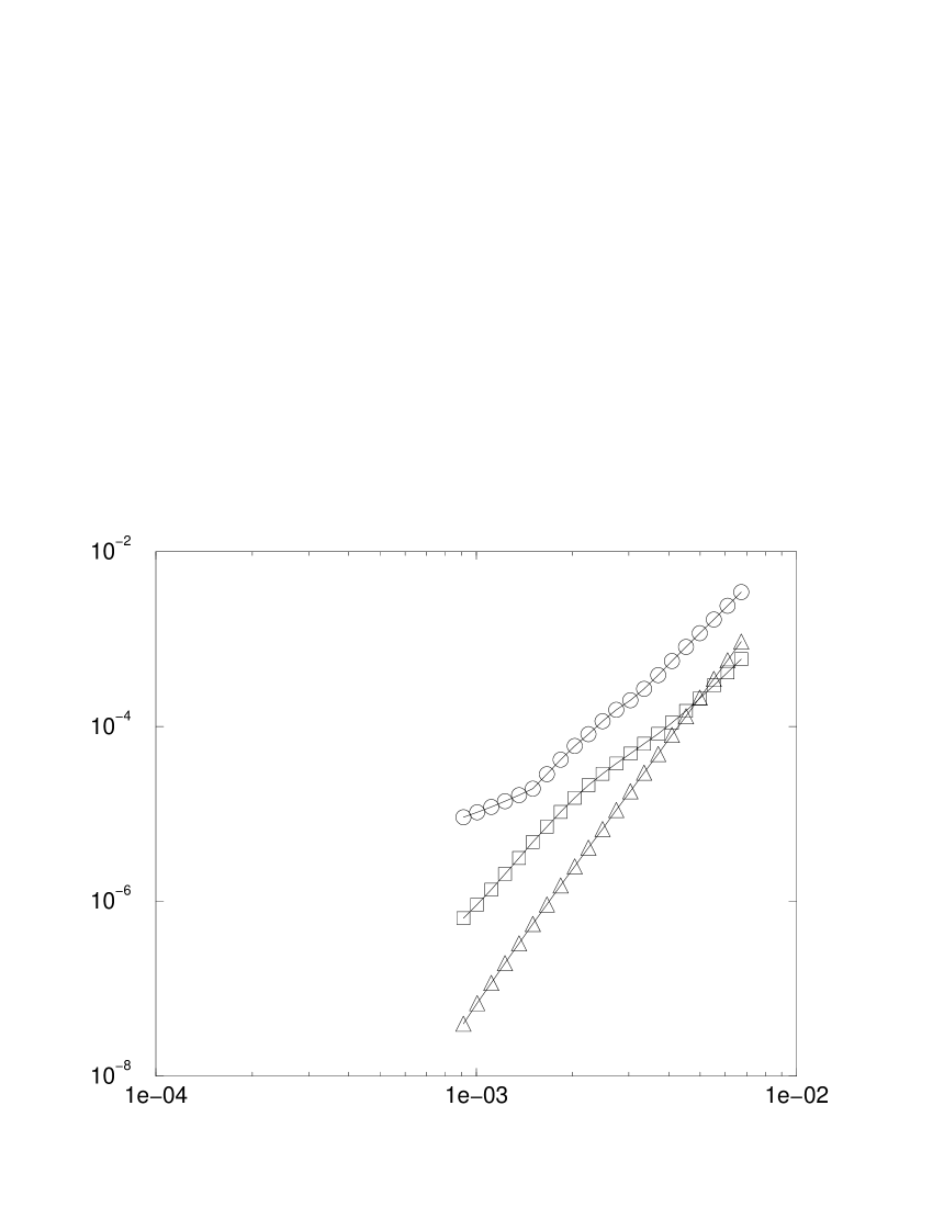
FIG. 1.: Quartic convergence of $Z_{*0}$ with $\exp\zeta_{\text{left}}$. Assuming that the error is $E\simeq A\exp 4\,\zeta_{\text{left}}$, the difference between two numerical solutions obtained with $\zeta_{\text{left}}$ and $\zeta_{\text{left}}+\Delta\zeta_{\text{left}}$ is $E^{\prime}\simeq 4A\,\Delta\zeta_{\text{left}}\,\exp 4\,\zeta_{\text{left}}$. Therefore we plot here $E^{\prime}/(4\Delta\zeta_{\text{left}})\simeq E$, against $\exp\zeta_{\text{left}}$. Circles denote the maximal error, over all gridpoints and Fourier components, squares the root mean square error, and triangles the error in $\Delta$. $N=64$ and $\Delta\zeta=0.1$. The production value $\zeta_{\text{left}}=-6.4$ corresponds to the fifth point from the left.

FIG. 2.: Quadratic convergence of $Z_{*0}$ with $\Delta\zeta$. As a measure of the error at $\Delta\zeta$, we compare with $\Delta\zeta/2$. Circles denote the maximal error, over all gridpoints and Fourier components, squares the root mean square error, and triangles the error in $\Delta$. $N=64$ and $\zeta_{\text{left}}=-6.4$. The production value $\Delta\zeta=(1/80)$ corresponds to the second point from the left.

TABLE I.: Convergence of $\lambda$ with step size in $\zeta$. $\lambda_{1}$ is the Lyapunov exponent of the one growing mode. Its negative inverse is the critical exponent $\gamma$. $\lambda_{2}$ is the exponent of the scale change ($\tau$-translation) gauge mode. It must be zero and serves as a check on the numerical error. Note that the numerical grid (and number of steps) is the same for the background as for the perturbations in each case. The range of $\zeta$ is $-6.4\leq\zeta\leq 0$ in each case.

Number of steps	$\lambda_{1}$	$\lambda_{2}$
32	-5.1318584162589	0.13720816860828
64	-5.0828194924873	-1.4932102080912E-02
128	-5.0891816495598	-1.1519697001693E-02
256	-5.0910562847918	4.7061190684163E-03
512	-5.0913625725286	1.6758611037677E-02

REFERENCES

- [1] M. W. Choptuik, T. Chmaj and P. Bizon, Phys. Rev. Lett. 77, 424 (1996).
- [2] C. Gundlach, Phys. Rev. Lett. 75, 3214 (1995).
- [3] C. Gundlach, Understanding critical collapse of a scalar field, gr-qc/9604019, to be published in Phys. Rev. D.
- [4] P. Bizoń, How to make a tiny black hole, gr-qc/9606060.
- [5] J. Horne, Matters of Gravity, 7, 14 (1996), gr-qc/9602001.
- [6] C. Gundlach, Critical phenomena in gravitational collapse, gr-qc/9606023.
- [7] M. W. Choptuik, Phys. Rev. Lett. 70, 9 (1993).
- [8] T. Koike , T. Hara, and S. Adachi, Phys. Rev. Lett. 74, 5170 (1995).
- [9] T. Hara, T. Koike , and S. Adachi, Renormalisation group and critical behavior in gravitational collapse, gr-qc/9607010.
- [10] R. Bartnik and J. McKinnon, Phys. Rev. Lett. 61, 141 (1988).
- [11] Z.-H. Zhou and N. Straumann, Phys. Lett. B 243, 33 (1990). See also G. Lavrelashvili and D. Maison, Phys. Lett. B 343, 214 (1995).
- [12] E. W. Hirschmann and D. M. Eardley, Phys. Rev. D 52, 5850 (1995).
- [13] C. Gundlach and J. M. Martin-Garcia, Charge scaling and universality in critical collapse, gr-qc/9606072, to be published in Phys. Rev. D.
- [14] S. Hod and T. Piran, Fine-structure of Choptuik’s mass-scaling relation, gr-qc/9606087.
- [15] M. W. Choptuik, private communication.
- [16] J. Bricmont and A. Kupiainen, Renormalizing Partial Differential Equations, chao-dyn/9411015.
- [17] P. Brady, Phys. Rev. D 51 4168, (1995).